Planckian superconductor

The Bardeen-Cooper-Schrieffer mechanism of conventional superconductivity Bardeen et al. (1957) requires two species of fermions coupled by an attractive two-body interaction. Altland and Simons (2010) The mean-field analysis of such a model results in the gapped quasiparticle excitation spectrum below the critical temperature. Meanwhile, the absence of long-living quasiparticles in high-temperature superconducting materials above the critical temperature is an immutable characteristic of the so-called strange metal state. Senthil (2008); Keimer et al. (2015) In contrast to the quasiparticle nature of superconductors, strange metals exhibit a power-law behavior in the spectral function, Varma et al. (1989) similarly to quantum critical systems. Sachdev (2011) A lack of quasiparticles manifests itself in fast equilibration at low temperature on a timescale set by the Planckian relaxation time $t_{\mathrm{P}}=\hbar/\left(2\pi k_{\mathrm{B}}T\right)$. Zaanen (2004); Sachdev (2011) The same timescale appears as an upper bound on quantum chaos setting the maximal rate of information scrambling. Maldacena et al. (2016) It is usually formulated Maldacena et al. (2016); Shenker and Stanford (2015); Roberts and Swingle (2016) in terms of the out-of-time ordered correlator Larkin and Ovchinnikov (1969) (OTOC): In quantum many-body systems the OTOC grows no faster than exponentially $e^{t/t_{\mathrm{L}}}$ with the Lyapunov time $t_{\mathrm{L}}$ bounded from below as $t_{\mathrm{L}}\geq t_{\mathrm{P}}$. Maldacena et al. (2016)

The widely known Sachdev-Ye-Kitaev (SYK) model, Sachdev and Ye (1993); Kitaev (2015) describing strongly interacting Majorana zero modes in $0+1$ dimensions, saturates the chaos bound $t_{\mathrm{L}}=t_{\mathrm{P}}$. Kitaev (2015); Maldacena and Stanford (2016) It does not possess an underlying quasiparticle description while being solvable in the infrared, with a spectral function that scales as a power law of frequency. These properties do not change upon replacing Majoranas with conventional fermions (complex SYK model). Sachdev (2015); Bulycheva (2017) The extensions of this model to the cSYK coupled clusters predict thermal diffusivity Davison et al. (2017) $\propto t_{\mathrm{P}}$ and reproduce the linear in temperature resistivity, Song et al. (2017) observed in strange metals. Takagi et al. (1992); Taillefer (2010) Recently, a proposed theory of a Planckian metal, Patel and Sachdev (2019) based on the destruction of a Fermi surface by the cSYK-like interactions, shows that the universal scattering time equals the Planckian time $t_{\mathrm{P}}$. The latter one characterizes the linear in temperature resistivity property Bruin et al. (2013) and was detected in cuprates, Legros et al. (2019) pnictides, Nakajima et al. (2019) and twisted bilayer graphene, Cao et al. (2019) regardless of their different microscopic nature.

The success in applying the SYK model to qualitative studies of strange metals and the minimalistic structure of the model itself fostered the effort to find a mechanism by which the superconducting state is formed out of an incoherent SYK metal. Patel et al. (2018); Esterlis and Schmalian (2019); Wang (2019); Chowdhury and Berg (2019) Driven by the same curiosity, we consider a $(0+1)$-dimensional toy model which consists of a superconducting quantum dot Kouwenhoven and Marcus (1998) coupled to the complex-valued SYK model. Sachdev (2015) At the critical coupling the pairing gap turns out to be proportional to the Planckian relaxation rate at low temperatures,

where $\eta$ is a number close to one. This theoretical finding that we refer to as a Planckian superconductor draws parallels to the phenomenon of reentrant superconductivity Maple et al. (1972); Simons et al. (2012) in Kondo superconductors Müller-Hartmann and Zittartz (1971); Riblet and Winzer (1971); Müller-Hartmann et al. (1976) and the physics of Andreev billiards. Melsen et al. (1997); Schomerus and Beenakker (1999); Lodder and Nazarov (1998); Adagideli and Beenakker (2002); Vavilov and Larkin (2003)

We start with a superconducting Hamiltonian $H_{\rm SC}$ that contains $2M$ modes described by the Richardson Hamiltonian Richardson (1963); von Delft et al. (1996); Matveev and Larkin (1997) without single-particle energies coupled to the SYK model $H_{\rm SYK}$ with $N$ fermions through a random tunneling term $H_{\rm tun}$,

The couplings $t^{\sigma}_{ij}$ and $J_{ij;kl}$ are assumed to be independent Gaussian random variables with finite variances $\overline{{t^{\sigma}}^{*}_{ij}t^{\sigma^{\prime}}_{ij}}=t^{2}\delta_{\sigma\sigma^{\prime}}$, $\overline{|J_{ij;kl}|^{2}}=J^{2}$ ($J_{ij;kl}=-J_{ji;kl}=-J_{ij;lk}=J^{*}_{kl;ij}$), and zero means.

The interaction terms in the Hamiltonian (2) are decoupled within the Hubbard-Stratonovich transformations, Altland and Simons (2010); Sachdev (2015) so that in the large $M,N$ limit the self-consistent saddle-point equations are app (a)

where $\omega_{n}=\pi T(2n+1)$ are Matsubara frequencies and $p=M/N$ controls the ratio between the “sites” Banerjee and Altman (2017); Chen et al. (2017); Jian and Yao (2017) in the superconductor/SYK sector. The self-energy of the SYK fermions appears in the equations (6,7) as $\Sigma_{c}(\tau)$, while $G_{c}(\tau)$ denotes the corresponding Green’s function $-N^{-1}\sum_{i=1}^{N}\left\langle\mathrm{T}_{\tau}c_{i}(\tau)\bar{c}_{i}(0)\right\rangle$. The Green’s functions of the $\uparrow$,$\downarrow$ fermions in the superconductor $G_{\sigma}(\tau)=-M^{-1}\sum_{i=1}^{M}\left\langle\mathrm{T}_{\tau}\psi_{i\sigma}(\tau)\bar{\psi}_{i\sigma}(0)\right\rangle$ enter the equation (8) as a half trace of the Gor’kov’s function Gor’kov (1958) $G_{+}(\tau)=\tfrac{1}{2}(G_{\uparrow}+G_{\downarrow})(\tau)$. Finally, relation (9) is a modified gap equation, Altland and Simons (2010) which accounts for the amount of the SYK impurity in the superconductor through $G_{c}(\tau)$ under the assumption of frequency independent pairing $\Delta$. The chemical potential $\mu$ can be accounted in the equations (6-9) by the shift $|\Delta|^{2}\to|\Delta|^{2}+\mu^{2}$. Below, we set $\mu=0$.

In the normal phase ($\Delta=0$) the equations (6-8) can be written as

ensuring a convenient self-energy translation $\Sigma\equiv\Sigma_{c}-2\sqrt{p}\,t^{2}G_{+}$. If $p\ll 1/2$ ($2M\ll N$), the bare SYK Green’s function $G_{\rm SYK}(\mathrm{i}\omega_{n})=-\mathrm{i}\pi^{1/4}\mathrm{sgn}\left(\omega_{n}\right)/\sqrt{|J\omega_{n}|}$ solves the equations (10,11) in the infrared $\omega_{n}\ll J$. In this regime, the Green’s function of the $\psi$ fermions $G_{+}(\mathrm{i}\omega_{n})$ scales as $\sqrt{\omega_{n}}$ for $\omega_{n}/J\ll p^{-1/3}(t/J)^{4/3}$. In the equal sites case $2M=N$, which corresponds to $p=1/2$, the bare SYK Green’s function survives for $\left(t/J\right)^{4/3}\ll\omega_{n}/J\ll 1$. Another solution appears at $p=1/2$ if one supposes $\omega_{n}\ll\left\{t^{2}\left|G_{c}\right|,\left|\Sigma\right|\right\}$. Then the equation (11) shortens to

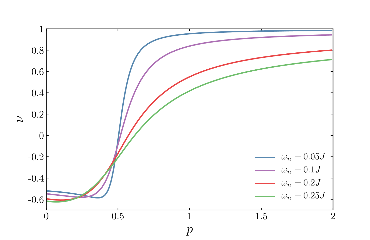
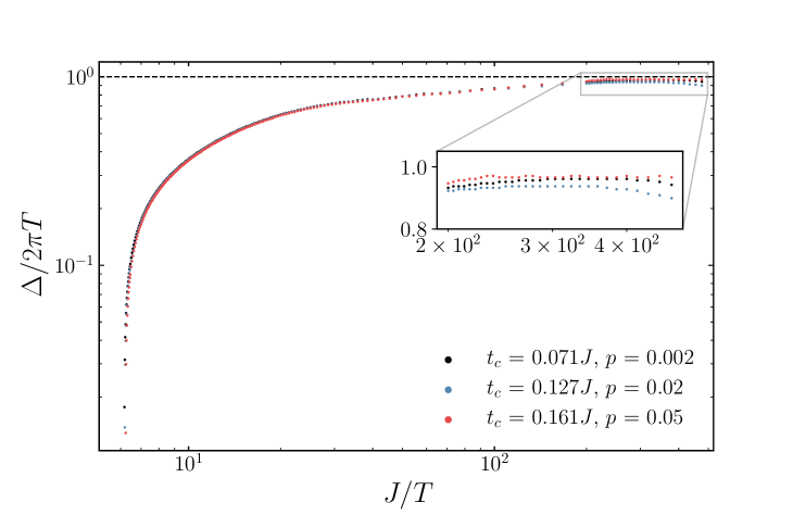
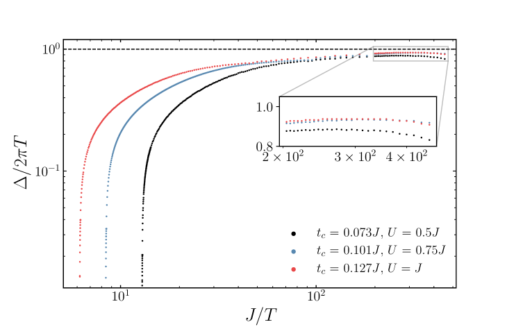
The Green’s function that satisfies the equations (10,12) is $G_{c}(\mathrm{i}\omega)\propto-\mathrm{i}\,\mathrm{sgn}(\omega)/\left(J^{2}t^{2}|\omega_{n}|\right)^{\!-1/5}$ for the frequencies $\left(t/J\right)^{3}\ll\omega_{n}/J\ll\left(t/J\right)^{4/3}$, that are achievable in the weak tunneling limit $t\ll J$. Note that the frequency window strictly depends on the coupling $t$. For $p\gg 1/2$, the Green’s function of the $c$ fermions in the low-frequency limit is $G_{c}(\mathrm{i}\omega_{n})\propto-\mathrm{i}\omega_{n}$, Jian and Yao (2017) which leads to the density of states $-\pi^{-1}\mathrm{Im}G_{c}(\mathrm{i}\omega_{n}\to\omega+\mathrm{i}0^{+})\simeq 0$ vanishing in the SYK sector. Therefore, at large $p$, the normal phase is given by the free fermions in the $\psi$–dot, whose Green’s function is $G_{+}(\mathrm{i}\omega_{n})=-\mathrm{i}/\omega_{n}$. To follow the frequency scaling of the Green’s function $G_{c}(\mathrm{i}\omega_{n})$ while changing $p$, we introduce the logarithmic derivative $\nu=\partial\ln G_{c}/\partial\ln\omega_{n}$ plotted in Figure 1 at low temperatures. Summarizing, the normal phase in the infrared limit is described by the inverse Green’s function of the SYK model at small $p$, whereas it crosses over to free fermions for large $p$ values.

The gap equation (9) at $\Delta=0$ makes a boundary in between the normal phase and the superconducting one by setting the critical temperature $T_{c}$ as a function of the coupling rate $t$. Let us notice that the SYK model (4) does not have a spin degree of freedom after disorder averaging. app (a) Thus, it may be thought of as spin polarized. It suppresses superconductivity similar to magnetic impurities: Increase of the coupling to the SYK subsystem decreases the critical temperature. De Gennes (1966) There exists a critical coupling $t_{c}$,

such as to abolish superconductivity at zero temperature. The constraint (13) follows from the gap equation (9) when $\Delta,T=0$.

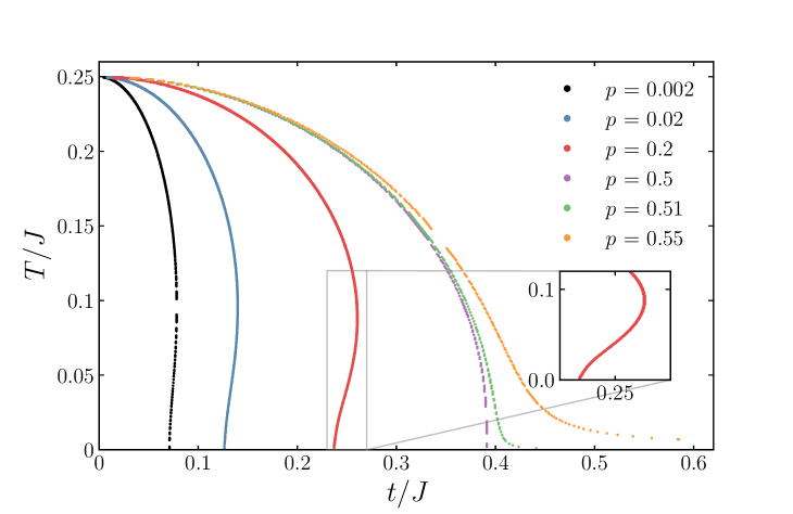
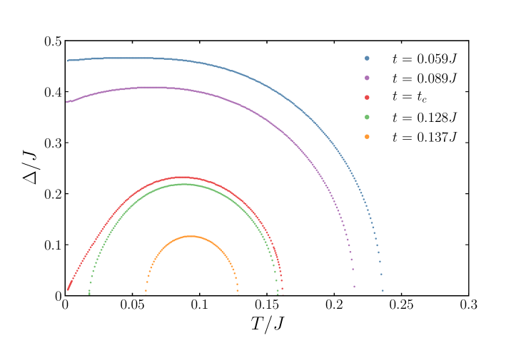
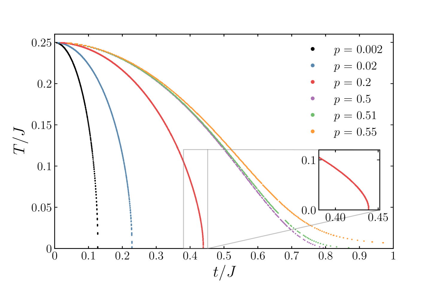
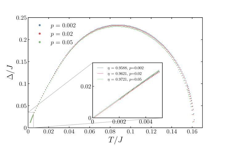
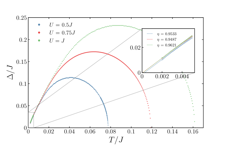
There are three competing phases contributing to the denominator of the self-consistency relation (9): SYK non-Fermi liquid, free fermions, and superconducting condensate $\Delta$. If there are enough of the SYK fermions ($N>2M$), $\Delta$ interplays with the non-Fermi liquid at zero temperature. The latter one falls off with an increase in temperature, making room for the superconducting phase beyond the critical coupling, which results in the growth of the critical temperature. Indeed, Figure 2 (left) shows the bend of the critical temperature in the vicinity of the critical coupling. com (a) This phenomenon resembles the reentrant superconductivity Maple et al. (1972); Simons et al. (2012) in superconductors with Kondo impurities. Müller-Hartmann and Zittartz (1971); Riblet and Winzer (1971); Müller-Hartmann et al. (1976) The pairing gap goes down at low temperatures with an increase in coupling as in Figure 2 (right). Achieving the critical coupling when $\Delta$ vanishes at zero temperature leads to the appearance of the lower critical temperature. In contrast, the reentrant superconducting regime is absent for $N<2M$, since the normal phase behaves as the conventional Fermi liquid at low temperatures and large $p$, as was noticed earlier. In Figure 2 (left), we show com (a) that $p=1/2$ ($N=2M$) separates the regions with one or two critical temperatures. Similarly, consideration of the random free fermion model $\sum_{ij}J_{ij}c^{\dagger}_{i}c_{j}$ instead of the SYK model does not give the reentrance effect. In this case, the self-energy equation (6) changes to $\Sigma_{c}(\mathrm{i}\omega_{n})=J^{2}G_{c}(\mathrm{i}\omega_{n})+2\sqrt{p}\,t^{2}G_{+}(\mathrm{i}\omega_{n})$. The results for the critical temperature are presented in Figure 3. It is still possible to suppress the superconductivity at zero temperature providing sufficient impurities, but there is only a single critical temperature as the normal phase is always set by the free fermions. com (b)

From Figure 2 (right), one notices the pairing gap at the critical coupling is $\propto T$ at low temperatures. We numerically examine com (a) $\Delta$ in the reentrant phase $p<1/2$ for several values of $p$ and $U$ (see Figure 4). The gap saturates $2\pi T$ almost irrespective of parameters of the problem. Unit recovery brings us to the above-mentioned relation (1) so that the gap is set by the inverse Planckian time $1/t_{\mathrm{P}}$ multiplied by $\hbar$.

This observation seems to be reminiscent of quite a peculiar feature of an Andreev billiard: Beenakker (2005) In a clean chaotic cavity proximate to a superconductor, the induced gap equals $\hbar/t_{\mathrm{E}}=\hbar/\!\left(t_{\mathrm{L}}\ln\frac{p_{\mathrm{F}}l}{\hbar}\right)$,Lodder and Nazarov (1998); Adagideli and Beenakker (2002); Vavilov and Larkin (2003) where $t_{\mathrm{E}}$ is the Ehrenfest time (the typical timescale of quantum dynamics), $t_{\mathrm{L}}$ is the Lyapunov time, $p_{\mathrm{F}}$ is the Fermi momentum, and $l$ is the characteristic cavity length. The effect is predicted in the regime of the Ehrenfest time far exceeds $\tau$ the typical lifetime of an electron/hole excitation in the cavity. Oppositely, if $t_{\mathrm{E}}\ll\tau$, the gap behaves as $\hbar/\tau$, where $\tau$ does not depend on the Planck constant. Melsen et al. (1997); Schomerus and Beenakker (1999) In the SYK model the Lyapunov time coincides with the Planckian relaxation time $t_{\mathrm{L}}=\hbar/\left(2\pi k_{\mathrm{B}}T\right)=t_{\mathrm{P}}$, Kitaev (2015); Maldacena and Stanford (2016) although those are different physical quantities. com (d) However, the Ehrenfest time is $t_{\mathrm{L}}\ln N\gg\hbar/(2\pi k_{\mathrm{B}}T)$, which differs from $t_{\mathrm{P}}$ predicted in the pairing gap (1) by $\ln N$.

To estimate the gap behavior at the critical coupling we consider the equations (6-8) at finite $\Delta$,

whereas the self-energy equation (10) stays unchanged. The right-hand side of the equation (14) tends to unity for $p\ll 1/2$. Thus it is sufficient to substitute the SYK Green’s function in the gap equation (9) in this regime.

As we look for a low-temperature correction to zero $\Delta$ at the critical coupling, we expand the gap equation (9) in powers of $\Delta$ up to the second order,

The SYK Green’s function diverges at low frequencies as $1/\sqrt{\omega_{n}}$ and decays as $1/\omega_{n}$ in the ultraviolet. Hence the principal contribution to the sum (15) from the high frequencies is given by the bare $\omega_{n}$ in the denominator. On the other hand, a divergent Green’s function is crucial at low frequencies. Assuming $G_{c}$ decays fast enough in comparison to $\omega_{n}$, we replace $G_{c}$ with the infrared SYK Green’s function $G_{SY\!K}(\mathrm{i}\omega_{n})=-\mathrm{i}\pi^{1/4}\mathrm{sgn}\left(\omega_{n}\right)/\sqrt{|J\omega_{n}|}$ in expression (15).

The low-temperature version of relation (15) can be written by means of the Euler-Maclaurin formula, Abramowitz and Stegun (1964)

where we expand up to $T^{2}$ keeping in mind that $\Delta\propto T$ at the critical coupling. com (e) Finally, one notices two terms in the top row of the equation (16) that match the critical coupling condition (13). Therefore, we obtain com (f)

Although this estimate gives $\eta\approx 1.22$ that exceeds the found numerical value $\eta\approx 0.96$ for the pairing gap $\Delta\approx\eta\,\hbar/t_{\mathrm{P}}$, the derived low-temperature gap behavior (17) is independent of the problem parameters as in Figure 4.

Conclusion.— In this manuscript, we considered the superconducting proximity effect for the Sachdev-Ye-Kitaev model. We have shown, that the superconducting dot coupled to the complex SYK model possesses reentrant superconductivity. At the critical coupling, which gives rise to the occurrence of a lower critical temperature, the pairing gap disappears at $T=0$ and grows linearly with an increase in temperature. The linear–$T$ growth of the gap is given by $\hbar/t_{\mathrm{P}}$, where $t_{\mathrm{P}}=\hbar/\left(2\pi k_{\mathrm{B}}T\right)$ is the Planckian relaxation time. The same timescale serves as an ultimate bound on many-body quantum chaos, Maldacena et al. (2016) saturated in strongly coupled systems without quasiparticle excitations. Thereby a natural question arises whether the pairing gap is an appropriate physical observable for the Lyapunov spectrum Romero-Bermúdez et al. (2019) of the SYK model. Accurate studies of the OTOC in the proposed system (2) might shed light on that. On its own, $\Delta\approx\eta\,\hbar/t_{\mathrm{P}}$ may be used to characterize the cSYK quantum dots. Chen et al. (2018); Danshita et al. (2017) However, this requires consideration of a more realistic setup such as a superconducting lead attached to the particular realization of the complex SYK model.

References

- Bardeen et al. (1957) J. Bardeen, L. N. Cooper, and J. R. Schrieffer, Phys. Rev. 108, 1175 (1957).
- Altland and Simons (2010) A. Altland and B. D. Simons, Condensed Matter Field Theory, 2nd ed. (Cambridge University Press, 2010).
- Senthil (2008) T. Senthil, Phys. Rev. B 78, 035103 (2008).
- Keimer et al. (2015) B. Keimer, S. A. Kivelson, M. R. Norman, S. Uchida, and J. Zaanen, Nature 518, 179–186 (2015).
- Varma et al. (1989) C. M. Varma, P. B. Littlewood, S. Schmitt-Rink, E. Abrahams, and A. E. Ruckenstein, Phys. Rev. Lett. 63, 1996 (1989).
- Sachdev (2011) S. Sachdev, Quantum Phase Transitions, 2nd ed. (Cambridge University Press, 2011).
- Zaanen (2004) J. Zaanen, Nature 430, 512–513 (2004).
- Maldacena et al. (2016) J. Maldacena, S. H. Shenker, and D. Stanford, Journal of High Energy Physics 2016, 106 (2016).
- Shenker and Stanford (2015) S. H. Shenker and D. Stanford, Journal of High Energy Physics 2015, 132 (2015).
- Roberts and Swingle (2016) D. A. Roberts and B. Swingle, Phys. Rev. Lett. 117, 091602 (2016).
- Larkin and Ovchinnikov (1969) A. I. Larkin and Y. N. Ovchinnikov, Sov. Phys. JETP 28, 1200 (1969).
- Sachdev and Ye (1993) S. Sachdev and J. Ye, Phys. Rev. Lett. 70, 3339 (1993).
- Kitaev (2015) A. Kitaev, KITP Program: Entanglement in Strongly-Correlated Quantum Matter (2015).
- Maldacena and Stanford (2016) J. Maldacena and D. Stanford, Phys. Rev. D 94, 106002 (2016).
- Sachdev (2015) S. Sachdev, Phys. Rev. X 5, 041025 (2015).
- Bulycheva (2017) K. Bulycheva, Journal of High Energy Physics 2017, 69 (2017).
- Davison et al. (2017) R. A. Davison, W. Fu, A. Georges, Y. Gu, K. Jensen, and S. Sachdev, Phys. Rev. B 95, 155131 (2017).
- Song et al. (2017) X.-Y. Song, C.-M. Jian, and L. Balents, Phys. Rev. Lett. 119, 216601 (2017).
- Takagi et al. (1992) H. Takagi, B. Batlogg, H. L. Kao, J. Kwo, R. J. Cava, J. J. Krajewski, and W. F. Peck, Phys. Rev. Lett. 69, 2975 (1992).
- Taillefer (2010) L. Taillefer, Annual Review of Condensed Matter Physics 1, 51 (2010).
- Patel and Sachdev (2019) A. A. Patel and S. Sachdev, Phys. Rev. Lett. 123, 066601 (2019).
- Bruin et al. (2013) J. A. N. Bruin, H. Sakai, R. S. Perry, and A. P. Mackenzie, Science 339, 804 (2013).
- Legros et al. (2019) A. Legros, S. Benhabib, W. Tabis, F. Laliberté, M. Dion, M. Lizaire, B. Vignolle, D. Vignolles, H. Raffy, Z. Z. Li, P. Auban-Senzier, N. Doiron-Leyraud, P. Fournier, D. Colson, T. L., and C. Proust, Nature Physics 15, 142–147 (2019).
- Nakajima et al. (2019) Y. Nakajima, T. Metz, C. Eckberg, K. Kirshenbaum, A. Hughes, R. Wang, L. Wang, S. R. Saha, I.-L. Liu, N. P. Butch, D. Campbell, Y. S. Eo, D. Graf, Z. Liu, S. V. Borisenko, P. Y. Zavalij, and J. Paglione, (2019), arXiv:1902.01034 [cond-mat.str-el] .
- Cao et al. (2019) Y. Cao, D. Chowdhury, D. Rodan-Legrain, O. Rubies-Bigordà, K. Watanabe, T. Taniguchi, T. Senthil, and P. Jarillo-Herrero, (2019), arXiv:1901.03710 [cond-mat.str-el] .
- Patel et al. (2018) A. A. Patel, M. J. Lawler, and Eu.-A. Kim, Phys. Rev. Lett. 121, 187001 (2018).
- Esterlis and Schmalian (2019) I. Esterlis and J. Schmalian, Phys. Rev. B 100, 115132 (2019).
- Wang (2019) Y. Wang, (2019), arXiv:1904.07240 [cond-mat.str-el] .
- Chowdhury and Berg (2019) D. Chowdhury and E. Berg, (2019), arXiv:1908.02757 [cond-mat.str-el] .
- Kouwenhoven and Marcus (1998) L. Kouwenhoven and C. Marcus, Physics World 11, 35 (1998).
- Maple et al. (1972) M. Maple, W. Fertig, A. Mota, L. DeLong, D. Wohlleben, and R. Fitzgerald, Solid State Communications 11, 829 (1972).
- Simons et al. (2012) Y. B. Simons, O. Entin-Wohlman, Y. Oreg, and Y. Imry, Phys. Rev. B 86, 064509 (2012).
- Müller-Hartmann and Zittartz (1971) E. Müller-Hartmann and J. Zittartz, Phys. Rev. Lett. 26, 428 (1971).
- Riblet and Winzer (1971) G. Riblet and K. Winzer, Solid State Communications 9, 1663 (1971).
- Müller-Hartmann et al. (1976) E. Müller-Hartmann, B. Schuh, and J. Zittartz, Solid State Communications 19, 439 (1976).
- Melsen et al. (1997) J. A. Melsen, P. W. Brouwer, K. M. Frahm, and C. W. J. Beenakker, Physica Scripta T69, 223 (1997).
- Schomerus and Beenakker (1999) H. Schomerus and C. W. J. Beenakker, Phys. Rev. Lett. 82, 2951 (1999).
- Lodder and Nazarov (1998) A. Lodder and Yu. V. Nazarov, Phys. Rev. B 58, 5783 (1998).
- Adagideli and Beenakker (2002) İ. Adagideli and C. W. J. Beenakker, Phys. Rev. Lett. 89, 237002 (2002).
- Vavilov and Larkin (2003) M. G. Vavilov and A. I. Larkin, Phys. Rev. B 67, 115335 (2003).
- Richardson (1963) R. Richardson, Physics Letters 3, 277 (1963).
- von Delft et al. (1996) J. von Delft, A. D. Zaikin, D. S. Golubev, and W. Tichy, Phys. Rev. Lett. 77, 3189 (1996).
- Matveev and Larkin (1997) K. A. Matveev and A. I. Larkin, Phys. Rev. Lett. 78, 3749 (1997).
- app (a) See Appendix A.
- Banerjee and Altman (2017) S. Banerjee and E. Altman, Phys. Rev. B 95, 134302 (2017).
- Chen et al. (2017) X. Chen, R. Fan, Y. Chen, H. Zhai, and P. Zhang, Phys. Rev. Lett. 119, 207603 (2017).
- Jian and Yao (2017) S.-K. Jian and H. Yao, Phys. Rev. Lett. 119, 206602 (2017).
- Gor’kov (1958) L. P. Gor’kov, Sov. Phys. JETP 7, 505 (1958).
- De Gennes (1966) P. De Gennes, Superconductivity of Metals and Alloys (Benjamin, 1966).
- com (a) The full self-consistent scheme (6-9) is solved numerically with the adaptive golden ratio algorithm [Malitsky, 2019,app, b].
- com (b) Earlier it was shown that the superconducting instability in the unparticle system leads to the reentrance effect as well [Karch et al., 2016], whereas restoration of the quasiparticles makes the critical temperature a single-valued function of the pairing strenth.
- com (c) The gap decrease in Figure 4 at very low temperatures (see the enlarged segments) has a numerical origin. As Matsubara frequencies are , achieving temperatures close to zero requires a sufficient increase of the numerical grid. This leads to the accuracy reduce due to the computer memory overflow [app, b].
- Beenakker (2005) C. W. J. Beenakker, “Andreev billiards,” in Quantum Dots: a Doorway to Nanoscale Physics, edited by W. Dieter Heiss (Springer Berlin Heidelberg, Berlin, Heidelberg, 2005) pp. 131–174.
- com (d) The equilibration time and the Lyapunov time are a priori different physical quantities. Nevertheless, the fact that both quantities are subjected to the same bound raises the question of whether those two seemingly independent quantities might be related. This hypothesis has been intensively investigated in the context of the AdS/CFT correspondence, in large– vector models and spin systems (see [Couch et al., 2019] and the references therein). In systems with a small parameter (large– quantum field theories or weakly coupled field theories) where a regime of exponential growth is present in the OTOC, however, they are set by the same physics even though they are quantitatively different [Grozdanov et al., 2018,Grozdanov et al., 2019].
- Abramowitz and Stegun (1964) M. Abramowitz and I. A. Stegun, Handbook of Mathematical Functions with Formulas, Graphs, and Mathematical Tables (Dover, 1964).
- com (e) Similarly, in large– models, the primary contribution of low Matsubara frequencies to the gap equation leads to [Wu et al., 2019].
- com (f) We use .
- Romero-Bermúdez et al. (2019) A. Romero-Bermúdez, K. Schalm, and V. Scopelliti, Journal of High Energy Physics 2019, 107 (2019).
- Chen et al. (2018) A. Chen, R. Ilan, F. de Juan, D. I. Pikulin, and M. Franz, Phys. Rev. Lett. 121, 036403 (2018).
- Danshita et al. (2017) I. Danshita, M. Hanada, and M. Tezuka, Progress of Theoretical and Experimental Physics 2017, 8, 083I01 (2017).
- com (g) We compute the corresponding Green’s functions in time representation with the adapted Fast Fourier Transform each iteration.
- Malitsky (2019) Yu. Malitsky, Math. Program. (2019), doi:10.1007/s10107-019-01416-w.
- app (b) See Appendix B.
- Karch et al. (2016) A. Karch, K. Limtragool, and P. W. Phillips, Journal of High Energy Physics 2016, 175 (2016).
- Couch et al. (2019) J. Couch, S. Eccles, P. Nguyen, B. Swingle, and S. Xu, (2019), arXiv:1908.06993 [cond-mat.stat-mech] .
- Grozdanov et al. (2018) S. Grozdanov, K. Schalm, and V. Scopelliti, Phys. Rev. Lett. 120, 231601 (2018).
- Grozdanov et al. (2019) S. Grozdanov, K. Schalm, and V. Scopelliti, Phys. Rev. E 99, 012206 (2019).
- Wu et al. (2019) Y.-M. Wu, A. Abanov, Y. Wang, and A. V. Chubukov, Phys. Rev. B 99, 144512 (2019).