Planning and Control of Multi-Robot-Object Systems under Temporal Logic Tasks and Uncertain Dynamics
Abstract
We develop an algorithm for the motion and task planning of a system comprised of multiple robots and unactuated objects under tasks expressed as Linear Temporal Logic (LTL) constraints. The robots and objects evolve subject to uncertain dynamics in an obstacle-cluttered environment. The key part of the proposed solution is the intelligent construction of a coupled transition system that encodes the motion and tasks of the robots and the objects. We achieve such a construction by designing appropriate adaptive control protocols in the lower level, which guarantee the safe robot navigation/object transportation in the environment while compensating for the dynamic uncertainties. The transition system is efficiently interfaced with the temporal logic specification via a sampling-based algorithm to output a discrete path as a sequence of synchronized actions of the robots; such actions satisfy the robots’ as well as the objects’ specifications. The robots execute this discrete path by using the derived low level control protocol. Simulation results verify the proposed framework.
Index Terms:
Multi-agent systems, multi-agent-object systems, linear temporal logic, robot navigation, cooperative manipulation, object transportation, multi.I Introduction
Temporal-logic-based motion planning has gained significant amount of attention over the last decade, as it provides a fully automated correct-by-design controller synthesis approach for autonomous robots. Temporal logics, such as linear temporal logic (LTL), provide formal high-level languages that can describe planning objectives more complex than the well-studied navigation algorithms, and have been used extensively both in single- as well as in multi-robot setups (see, indicatively, [1, 2, 3, 4, 5, 6, 7, 8, 9, 10]). The task is given as a temporal logic formula, which is coupled with a discrete representation of the underlying system, abstracted from the underlying continuous dynamics, in order to derive an appropriate high-level discrete path.
There exist numerous works that consider temporal-logic-based tasks, both for single- and multi-robot systems [1, 2, 3, 5, 7, 9]. Nevertheless, the related works consider temporal logic-based motion planning for fully actuated, autonomous robotic agents. Consider, however, cases where some unactuated objects must undergo a series of processes in a workspace with autonomous robots (e.g., car factories or automated warehouses). In such cases, the robots, except for satisfying their own motion specifications, are also responsible for coordinating with each other in order to transport the objects around the workspace. When the unactuated objects’ specifications are expressed using temporal logics, then the abstraction of the robots’ behavior becomes much more complex, since it has to take into account the objects’ goals.
In addition, the spatial discretization of a multi-agent system to an abstracted higher level system necessitates the design of appropriate continuous-time controllers for the transition of the agents among the states of discrete system. Many works in the related literature, however, either assume that there exist such continuous controllers or adopt non-realistic assumptions. For instance, many works either do not take into account continuous agent dynamics or consider single or double integrators [3, 9, 1, 8, 10], which can deviate from the actual dynamics of the agents, leading thus to poor performance in real-life scenarios. Discretized abstractions, including design of the discrete state space and/or continuous-time controllers, can be found in [7, 11, 12, 13, 14] for general systems and [15, 16] for multi-agent systems. Moreover, many works adopt dimensionless point-mass agents and therefore do not consider inter-agent collision avoidance [7, 9, 10], which can be a crucial safety issue in applications involving autonomous robots.
Since we aim at incorporating the unactuated objects’ specifications in our framework, the robots have to perform (cooperative) transportation of the objects around the workspace, while avoiding collisions with obstacles. Cooperative transportation/manipulation has been extensively studied in the literature (see, for instance, [17, 18, 19, 20, 21, 22, 23, 24, 25, 26, 27]), with collision avoidance specifications being incorporated in [28, 24, 25]. Cooperative object transportation under temporal logics has also been considered in our previous work [29].
This paper proposes a novel algorithm for the motion and task planning of a multi-robot-object system, i.e., a system that consists of multiple robots and unactuated objects, subject to tasks that are expressed by LTL constraints. We consider that the robots and the objects evolve subject to continuous-time and -space dynamics that suffer from uncertainties and in an environment cluttered with obstacles. Our contribution is summarized as follows. First, we abstract the continuous dynamics of the multi-robot-object system into a finite transition system that encodes the coupled behavior of the robots and the objects in the environment. We achieve such an abstraction by developing continuous feedback-control protocols that guarantee i) the navigation of the robots and ii) the cooperative transportation of the objects by the robots in the environment. These protocols combine barrier functions and point-world transformations to guarantee collision-avoidance properties as well as adaptive-control methodologies to compensate for the dynamic uncertainties. The robot navigation and cooperative object transportation constitute robot action primitives that enable the transitions in the aforementioned transition system. Second, we compose the resulting transition system with an automaton-based representation of the underlying LTL task. Finally, we use a sampling-based procedure to search the composition of the transition system and the task’s automaton for the derivation of an optimal high-level plan, as a sequence of robot actions, that satisfies the task.
This paper extends our previous work [30] in the following directions: firstly, we consider transportation of the objects by multiple robots (as opposed to [30], which consider single-robot object transportation). Secondly, we consider more complex, obstacle-cluttered environments. Thirdly, we consider dynamic uncertainty in the dynamics of the robots and objects. Finally, instead of model-checking tools based on graph search algorithms, we use a sampling-based procedure to derive an optimal task-satisfying plan, yielding significantly lower complexity in terms of runtime and memory.
II Preliminaries and Problem Formulation
II-A Task Specification in LTL
We focus on the task specification given as a Linear Temporal Logic (LTL) formula. The basic ingredients of a LTL formula are a set of atomic propositions and several boolean and temporal operators. LTL formulas are formed according to the following grammar [31]: , where , and are LTL formulas and , are the next and until operators, respectively. Definitions of other useful operators like (always), (eventually) and (implication) are omitted and can be found at [31]. The semantics of LTL are defined over infinite words over . Intuitively, an atomic proposition is satisfied on a word if it holds at its first position , i.e. . Formula holds true if is satisfied on the word suffix that begins in the next position , whereas states that has to be true until becomes true. Finally, and holds on eventually and always, respectively. For a full definition of the LTL semantics, we refer the reader to [31].
II-B Problem Formulation
Consider robotic agents operating in a compact D workspace with an outer boundary with objects, and , ; The objects are represented by rigid bodies whereas the robotic agents are fully actuated and holonomic, equipped with a transportation tool, such as a robotic arm. In addition, the workspace is populated with connected, closed sets , with , representing obstacles, and we define the free space as .
We further assume that there exist points within , denoted by , corresponding to certain properties of interest (e.g., gas station, repairing area, etc.), with . Since, in practise, these properties are naturally inherited to some neighborhood of the respective point of interest, we define for each the region of interest , corresponding to , as the closed ball , with positive radii, . These properties of interest are expressed as boolean variables via finite sets of atomic propositions. In particular, we introduce disjoint sets of atomic propositions , expressed as boolean variables, that represent services provided to agent and object in . The services provided at each region are given by the labeling functions , which assign to each region , the subset of services and , respectively, that can be provided in that region to agent and object , respectively. In addition, we consider that the agents and the object are initially () in the regions of interest , where the functions , specify the initial region indices. In the following, we present the modeling of the coupled dynamics of the object and the robots.
We denote by the position of robot ’s center of mass. In this work we explicitly consider the actions of robot navigation, as well as (cooperative) transportation of an object via , where the joint variables of the potential mounted robotic arm are assumed to be fixed. We consider that the robotic arm joints are used only for grasping/releasing an object (when the respective mobile base is fixed), actions that we do not explicitly model. The dynamics describing the motion of robot ’s center of mass are given by
| (1) |
where is the unknown mass of robot , are unknown friction-like functions, is the control input of robot , and is the force exerted by robot at the grasping point with object in case of contact. The aforementioned dynamics concern the cases when (i) robot is navigating to some pre-defined point, and (ii) robot is transporting, possibly collaboratively with other robots, an object . In both of these cases, the joint variables of the mounted robotic arm are assumed to be constant. The procedures of grasping/releasing an object, where the robotic arm would have to be activated, are not considered here.
We consider that each robot , for a given , covers a spherical region of constant radius that bounds its volume, i.e., , ; Moreover, we consider that the agents have specific power capabilities, which for simplicity, we associate to positive integers , , via an analogous relation. The overall configuration is .
Regarding the objects, we denote by the position of the th object’s center of mass, . We consider the following second-order Newton-Euler dynamics:
| (2) |
where is the unknown mass of object , are unknown friction terms, and are the forces exerted to the th object’s center of mass, in case of contact with a robot. The overall object configuration is denoted by , and .
The functions and are assumed to satisfy the following assumption:
Assumption 1
The functions are analytic and satisfy
| (3) | ||||
| (4) |
, where , are unknown positive constants, .
The aforementioned assumption is inspired by standard friction-like terms, which can be approximated by continuously differentiable velocity functions [32].
Similarly to the robots, each object’s volume is represented by the spherical set of constant radius , i.e., , .
Next, we provide the coupled dynamics between an object and a subset of robots that grasp it rigidly. For these robots, it holds that , and since the joint variables of the robotic arms are fixed, , and , where is the constant offset between and , . Therefore, one obtains that
| (5) |
where , . Note that Assumption 1 implies that
| (6) |
for an unknown positive constant .
Regarding the volume of the coupled robots-object system, we consider that it is bounded by a sphere of radius centered at with constant radius , i.e., , which is large enough to cover the volume of the coupled system.
Moreover, in order to take into account the introduced robots’ power capabilities , , we consider a function that outputs whether the robots that grasp an object are able to transport the object, based on their power capabilities. For instance, , where is the mass of object and , implies that the robots have sufficient power capabilities to cooperatively transport object .
Next, we define the boolean functions , with , to denote which robots grasp an object ; means that no robots grasp object . Note also that , i.e., robot can grasp at most one object at a time. We further denote .
In the following, we use the term “entity” to refer to single robots, objects as well as systems comprised by robots that grasp an object (robots-object systems). The number of these systems depends on the variables . Given a grasping configuration , consider number of entities, indexed by the set . Each entity (robot, object, or robots-object system) is characterized by the respective configuration (, , ) and radius (, , ), respectively, which we denote for simplicity by the generic variables , , for all .
We further define the free space for each entity , where the incorporation of enlarges the obstacles and the other entities with the radius .
We give now the definitions for the transitions of the robots and the objects between the regions of interest.
Definition 1
(Navigation) Let such that
where , for all and some . Then, entity executes a transition from to , with , if there exists a finite such that
for all .
Definition 2
(Grasping) Let such that
for some , , , where , for all . Then, agent grasps object , denoted by , if there exists a finite such that .
Similarly, we can define the releasing action for an agent and object . Loosely speaking, the aforementioned definitions correspond to specific action primitives of the robots, namely robot navigation or object transportation, which define the navigation transition, and grasping and releasing actions. When the navigation transition from to corresponds to a robot navigation for robot , we denote it by ; when it corresponds to a cooperative transportation of object by a subset of robots , we denote it by .
We also assume the existence of a procedure that outputs whether or not a set of non-intersecting spheres fits in a larger sphere as well as possible positions of the spheres in the case they fit. More specifically, given a region of interest and a number of sphere radii (of robots, objects, or object-robots systems) the procedure can be seen as a function , where outputs whether the spheres fit in the region whereas provides possible configurations of the robots and the objects or in case the spheres do not fit. For instance, determines whether the robots and the objects fit in region , without colliding with each other; provides a set of configurations such that , and the pairwise intersections of these sets are empty. The problem of finding an algorithm is a special case of the sphere packing problem [33]. Note, however, that we are not interested in finding the maximum number of spheres that can be packed in a larger sphere but, rather, in the simpler problem of determining whether a set of spheres can be packed in a larger sphere.
Our goal is to control the multi-robot-object system defined above such that the robots and the objects obey a given specification over their atomic propositions . Given the trajectories , of robot and object , respectively, their corresponding behaviors are given by the infinite sequences
with , representing specific time stamps. The sequences are the services provided to the agent and the object, respectively, over their trajectories, i.e., with and , where and are the previously defined labeling functions. The following Lemma then follows:
Lemma 1
The behaviors satisfy formulas if and , respectively.
The control objectives are given as LTL formulas over , respectively, . The LTL formulas are satisfied if there exist behaviors of agent and object that satisfy . We are now ready to give a formal problem statement:
Problem 1
Consider robotic agents and objects in satisfying
in collision-free initial configurations. Given the disjoint sets , LTL formulas over and LTL formulas over , develop a control strategy that achieves behaviors which yield the satisfaction of .
Note that it is implicit in the problem statement the fact that the agents/objects starting in the same region can actually fit without colliding with each other. Technically, it holds that , .
III Main Results
III-A Continuous Control Design
The first ingredient of our solution is the development of feedback control laws that establish the navigation transition of Def. 1, i.e., robot navigation and cooperative object transportations. We do not focus on the grasping/releasing actions (see Def. 2) and we refer to some existing methodologies that can derive the corresponding control laws (e.g., [34, 35]).
The control design is based on the integration of the adaptive control scheme and point world transformation proposed in [36] and [37], respectively. The former accommodates the uncertain robot and object dynamics and the latter deals with the complex environment obstacles.
Since [37] consider single-robot navigation in complex environments, we consider here a sequential execution of the navigation and object-transportation transitions111The correctness of the multi-robot adaptive control scheme of [36] has only been proven for simple, spherical environments.. That is, only one entity is allowed to navigate from one RoI to another, viewing the rest of the entities as fixed obstacles.
1) Robot Navigation
Assume that the conditions of Problem 1 hold for some , i.e., all robots and objects are located in some RoI with zero velocity. We first consider the control problem of safe navigation for a robot satisfying for all , i.e., not grasping any objects, from region to (transition ), with and , . Let . As stated before, the other entities are fixed and viewed as static obstacles by robot . Moreover, to account for safety specifications, we wish the robot to avoid entering the RoI , . Therefore, the free space of robot becomes , where
Let the desired navigation goal of the robot be , which will be provided by the procedure , as explained in the previous section. Next, we use the workspace transformation from [37] that converts the environment to the open unit disk , and the obstacles (environment obstacles, entities other than robot , and RoI other than , ) to points , , robot to the point , and the goal of robot to . In the subsequent analysis we omit the robot index for ease of presentation.
Let now a constant satisfying
The transformed free space of the robot can be defined as . We define next the set as well as the distances , , with , , and . Note that, by keeping , , we guarantee that and hence the safety of the robot. We also define the constant
| (7) |
as the minimum distance of the goal to the transformed obstacles/workspace boundary. We revisit now the notion of the nd-order navigation function from [36]:
Definition 3
A nd-order navigation function is a function of the form
where is a (at least) twice contin. differentiable function and are positive constants, with the followings properties:
-
1.
is strictly decreasing, , and , , for some ,
-
2.
has a global minimum at where ,
-
3.
if and for some , then , for all .
-
4.
The function , with is strictly decreasing.
An example for that satisfies properties 1) and 4), is
| (8) |
By appropriately choosing , only one , affects the robotic agent for each , with . Hence, properties 2) and 3) of Def. 3 are satisfied.
Proposition 1 ([36])
By choosing as , we guarantee that at each there is at most one such that , implying that and are non-zero.
Intuitively, the obstacles and the workspace boundary have a local region of influence defined by the constant .
To compensate for the unknown mass and friction terms of the dynamics (1), we define the estimates , of and (see Assumption 1), respectively, to be used in the control design.
Given the aforementioned definition, we design a reference signal for the robot velocity as
| (9) |
where is the nonsingular Jacobian matrix of . Next, we define the respective velocity error , and design the control law as , with
| (10) |
where is a positive gain, and , evolve according to
| (11a) | ||||
| (11b) | ||||
with , positive constants.
The aforementioned control protocol guarantees safe asymptotic convergence of the robot to its goal from almost all collision-free initial conditions, i.e., except for a set of measure zero, provided that is sufficiently small and (see Theorem 2 in [36]). Therefore, since the convergence is asymptotic, we conclude that there exists a finite time instant such that
, achieving thus the transition .
2) Cooperative Object Transportation
We deal now with the control design for the cooperative object transportation problem. Consider an object grasped by a team of robots at , i.e., , evolving subject to the dynamics (5) and satisfying , for some . The goal is the transportation of the object to some , . As in the robot navigation case, we let , , denoting the entity consisting of object and the robots , viewing the rest of the entities as static obstacles. By also aiming to avoid entering the RoI , for , the free space of the entity , where
Let the desired navigation goal of the object be , provided by the procedure . Similarly to the robot navigation case, we use the transformation to transform the environment to the open unit disk , the obstacles to points , the object-robots entity to the point , and the object goal to . Next, by employing the function , we design a reference signal for the object velocity that is identical to (9). In addition, we define the adaptation variables and as the estimates of the unknown coupled mass and friction coefficients and (see Assumption 1), respectively, and design the control law for the robots as , with
where are load sharing coefficients satisfying , for all , and ; is a positive gain, and , evolve according to (11).
By invoking the property and the fact that the object-robots system is converted to a point by the transformation , we guarantee, similar to the robot navigation case, the safe, asymptotic convergence of the object-robots entity to from almost all collision-free initial conditions, provided that . Hence, there exists a finite time instant such that , achieving thus the transition .
III-B High-Level Plan Generation
The second part of the solution is the derivation of a high-level plan that satisfies the given LTL formulas and . Thanks to (i) the proposed control laws that allow robot transitions and object transportations and , respectively, and (ii) the off-the-self control laws that guarantee grasp and release actions and , we can abstract the behavior of the multi-robot-object system using a finite transition system as presented in the sequel.
Definition 4
The coupled behavior of the overall system of all the agents and objects is modeled by the transition system
where
-
(i)
is the set of states; and are the set of states-regions that the agents and the objects can be at, with ;
By defining , then the coupled state belongs to , i.e., if
-
(a)
, i.e., the respective robots and objects fit in the region, ,
-
(b)
for all such that , i.e., a robot must be in the same region with the object it grasps,
-
(a)
-
(ii)
is the initial set of states at , which, owing to (i), satisfies the conditions of Problem 1,
-
(iii)
is a transition relation defined as follows: given the states , with
(12) a transition occurs if all the following hold:
-
(a)
such that , (or , ), and , i.e., there are no simultaneous grasp/release and navigation actions,
-
(b)
such that , (or , ), and , i.e., there are no simultaneous grasp/release and transportation actions,
-
(c)
, with , such that and , i.e., there are no simultaneous grasp and release actions,
-
(d)
such that and ( or ), i.e., there is no transportation of a non-grasped object,
-
(e)
such that and , with , i.e., the agents grasping an object are powerful enough to transfer it,
-
(a)
-
(iv)
with and , are the atomic propositions of the agents and objects, respectively, as defined in Section II.
-
(v)
is a labeling function defined as follows: Given a state as in (12) and with , then if and .
-
(vi)
and as defined in Section II.
-
(vii)
is a function that assigns a cost to each transition . This cost might be related to the distance of the robots’ regions in to the ones in , combined with the cost efficiency of the robots involved in transport tasks (according to ).
Next, we form the global LTL formula over the set . Given, we define the language , where is the satisfaction relation, as the set of infinite words that satisfy the LTL formula . Then, we translate to a Büchi Automaton defined over . The Büchi Automaton is defined as follows [31]:
Definition 5 (NBA)
A Nondeterministic Bchi Automaton (NBA) is defined as a tuple , where is the set of states, is a set of initial states, is the alphabet, is the transition relation, and is a set of accepting/final states.
Given the and the NBA that corresponds to the LTL , we can now define the Product Bchi Automaton (PBA) , as follows [31]:
Definition 6 (PBA)
Given the product transition system and the NBA , we can define the Product Bchi Automaton as a tuple where (a) is the set of states; (b) is a set of initial states; (c) is the transition relation defined by the rule: . Transition from state to , is denoted by , or ; (d) , where and ; and (e) is a set of accepting/final states.
Given and the PBA, an infinite path of a satisfies if and only if , which is equivalently denoted by , where is defined as . Specifically, if there is a path satisfying , then there exists a path that can be written in a finite representation, called prefix-suffix structure, i.e., , where the prefix part is executed only once followed by the indefinite execution of the suffix part . The prefix part is the projection of a finite path that lives in onto .
Computing a plan is typically accomplished by applying graph-search methods to the PBA. Specifically, to generate a motion plan that satisfies , the PBA is viewed as a weighted directed graph , where the set of nodes is indexed by the set of states , the set of edges is determined by the transition relation , and the weights assigned to each edge are determined by the function . Then, to find the optimal plan , shortest paths towards final states and shortest cycles around them are computed. More details about this approach can be found in [38, 39] and the references therein. While any of the aforementioned methodologies could be used, in this work we employ , an algorithm that is designed to solve complex temporal planning problems in large-scale multi-robot systems and has been shown to achieve significantly lower complexity, in terms of running time and memory, than standard graph-search methods [40]. Specifically, is a sampling-based method that builds incrementally trees that approximate the state-space and transitions of the product automaton and does not require sophisticated graph-search techniques. Technically, builds a tree first, where is the set of nodes, is the set of edges, and Cost is defined as per , determining the cost of reaching a tree node from its root. This tree is rooted at the initial state and is used for the synthesis of the prefix part. The tree is constructed incrementally, in a sampling-based fashion, and its construction terminates after a user-specified number of iterations . Then, we compute paths in the constructed tree structure that connect the root to the detected, if any, final states. These paths correspond to prefix parts of candidate feasible paths. To construct the corresponding suffix paths, new trees are built, similarly, rooted at the previously detected final states aiming to compute cycles around the tree roots. Among all the detected prefix-suffix paths, returns the one with the minimum cost. As it was shown in [40], is probabilistically complete and asymptotically optimal; that is, the probability of finding a feasible and the optimal solution converges to as .
Finally, note that the constructed trees explore the state space of the product automaton and, therefore, the designed prefix-suffix path is defined as an infinite sequence of product automaton states. By projecting it onto the state-space of the transition system , we obtain a high-level prefix-suffix plan defined as a sequence of states . The corresponding sequence of atomic propositions is , with
where
-
•
with ,
-
•
with ,
-
•
with ,
-
•
,
-
•
.
The path is then projected to the individual sequences of the regions for each object , as well as to the individual sequences of the regions and the boolean grasping variables for each robot . The aforementioned sequences determine the behavior of robot , i.e., the sequence of actions (transition, transportation, grasp, release or stay idle) it must take.
By the definition of in Def. 4, we obtain that . Therefore, since is satisfied by , we conclude that and .
The sequences , and over and , respectively, produce the trajectories and . The corresponding behaviors are and , respectively, according to Section II-B, with and . Thus, it is guaranteed that and consequently, the behaviors and satisfy the formulas and , respectively, . The aforementioned reasoning is summarized in the next theorem:
Theorem 1
The execution of the path of guarantees behaviors that yield the satisfaction of and , respectively, , providing, therefore, a solution to Problem 1.
IV Simulations
In this section, we provide two case studies in an obstacle-cluttered office environment. We choose the atomic propositions for the robots and objects as and , respectively, for , , indicating their presence in the regions of interest. For the constructed transition systems, we set the cost as the Euclidean distance among the RoI contained in the nodes of the transitions.
For the continuous control design, we choose the robot dynamics of the form (1) with mass , , with , where we denote , , . We further choose and a variation of (8) for with . Finally, we set the control gains to , , , and .
IV-A Case Study I:
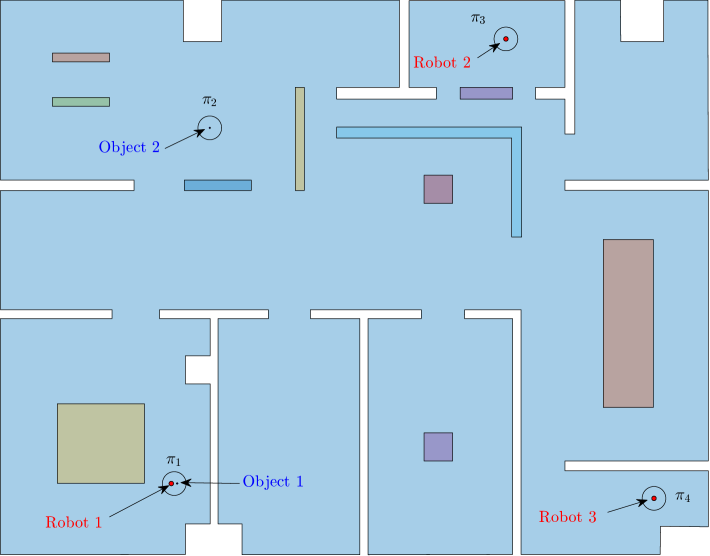
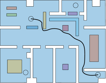
In this case study, we consider robots, regions and objects. The regions of interest are circular centered at m, m, m, and m, with radius equal to m. The robots’ and object’ mass is taken as kg and kg, respectively, while their spherical volume’s radii as m and m, respectively. The power capabilities of the robots are , respectively, and the power required for each object is , respectively. Initially, the robots are located in regions , , and , respectively, whereas the objects are located in regions , , respectively. Fig. 1 depicts the considered environment and the initial configuration of the multi-robot-object system.
The resulting transition system consists of reachable states and transitions and it was created within minutes. We set the following formula for the multi-robot-object system:
| (13) |
with
-
•
-
•
-
•
-
•
-
•
In words, the mission specification in (13) requires the robots and objects to satisfy , , and infinitely often, satisfy eventually, and satisfy before satisfying . The LTL formula in (13) corresponds to a NBA with states - among which one is a final state - and transitions. STyLuS* found the first feasible prefix and suffix path within minutes and minutes on average. The action path of the robots is depicted in Table I, starting from and satisfying .
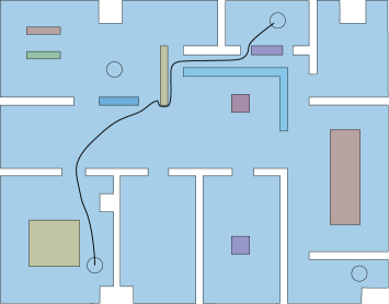
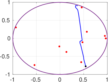
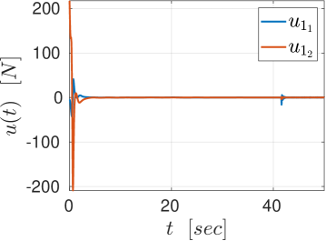
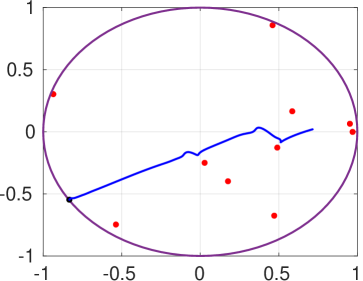
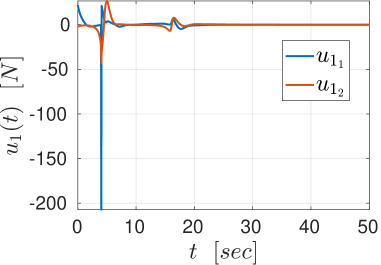
We further illustrate the continuous control design. In particular, we consider the actions of robot navigation and object transportation. Firstly, we examine the navigation of robot 1 from to . The results are depicted in Figs. 2, 3. The left part of Fig. 2 shows the trajectory of robot in the environment, where the obstacles and boundary have absorbed the the spherical volume of the robot; the right part of Fig. 2 shows the trajectory of robot in the transformed point world, where the obstacles are represented by points. Fig. 3 depicts the control input (left) and the evolution of the adaptation signals , (right).
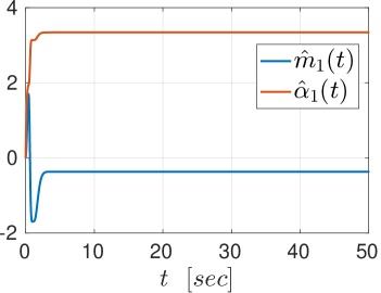
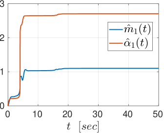
We further examine the transportation of object by robots and from to , where we chose the load-sharing coefficients . The results are depicted in Figs. 4, 5. The left part of Fig. 4 shows the trajectory of the coupled object-robots system in the environment, where the obstacles and boundary have absorbed the its spherical volume; the right part of Fig. 2 shows the trajectory of the coupled system in the transformed point world, where the obstacles are represented by points. Fig. 3 depicts the control input (left) and the evolution of the adaptation signals , (right) of the robot 1, which are identical to the ones of robot 2.
| Actions | Actions | ||
|---|---|---|---|
| , , | |||
| , | , | ||
| , | |||
| , | |||
| , | , , | ||
| , , | |||
| , | |||
| , | |||
| , | |||
| , | , | ||
| , | , | ||
| , | |||
| , , | |||
| , , | |||
| , | |||
| , | , , | ||
| , | |||
| , | , | ||
| , , | |||
| , , | |||
| , | |||
| , | , | ||
| , | , | ||
| , | , | ||
| , , | |||
| , , | |||
| , , | |||
| , | |||
| , | |||
| , | |||
| , , | |||
IV-B Case Study II:
In this case study, we consider robots, regions and objects. The regions of interest are circular centered at m, m, and m, with radius equal to m, as in the previous case study. The robots’ and object’ mass is taken as kg and kg, respectively, while their spherical volume’s radii as m and m, respectively. The power capabilities of the robots are , respectively, and the power required for each object is , respectively. Initially, the robots are located in regions , , , and , respectively, whereas the objects are located in regions , , and , respectively.
The resulting transition system consists of reachable states and transitions and it was created within 1.52 hours. We set the following formula for the multi-robot-object system:
| (14) |
with
-
•
-
•
-
•
-
•
-
•
-
•
-
•
-
•
The LTL formula in (IV-B) corresponds to a NBA with states - among which one is a final state - and transitions. STyLuS* found the first feasible prefix and suffix path within minutes and minutes on average. We omit the action path of the robots for ease of exposition.
V Conclusion
We propose an algorithm for the control and planning of multi-robot-object systems subject LTL tasks. We develop adaptive feedback-control protocols for robot navigation and cooperative object transportation, which enable the abstraction of the underlying continuous dynamics to a finite transition system. We compose the transition system with an automaton that represents the LTL task and use a sampling-based planner to derive an optimal task-satisfying plan for the robots.
References
- [1] G. E. Fainekos, A. Girard, H. Kress-Gazit, and G. J. Pappas, “Temporal logic motion planning for dynamic robots,” Automatica, vol. 45, no. 2, pp. 343–352, 2009.
- [2] M. Lahijanian, M. R. Maly, D. Fried, L. E. Kavraki, H. Kress-Gazit, and M. Y. Vardi, “Iterative temporal planning in uncertain environments with partial satisfaction guarantees,” IEEE Transactions on Robotics, vol. 32, no. 3, pp. 583–599, 2016.
- [3] S. G. Loizou and K. J. Kyriakopoulos, “Automatic synthesis of multi-agent motion tasks based on ltl specifications,” IEEE Conference on Decision and Control (CDC), vol. 1, pp. 153–158, 2004.
- [4] Y. Diaz-Mercado, A. Jones, C. Belta, and M. Egerstedt, “Correct-by-construction control synthesis for multi-robot mixing,” IEEE Conference on Decision and Control (CDC), pp. 221–226, 2015.
- [5] Y. Chen, X. C. Ding, A. Stefanescu, and C. Belta, “Formal approach to the deployment of distributed robotic teams,” IEEE Transactions on Robotics, vol. 28, no. 1, pp. 158–171, 2012.
- [6] R. V. Cowlagi and Z. Zhang, “Motion-planning with linear temporal logic specifications for a nonholonomic vehicle kinematic model,” American Control Conference (ACC), pp. 6411–6416, 2016.
- [7] C. Belta, V. Isler, and G. J. Pappas, “Discrete abstractions for robot motion planning and control in polygonal environments,” IEEE Transactions on Robotics, vol. 21, no. 5, pp. 864–874, 2005.
- [8] A. Bhatia, M. R. Maly, L. E. Kavraki, and M. Y. Vardi, “Motion planning with complex goals,” IEEE Robotics & Automation Magazine, vol. 18, no. 3, pp. 55–64, 2011.
- [9] I. Filippidis, D. V. Dimarogonas, and K. J. Kyriakopoulos, “Decentralized multi-agent control from local ltl specifications,” IEEE Conference on Decision and Control (CDC), pp. 6235–6240, 2012.
- [10] M. Guo and D. V. Dimarogonas, “Multi-agent plan reconfiguration under local ltl specifications,” The International Journal of Robotics Research, vol. 34, no. 2, pp. 218–235, 2015.
- [11] C. Belta and L. C. Habets, “Controlling a class of nonlinear systems on rectangles,” IEEE Transactions on Automatic Control, vol. 51, no. 11, pp. 1749–1759, 2006.
- [12] G. Reißig, “Computing abstractions of nonlinear systems,” IEEE Transactions on Automatic Control, vol. 56, no. 11, pp. 2583–2598, 2011.
- [13] A. Tiwari, “Abstractions for hybrid systems,” Formal Methods in System Design, vol. 32, no. 1, pp. 57–83, 2008.
- [14] M. Rungger, A. Weber, and G. Reissig, “State space grids for low complexity abstractions,” IEEE Conference on Decision and Control (CDC), pp. 6139–6146, 2015.
- [15] D. Boskos and D. V. Dimarogonas, “Decentralized abstractions for feedback interconnected multi-agent systems,” IEEE Conference on Decision and Control (CDC), pp. 282–287, 2015.
- [16] C. Belta and V. Kumar, “Abstraction and control for groups of robots,” IEEE Transactions on robotics, vol. 20, no. 5, pp. 865–875, 2004.
- [17] T. G. Sugar and V. Kumar, “Control of cooperating mobile manipulators,” IEEE Transactions on robotics and automation, vol. 18, no. 1, pp. 94–103, 2002.
- [18] D. Heck, D. Kostic, A. Denasi, and H. Nijmeijer, “Internal and external force-based impedance control for cooperative manipulation,” pp. 2299–2304, 2013.
- [19] Y. Kume, Y. Hirata, and K. Kosuge, “Coordinated motion control of multiple mobile manipulators handling a single object without using force/torque sensors,” IEEE/RSJ International Conference on Intelligent Robots and Systems (IROS), pp. 4077–4082, 2007.
- [20] A. Tsiamis, C. K. Verginis, C. P. Bechlioulis, and K. J. Kyriakopoulos, “Cooperative manipulation exploiting only implicit communication,” IEEE/RSJ International Conference on Intelligent Robots and Systems (IROS), pp. 864–869, 2015.
- [21] F. Ficuciello, A. Romano, L. Villani, and B. Siciliano, “Cartesian impedance control of redundant manipulators for human-robot co-manipulation,” IEEE/RSJ International Conference on Intelligent Robots and Systems (IROS), pp. 2120–2125, 2014.
- [22] A.-N. Ponce-Hinestroza, J.-A. Castro-Castro, H.-I. Guerrero-Reyes, V. Parra-Vega, and E. Olguín-Díaz, “Cooperative redundant omnidirectional mobile manipulators: Model-free decentralized integral sliding modes and passive velocity fields,” IEEE International Conference on Robotics and Automation (ICRA), pp. 2375–2380, 2016.
- [23] A. Marino, “Distributed adaptive control of networked cooperative mobile manipulators,” IEEE Transactions on Control Systems Technology, 2017.
- [24] A. Nikou, C. Verginis, S. Heshmati-Alamdari, and D. V. Dimarogonas, “A nonlinear model predictive control scheme for cooperative manipulation with singularity and collision avoidance,” Mediterranean Conference on Control and Automation (MED), pp. 707–712, 2017.
- [25] C. K. Verginis, A. Nikou, and D. V. Dimarogonas, “Communication-based decentralized cooperative object transportation using nonlinear model predictive control,” European control conference (ECC), pp. 733–738, 2018.
- [26] C. K. Verginis, M. Mastellaro, and D. V. Dimarogonas, “Robust cooperative manipulation without force/torque measurements: Control design and experiments,” IEEE Transactions on Control Systems Technology, vol. 28, no. 3, pp. 713–729, 2019.
- [27] S. Erhart and S. Hirche, “Model and analysis of the interaction dynamics in cooperative manipulation tasks,” IEEE Transactions on Robotics, vol. 32, no. 3, pp. 672–683, 2016.
- [28] H. G. Tanner, S. G. Loizou, and K. J. Kyriakopoulos, “Nonholonomic navigation and control of cooperating mobile manipulators,” IEEE Transactions on robotics and automation, vol. 19, no. 1, pp. 53–64, 2003.
- [29] C. K. Verginis and D. V. Dimarogonas, “Timed abstractions for distributed cooperative manipulation,” Autonomous Robots, pp. 1–19, 2017.
- [30] ——, “Multi-agent motion planning and object transportation under high level goals,” IFAC World Congress, 2017.
- [31] C. Baier, J.-P. Katoen, and K. G. Larsen, Principles of model checking. MIT press, 2008.
- [32] C. Makkar, W. Dixon, W. Sawyer, and G. Hu, “A new continuously differentiable friction model for control systems design,” IEEE/ASME International Conference on Advanced Intelligent Mechatronics, pp. 600–605, 2005.
- [33] D. Z. Chen, “Sphere packing problem,” Encyclopedia of Algorithms, pp. 1–99, 2008.
- [34] M. R. Cutkosky, Robotic grasping and fine manipulation. Springer Science & Business Media, 2012, vol. 6.
- [35] M. F. Reis, A. C. Leite, and F. Lizarralde, “Modeling and control of a multifingered robot hand for object grasping and manipulation tasks,” IEEE Conference on Decision and Control (CDC), pp. 159–164, 2015.
- [36] C. K. Verginis and D. V. Dimarogonas, “Adaptive robot navigation with collision avoidance subject to 2nd-order uncertain dynamics,” Automatica, vol. 123, p. 109303, 2021.
- [37] P. Vlantis, C. Vrohidis, C. P. Bechlioulis, and K. J. Kyriakopoulos, “Robot navigation in complex workspaces using harmonic maps,” IEEE International Conference on Robotics and Automation (ICRA), pp. 1726–1731, 2018.
- [38] S. L. Smith, J. Tumova, C. Belta, and D. Rus, “Optimal path planning for surveillance with temporal-logic constraints,” The International Journal of Robotics Research, vol. 30, no. 14, pp. 1695–1708, 2011.
- [39] A. Ulusoy, S. L. Smith, and C. Belta, “Optimal multi-robot path planning with ltl constraints: guaranteeing correctness through synchronization,” in Distributed Autonomous Robotic Systems. Springer, 2014, pp. 337–351.
- [40] Y. Kantaros and M. M. Zavlanos, “Stylus*: A temporal logic optimal control synthesis algorithm for large-scale multi-robot systems,” The International Journal of Robotics Research, vol. 39, no. 7, pp. 812–836, 2020.