Point Cloud Pre-training with Diffusion Models
Abstract
Pre-training a model and then fine-tuning it on downstream tasks has demonstrated significant success in the 2D image and NLP domains. However, due to the unordered and non-uniform density characteristics of point clouds, it is non-trivial to explore the prior knowledge of point clouds and pre-train a point cloud backbone. In this paper, we propose a novel pre-training method called Point cloud Diffusion pre-training (PointDif). We consider the point cloud pre-training task as a conditional point-to-point generation problem and introduce a conditional point generator. This generator aggregates the features extracted by the backbone and employs them as the condition to guide the point-to-point recovery from the noisy point cloud, thereby assisting the backbone in capturing both local and global geometric priors as well as the global point density distribution of the object. We also present a recurrent uniform sampling optimization strategy, which enables the model to uniformly recover from various noise levels and learn from balanced supervision. Our PointDif achieves substantial improvement across various real-world datasets for diverse downstream tasks such as classification, segmentation and detection. Specifically, PointDif attains 70.0% mIoU on S3DIS Area 5 for the segmentation task and achieves an average improvement of 2.4% on ScanObjectNN for the classification task compared to TAP. Furthermore, our pre-training framework can be flexibly applied to diverse point cloud backbones and bring considerable gains.
1 Introduction
In recent years, a surging number of studies, including SAM [19], VisualChatGPT [53], and BLIP-2 [21], have demonstrated the exceptional performance of pre-trained models across a broad range of 2D image and natural language processing (NLP) tasks. Pre-training on large-scale datasets endows the model with abundant prior knowledge, enabling the pre-trained models to exhibit superior performance and enhanced generalization capabilities after finetuning, compared to models trained solely on downstream tasks [18, 31, 21]. Similar to the 2D and NLP fields, pre-training methods in point cloud data have also become essential in enhancing model performance and boosting model generalization ability.
Contemporary point cloud pre-training methods can be casted into two categories, i.e., contrastive-based and generative-based pre-training. Contrastive-based methods [55, 61, 1] resort to the contrastive objective to make deep models grasp the similarity knowledge between samples. By contrast, generative-based methods involve pre-training by reconstructing the masked point cloud [31, 60] or its 2D projections [49, 15]. However, several factors mainly account for the inferior pre-training efficacy in the 3D domain. For contrastive-based methods [55, 1], selecting the proper negative samples to construct the contrastive objective is non-trivial. The generative-based pre-training approaches, such as Point-MAE [31] and Point-M2AE [60], solely reconstruct the masked point patches. In this way, they cannot capture the global density distribution of the object. Additionally, there is no precise one-to-one matching for MSE loss and set-to-set matching for Chamfer Distance loss between reconstructed and original point cloud due to its unordered nature. Besides, the projection from 3D to 2D by TAP [49] and Ponder [15] inevitably introduces the geometric information loss, making the reconstruction objective difficult to equip the backbone with comprehensive geometric prior.
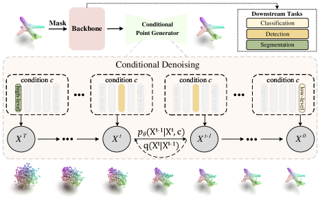
To combat against the unordered and non-uniform density characteristics of point clouds, inspired by adding noise and denoising of the diffusion model [14], we propose a novel diffusion-based pre-training framework, dubbed PointDif. It pre-trains the point cloud backbone by restoring the noisy data at each step as illustrated in Fig. 1. This procedural denoising process is similar to the visual streams in our human brain mechanism [41]. Human uses this simple brain mechanism to obtain broad prior knowledge from the 3D world. Similarly, we find that low-level and high-level neural representation emerges from denoising neural networks. This aligns with our goal of applying pre-trained models to downstream low-level and high-level tasks, such as classification and segmentation. Moreover, the diffusion model has strong theoretical guarantees and provides an inherently hierarchical learning strategy by enabling the understanding of data distribution hierarchically.
Specifically, we present a conditional point generator in our PointDif, which guides the point-to-point generation from the noisy point cloud. This conditional point generator encompasses a Condition Aggregation Network (CANet) and a Conditional Point Diffusion Model (CPDM). The CANet is responsible for globally aggregating latent features extracted by the backbone. The aggregated features serve as the condition to guide the CPDM in denoising the noisy point cloud. During the denoising process, the point-to-point mapping relationship exists in the noisy point cloud at neighboring time steps. Equipped with the CPDM, the backbone can effectively capture the global point density distribution of the object. This enables the model to adapt to downstream tasks that involve point clouds with diverse density distributions. With the help of the conditional point generator, our pre-training framework can be extended to various point cloud backbones and enhance their overall performance.
Moreover, as shown in Tab. 8, we find that sampling time step from different intervals during pre-training can learn different levels of geometric prior. Based on this observation, we propose a recurrent uniform sampling optimization strategy. This strategy divides the diffusion time steps into multiple intervals and uniformly samples the time step throughout the pre-training process. In this way, the model can uniformly recover from various noise levels and learn from balanced supervision. To the best of our knowledge, we are the first to demonstrate the effectiveness of generative diffusion models in enhancing point cloud pre-training.
Our key contributions can be summarized as follows:
-
•
We propose the first framework for point cloud pre-training based on diffusion models, called PointDif. Performing iterative denoising on the noisy point cloud can assist backbones in acquiring a comprehensive understanding of the original point cloud and extracting hierarchical geometric prior.
-
•
We present a conditional point generator to guide the point-to-point generation from the noisy point cloud. This facilitates the network in capturing the global point density distribution of the object.
-
•
We introduce a recurrent uniform sampling strategy that assists the model in uniformly restoring diverse noise levels and learning from balanced supervision.
-
•
Our PointDif demonstrates competitive performance across various real-world downstream tasks. Furthermore, our framework can be flexibly applied to diverse point cloud backbones and enhance their performance.
2 Related Work
This section first briefly reviews existing point cloud pre-training approaches. Since the diffusion model is a primary component in the proposed pre-training framework, we also review the relevant studies on diffusion models.
Pre-training for 3D point cloud. Contrastive-based algorithms pre-train the backbone by comparing the similarities and differences among samples. PointContrast [55] is the pioneering method, which constructs two point clouds from different perspectives and compares point feature similarities for point cloud pre-training. Recent research efforts have improved network performance through data augmentation [61, 54] and the introduction of cross-modal information [1, 17, 59]. In contrast, generative-based pre-training methods focus on pre-training the encoder by recovering masked information or its 2D projections. Point-BERT [58] and Point-MAE [31] respectively incorporate the ideas of BERT [10] and MAE [13] into point cloud pre-training. TAP [49] and Ponder [15] pre-train the point cloud backbone by generating the 2D projections of the point cloud. Point-M2AE [60] constructs a hierarchical network capable of gradually modeling geometric and feature information. Joint-MAE [12] focuses on the correlation between 2D images and 3D point cloud and introduces hierarchical modules for cross-modal interaction to reconstruct masked information for both modalities. Compared to the architectural improvements made in Point-M2AE and Joint-MAE, our method concentrates on refining the training approach. Our PointDif leverages the progressive guidance characteristic of the conditional diffusion model, allowing the backbone to learn hierarchical geometric prior by restoring noisy point clouds at different noise levels.
Diffusion Probabilistic Models. The diffusion model is inspired by the principles of non-equilibrium thermodynamics and leverages the diffusion process and noise reduction to generate high-quality data. It has shown excellent performance in both generation effectiveness and interpretability. The diffusion model has achieved remarkable success across various domains, including image generation [30, 11, 37, 39, 38, 62] and 3D generation [23, 57, 43, 48, 25]. Recently, researchers have investigated methods for accelerating the sampling process of DDPM to improve its generation efficiency [40, 26, 27]. Moreover, some studies have explored the application of diffusion models in discriminative tasks, such as object detection[7] and semantic segmentation [2, 51, 4].
To our knowledge, we are the first to apply the diffusion model for point cloud pre-training and have achieved promising results. The most relevant work is the 2D pre-training method DiffMAE [50]. However, there are four critical distinctions between our PointDif and DiffMAE. Firstly, as to the reconstruction target, DiffMAE pre-trains the network by denoising pixel values of masked patches. In contrast, our PointDif pre-trains the network by recovering the original point clouds from randomly noisy point clouds, which is beneficial for the network to learn both local and global geometrical priors of 3D objects. Secondly, as for the guidance way, DiffMAE uses the conditional guidance method of cross-attention. We adopt a point condition network (PCNet) for point cloud data to facilitate 3D generation through point-by-point guidance. It also assists the network in learning the global point density distribution of the object. Thirdly, regarding the loss function, DiffMAE introduces an additional CLIP loss to constrain the model, whereas our PointDif demonstrates strong performance in various 3D downstream tasks without additional constraints. Finally, with regard to the unity of the framework, DiffMAE can only pre-train the 2D transformer encoder. In comparison, with the help of our conditional point generator, we can pre-train various point cloud backbones and enhance their performance.
3 Methodology
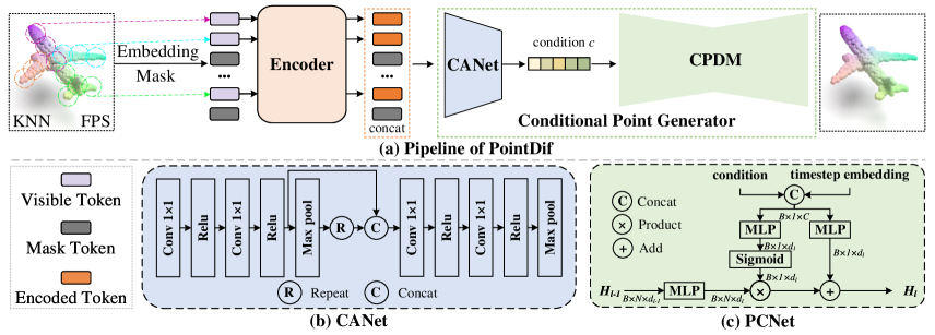
We take pre-training the transformer encoder as an example to introduce our overall pre-training framework, i.e., PointDif. The framework can also be easily applied to pre-train other backbones. The pipeline of our PointDif is shown in Fig. 2a. Given a point cloud, we first divide it into point patches and apply embedding and random masking operations to each patch. Subsequently, we use a transformer encoder to process visible tokens to learn the latent features, which are then used to generate the condition through the CANet. Finally, this condition gradually guides the CPDM to recover the original input point cloud from the random noise point cloud in a point-to-point manner. We pre-train the transformer encoder to acquire the hierarchical geometric prior through the progressively guided process.
3.1 Preliminary: Conditional Point Diffusion
During the diffusion process, random noise is continuously introduced into the point cloud through a Markov chain, and there exists a point-to-point mapping relationship between noisy point clouds of adjacent timestamps. Formally, given a clean point cloud containing points from the real data distribution , the diffusion process gradually adds Gaussian noise to for time steps:
| (1) |
| (2) |
the hyperparameters are some pre-defined small constants and gradually increase over time. is sampled from a Gaussian distribution with mean and variance . Moreover, according to [14], it is possible to elegantly express as a direct function of :
| (3) |
where and . As the time step increases, gradually approaches 0 and will be close to the Gaussian distribution .
The reverse process involves using a neural network parameterized by to gradually denoise a Gaussian noise into a clean point cloud with the help of the condition . This process can be defined as:
| (4) |
| (5) |
the is a neural network that predicts the mean, and is a constant that varies with time.
The training objective of the diffusion model is formulated based on variational inference, which employs the variational lower bound () to optimize the negative log-likelihood:
| (6) |
where is the KL divergence. However, training is prone to instability. To address this, we adopt a simplified version of the mean squared error [14]:
| (7) |
where , is a trainable neural network that takes the noisy point cloud at time , along with the time and condition as inputs. This network predicts the added noise . Additional details regarding derivations and proofs can be found in Sec. 6.
3.2 Point Cloud Processing
The goal of point cloud processing is to convert the given point cloud into several tokens, which consist of point patch embedding and patch masking.
Point Patch Embedding. Following Point-BERT [58] and Point-MAE [31], we divide the point cloud into point patches using a grouping strategy. Specifically, for an input point cloud consisting of points, we first employ the Farthest Point Sampling (FPS) algorithm to sample center points . For each center point , we use the K Nearest Neighborhood (KNN) algorithm to gather the nearest points as a point patch .
| (8) |
It is noteworthy that we apply a centering process to the point patches, which involves subtracting the coordinates of the point center from each point within the patch. This operation helps improve the convergence of the model. Subsequently, we utilize a simplified PointNet [32] with parameter , which employs convolutions and max pooling, to embed the point patches into tokens .
| (9) |
Patch Masking. In order to preserve the geometric information within the patch, we randomly mask the entire points in the patch to obtain the masked tokens and visible tokens , where is the number of masked tokens, is the number of visible tokens, is the floor operation and denotes the masking ratio. We conduct experiments to assess the impact of different masking ratios and find that higher masking ratios (0.7-0.9) result in better performance, as discussed in Sec. 4.3.
3.3 Encoder
The transformer encoder is responsible for extracting latent geometric features, which is retained for feature extraction during fine-tuning for downstream tasks. is our encoder with parameter , composed of 12 standard transformer blocks. To better capture meaningful 3D geometric prior, we remove the masked tokens and encode only the visible tokens . Furthermore, we introduce a position embedding with parameter to embed the position information of the point patch into , which is comprised of two learnable MLPs and the GELU activation function. Then, the position embedding output is concatenated with and sent through a sequence of transformer blocks for feature extraction.
| (10) |
| (11) |
3.4 Conditional Point Generator
Our conditional point generator consists of the CANet and the CPDM.
Condition Aggregation Network (CANet). To be specific, we concatenate features of the visible patches extracted by the encoder with a set of learnable masked patch information , while preserving their original position information. Afterward, the concatenated features are encoded using the CANet, denoted as with the parameter . As shown in Fig. 2b, our CANet consists of four 1x1 convolutional layers and two global max-pooling layers to aggregate the global contextual features of the point cloud. Ultimately, this process yields the guiding condition required for the CPDM:
| (12) |
Conditional Point Diffusion Model (CPDM). Inspired by [28], we adopt a point diffusion model, which utilizes the condition to guide the recovery of the original point cloud from a randomly perturbed point cloud in a point-to-point way. As illustrated in Fig. 2c, the conditional point diffusion model comprises six point condition network (PCNet). The specific structure of each PCNet can be represented as follows:
| (13) |
where and are respectively the input and output of PCNet, represents the sigmoid function, and are all trainable parameters. represents the feature obtained by concatenating the condition with the time step embedding. The input dimensions for each PCNet are [3, 128, 256, 512, 256, 128] and the output dimension of the last PCNet is 3. By incorporating the condition into the control mechanism of the reset gate , the model can adaptively select geometric features to denoise. Recovering from noisy point clouds through point-to-point guidance can aid the network in learning the overall point density distribution of the object. This, in turn, assists different backbones in learning a broader range of dense and sparse geometric priors, resulting in enhanced performance in downstream tasks related to indoor and outdoor scenes.
3.5 Training Objective
We introduce the process of encoding condition into Eq. 7. Therefore, the training objective of our model can be defined as follows:
| (14) |
By minimizing this loss, we can simultaneously train the encoder , the CANet and the CPDM . Intuitively, the training process encourages the encoder to extract hierarchical geometric features from the original point cloud and encourages the CPDM to reconstruct the original point cloud according to the hierarchical geometric features. In this process, the CPDM performs a task similar to point cloud completion.
| Methods | Pre. | OBJ-ONLY | OBJ-BG | PB-T50-RS |
|---|---|---|---|---|
| PointNet [32] | ✘ | 79.2 | 73.3 | 68.0 |
| PointNet++ [33] | ✘ | 84.3 | 82.3 | 77.9 |
| PointCNN [22] | ✘ | 85.5 | 86.1 | 78.5 |
| DGCNN [47] | ✘ | 86.2 | 82.8 | 78.1 |
| Transformer [58] | ✘ | 80.55 | 79.86 | 77.24 |
| Transformer-OcCo [58] | ✘ | 85.54 | 84.85 | 78.79 |
| Point-BERT [58] | ✔ | 88.12 | 87.43 | 83.07 |
| MaskPoint [24] | ✔ | 89.70 | 89.30 | 84.60 |
| Point-MAE [31] | ✔ | 88.29 | 90.02 | 85.18 |
| TAP [49] | ✔ | 89.50 | 90.36 | 85.67 |
| PointDif (Ours) | ✔ | 91.91 | 93.29 | 87.61 |
Recurrent Uniform Sampling Strategy. According to Eq. 14, we need to sample a time step randomly from the range [1, T] for each point cloud data for network training. However, we observe that networks trained with samples from different time steps exhibit varying performance on downstream tasks. As illustrated in Tab. 8, the encoder trained by sampling from the early interval is more suitable for the classification task. In contrast, the encoder trained by sampling from the later interval performs better on the segmentation task. Based on this discovery, We propose a more effective recurrent uniform sampling strategy. Specifically, we divide the time step range [1, T] into intervals: where . As in Eq. 15, we randomly sample from these intervals for each sample data, calculate the loss times, and average them to obtain the final loss.
| (15) |
Intuitively, this sampling strategy allows the encoder to learn different levels of geometric prior and learn from balanced supervision. It is more uniform compared to randomly sampling a single from in the original DDPM [14]. Our approach divides the time steps into = 4 intervals, as discussed in Sec. 4.3.
Discussion. We chose to pre-train the backbone instead of the diffusion model for two reasons. Firstly, the backbone can be various deep feature extraction networks, which is more effective in extracting low-level and high-level geometric features compared to the typically simpler diffusion model . Secondly, separating the backbone from the pipeline makes our pre-trained framework more adaptable to different architectures, thereby increasing its flexibility.
| Methods | Pre. | Pre Dataset | |
|---|---|---|---|
| VoteNet [34] | ✘ | - | 33.5 |
| STRL [16] | ✔ | ScanNet [9] | 38.4 |
| PointContrast [55] | ✔ | ScanNet [9] | 38.0 |
| DepthContrast [61] | ✔ | ScanNet-vid [61] | 42.9 |
| 3DETR [29] | ✘ | - | 37.9 |
| Point-BERT [58] | ✔ | ScanNet-Medium [24] | 38.3 |
| MaskPoint [24] | ✔ | ScanNet-Medium [24] | 42.1 |
| Point-MAE [31] | ✔ | ShapeNet [6] | 42.8 |
| TAP [49] | ✔ | ShapeNet [6] | 41.4 |
| PointDif (Ours) | ✔ | ShapeNet [6] | 43.7 |
4 Experiments
4.1 Pre-training Setups
Pre-training. We use ShapeNet [6] to pre-train the model, a synthetic 3D dataset that contains 52,470 3D shapes across 55 object categories. We pre-train our model only on the training set, which consists of 41,952 shapes. For each 3D shape, we sample 1,024 points to serve as the input for the model. We set as 64, which means each point cloud is divided into 64 patches. Furthermore, the KNN algorithm is used to select =32 nearest points as a point patch.
Model Configurations. Following [58, 31], we set the embedding dimension of the transformer encoder to 384 and the number of heads to 6. The condition dimension is 768.
Training Details. During pre-training, we adopt the AdamW optimizer with a weight decay of 0.05 and a learning rate of 0.001. We apply the cosine decay schedule to adjust the learning rate. Random scaling and translation are used for data augmentation. Our model is pre-trained for 300 epochs with a batchsize of 128. The for the diffusion process is set to 2000, and linearly increases from 1e-4 to 1e-2.
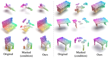
Visualization. To demonstrate the effectiveness of our pre-training scheme, we visualize the point cloud generated by our PointDif. As shown in Fig. 3, we apply a high mask ratio of 0.8 to the input point cloud for masking and use the masked point cloud as a condition to guide the diffusion model in generating the original point cloud. Our PointDif produces high-quality point clouds. Experimental results demonstrate that the geometric prior learned through our pre-training method can provide excellent guidance for both shallow texture and shape semantics.
| Methods | Pre. | mIoU | mAcc |
|---|---|---|---|
| PointNet [32] | ✘ | 41.1 | 49.0 |
| PointNet++ [33] | ✘ | 53.5 | - |
| PointCNN [22] | ✘ | 57.3 | 63.9 |
| KPConv [44] | ✘ | 67.1 | 72.8 |
| SegGCN [20] | ✘ | 63.6 | 70.4 |
| Pix4Point [36] | ✘ | 69.6 | 75.2 |
| MKConv [52] | ✘ | 67.7 | 75.1 |
| PointNeXt [35] | ✘ | 68.5 | 75.1 |
| Point-BERT [58] | ✔ | 68.9 | 76.1 |
| MaskPoint [24] | ✔ | 68.6 | 74.2 |
| Point-MAE [31] | ✔ | 68.4 | 76.2 |
| PointDif (Ours) | ✔ | 70.0 | 77.1 |
4.2 Downstream Tasks
A high-quality point cloud pre-trained model should perceive hierarchical geometric prior. To assess the efficacy of the pre-trained model, we gauged its performance on various fine-tuned tasks using numerous real-world datasets.
| Methods | mIoU | car | bicycle | truck | preson | bicyclist | motorcyclist | road | sidewalk | parking | vegetation | trunk | terrain |
|---|---|---|---|---|---|---|---|---|---|---|---|---|---|
| Cylinder3D [63] | 66.1 | 96.9 | 54.4 | 81.0 | 79.3 | 92.4 | 0.1 | 94.6 | 82.2 | 47.9 | 85.9 | 66.9 | 69.2 |
| SPVCNN [42] | 68.6 | 97.9 | 59.8 | 79.8 | 80.0 | 92.0 | 0.6 | 94.2 | 81.7 | 50.4 | 88.0 | 69.7 | 74.1 |
| RPVNet [56] | 68.9 | 97.9 | 42.8 | 91.2 | 78.3 | 90.2 | 0.7 | 95.2 | 83.1 | 57.1 | 87.3 | 71.4 | 72.0 |
| MinkowskiNet [8] | 70.2 | 97.4 | 56.1 | 84.0 | 81.9 | 91.4 | 24.0 | 94.0 | 81.3 | 52.2 | 88.4 | 68.6 | 74.8 |
| MinkowskiNet+PointDif | 71.3 | 97.5 | 58.8 | 92.8 | 81.4 | 92.3 | 30.3 | 94.1 | 81.7 | 56.0 | 88.5 | 69.1 | 75.2 |
| Methods | ||
|---|---|---|
| CAGroup [46] | 73.20 | 60.84 |
| CAGroup+PointDif | 74.14 | 61.31 |
Object Classification. We first use the classification task on ScanObjectNN [45] to evaluate the shape recognition ability of the pre-trained model by PointDif. The ScanObjectNN dataset is divided into three subsets: OBJ-ONLY (only objects), OBJ-BG (objects and background), and PB-T50-RS (objects, background, and artificially added perturbations). We take the Overall Accuracy on these three subsets as the evaluation metric, and the detailed experimental results are summarized in Tab. 1. Our PointDif achieves better performance on all subsets, exceeding TAP by 2.4, 2.9 and 1.9, respectively. The significant improvement on the challenging ScanObjectNN benchmark strongly validates the effectiveness of our model in shaping understanding.
Object Detection. We validate our model on the more challenging indoor dataset ScanNetV2 [9] for 3D object detection task to assess the scene understanding ability. We adopt 3DETR [29] as our method’s task head. To ensure a fair comparison, we follow MaskPoint [24] and replace the encoder of 3DETR with our pre-trained encoder and fine-tune it. Unlike MaskPoint and Point-BERT, which are pre-trained on the ScanNet-Medium dataset in the same domain as ScanNetV2, our approach and Point-MAE are pre-trained on ShapeNet in a different domain and only fine-tuned on the training set of ScanNetV2. Tab. 2 displays our experimental results. Our method outperforms Point-MAE and surpasses MaskPoint and Point-BERT by 1.6% and 5.4%, respectively. Additionally, our approach exhibits a 2.3% improvement compared to pre-training the transformer encoder of 3DETR on the ShapeNet dataset using the TAP method. The experiments demonstrate that our model exhibits strong transferability and generalization capability on scene understanding.
Indoor Semantic Segmentation. We further validate our model on the indoor S3DIS dataset [3] for semantic segmentation tasks to show the understanding of contextual semantics and local geometric relationships. We test our model on Area 5 while training on other areas. To make a fair comparison, we put all pre-trained models in the same codebase based on the PointNext [35] baseline and use the same decoder and semantic segmentation head. We freeze the encoder pre-trained on ShapeNet and fine-tune the decoder and the segmentation head. The experiment results are shown in Tab. 3. Compared to training from scratch, our method boosts the performance of PointNext by 1.5% in terms of mIoU. Compared to other pre-training methods such as Point-BERT, MaskPoint and Point-MAE, our method achieves approximately 1.4% improvement for each on mIoU. Note that, PointNext is originally trained using a batchsize of 8, since computational resource constraints, we thus retrained it with a batchsize of 4 for a fair comparison. Significant improvements indicate that our pre-trained model has successfully acquired hierarchical geometric prior knowledge essential for comprehending contextual semantics and local geometric relationships.
| Methods | mIoU | mAcc |
|---|---|---|
| Cross Attention | 69.09 | 75.19 |
| Point Concat | 69.43 | 75.39 |
| Point Condition Network | 70.02 | 77.05 |
Outdoor Semantic Segmentation. We also validate the effectiveness of our method on the more challenging real-world outdoor scene dataset KITTI. The SemanticKITTI dataset [5] is a large-scale outdoor LiDAR segmentation dataset, consisting of 43,000 scans with 19 semantic categories. We employ MinkowskiNet [8] as our baseline model. During the pre-training phase, we discard its segmentation head and utilize the backbone MinkUNet as the encoder to extract latent features. We pre-train the MinkUNet using our framework on ShapeNet and subsequently fine-tuned it on the SemanticKITTI. Other pre-training configurations follow the guidelines outlined in Sec. 4.1. The experiment results in Tab. 4 demonstrate that our pre-training method achieves 71.3% mIoU, which is a 1.1% improvement over the train-from-scratch variant. Our pre-training framework for point-to-point guided generation can assist the backbone in learning density priors and enable it to adapt to downstream tasks with significant density variations. The entire results are reported in Sec. 8.
Object detection results of CAGroup3D with and without pre-training. We further evaluate our pre-training method on the competitive 3D object detection model, CAGroup3D [46], a two-stage fully sparse 3D detection network. We train CAGroup3D from scratch and report the result for a fair comparison. We use our method to pre-train the backbone BiResNet on ShapeNet. Specifically, we treat BiResNet as the encoder to extract features. The conditional point generator employs the masked features to guide the point-to-point recovery of the original point cloud. Other pre-training settings follow Sec. 4.1. The experimental results are shown in Tab. 5. Compared to the train-from-scratch variant, our method improves performance by 0.9% and 0.5% on and , respectively. Therefore, our pre-training framework can be flexibly applied to various backbones to improve performance. Please refer to Sec. 8 for additional results.
| #Point Clouds | # | Intervals | Effective Batchsize | mIoU | mAcc |
| 128 | 4 | 4 | 512 | 70.02 | 77.05 |
| 128 | 4 | 1 | 512 | 69.68 | 75.90 |
| 256 | 2 | 2 | 512 | 69.67 | 76.26 |
| 256 | 2 | 1 | 512 | 69.36 | 75.94 |
| 64 | 8 | 8 | 512 | 69.42 | 75.71 |
| 64 | 8 | 1 | 512 | 69.24 | 75.50 |
| 512 | 1 | 4 | 512 | 69.91 | 75.93 |
| 512 | 1 | 1 | 512 | 69.51 | 75.95 |
| 128 | 1 | 1 | 128 | 69.39 | 76.45 |
| 128 | 3 | 3 | 384 | 69.63 | 75.54 |
| 128 | 5 | 5 | 640 | 69.24 | 75.16 |
4.3 Ablation Study
Conditional guidance strategies. We study the influence of different guidance strategies for CPDM on S3DIS. As shown in Tab. 6, the cross-attention way even performs worse than the simple pointwise concatenation way. We speculate this is because the cross-attention mechanism attempts to capture relationships between different points. However, the density varies across different regions for point cloud data, potentially impacting the model’s performance. In contrast, our PCNet employs a point-to-point guidance approach, where each point is processed independently of others. This approach is advantageous in enabling the network to capture point density information. Additionally, compared to pointwise concatenation, our utilization of the reset gate control mechanism assists the network in adaptively retaining relevant geometric features, thereby enhancing performance.
Recurrent uniform sampling. We validate the effectiveness of our proposed recurrent uniform sampling strategy on S3DIS. Specifically, (i) we first verify the impact of the number of partition intervals and whether the recurrent sampling strategy is adopted on experimental results with the same effective batchsize. As presented in lines 1-6 of Tab. 7, each pair of lines illustrates the results obtained with and without recurrent uniform sampling. The results indicate that our sampling strategy outperforms the original random sampling method under the same effective batch size. (ii) We further investigate the impact of sample diversity on the experimental results with the same effective batchsize. Our approach involves sampling 4 times and calculating the loss for each sample. We increase the number of unique point clouds in a batch by a factor of 4, which is equivalent to sampling only one for each point cloud sample. For the experiment in line 7 of Tab. 7, we uniformly sample from 4 intervals for each set of 4 adjacent samples. The experimental results further demonstrate the superiority of our recurrent uniform sampling method for each sample. (iii) We also validate the experimental results by partitioning different numbers of intervals and performing uniform sampling, while keeping the number of unique point clouds in a batch constant. The results in lines 10-11 of Tab. 7 indicate that our algorithm, which divides the samples into 4 intervals and performs recurrent uniform sampling, is optimal. Compared to the original sampling method in DDPM (line 9 of Tab. 7), our recurrent uniform sampling strategy resulted in a 0.6% performance improvement.
| Time Intervals | Classification | Segmentation | ||
|---|---|---|---|---|
| OBJ-ONLY | OBJ-BG | PB-T50-RS | mIoU | |
| 92.43 | 92.25 | 88.31 | 68.83 | |
| 91.57 | 91.39 | 87.23 | 68.52 | |
| 90.36 | 92.25 | 87.13 | 69.19 | |
| 89.50 | 87.61 | 83.28 | 69.70 | |
| (Ours) | 91.91 | 93.29 | 87.61 | 70.02 |
Different time intervals. To demonstrate that our pre-training method learns hierarchical geometric prior, we conduct experiments with the same settings by sampling at different intervals for pre-training and evaluating the results. Tab. 8 shows that the classification results are significantly better in the time interval than in other intervals, while achieving unsatisfactory segmentation results. Conversely, the segmentation performance is better in the time interval, while the classification results will be slightly worse. We observe a gradual transition of classification and segmentation results among these four intervals, which fully validates our theory. In the early intervals of training, the model needs more low-level geometric features to guide the recovery of shallow texture from low-noise point clouds. Moreover, in the later intervals, high-level geometric features become crucial for guiding the recovery of semantic structure in high-noise point clouds. Therefore, our model can learn hierarchical geometric features throughout the entire training process.
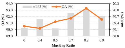
Masking ratio. We further validate the impact of different masking ratios on downstream tasks and separately report the results for classification on ScanObjectNN and semantic segmentation on S3DIS. As shown in Fig. 4, encoding all point patches without masking harms the model’s learning. By employing masking, the overall difficulty of the self-supervised proxy task is increased, thereby aiding the backbone in learning more rich geometric priors. Additionally, our method achieves the best classification and semantic segmentation performance when the mask ratio is 0.8.
5 Conclusion
In conclusion, we propose a novel framework for point cloud pre-training based on diffusion models, called PointDif. It enables the backbone to learn hierarchical geometric prior through the progressive guidance characteristic of the conditional diffusion model. Specifically, we present a conditional point generator to assist the network in learning the point density distribution of the object through point-to-point guidance generation. We also introduce a recurrent uniform sampling strategy on time steps to facilitate the balanced supervision during the backbone’s pre-training. Our extensive experiments on various real-world indoor and outdoor datasets demonstrate significant performance improvements compared to existing methods. Moreover, our proposed method consistently increases performance on competitive backbones. Overall, our diffusion-based pre-training framework provides a new direction for advancing point cloud processing.
References
- Afham et al. [2022] Mohamed Afham, Isuru Dissanayake, Dinithi Dissanayake, Amaya Dharmasiri, Kanchana Thilakarathna, and Ranga Rodrigo. Crosspoint: Self-supervised cross-modal contrastive learning for 3d point cloud understanding. In Proceedings of the IEEE/CVF Conference on Computer Vision and Pattern Recognition, pages 9902–9912, 2022.
- Amit et al. [2021] Tomer Amit, Eliya Nachmani, Tal Shaharbany, and Lior Wolf. Segdiff: Image segmentation with diffusion probabilistic models. arXiv preprint arXiv:2112.00390, 2021.
- Armeni et al. [2016] Iro Armeni, Ozan Sener, Amir R Zamir, Helen Jiang, Ioannis Brilakis, Martin Fischer, and Silvio Savarese. 3d semantic parsing of large-scale indoor spaces. In Proceedings of the IEEE conference on computer vision and pattern recognition, pages 1534–1543, 2016.
- Baranchuk et al. [2021] Dmitry Baranchuk, Ivan Rubachev, Andrey Voynov, Valentin Khrulkov, and Artem Babenko. Label-efficient semantic segmentation with diffusion models. arXiv preprint arXiv:2112.03126, 2021.
- Behley et al. [2019] Jens Behley, Martin Garbade, Andres Milioto, Jan Quenzel, Sven Behnke, Cyrill Stachniss, and Jurgen Gall. Semantickitti: A dataset for semantic scene understanding of lidar sequences. In Proceedings of the IEEE/CVF international conference on computer vision, pages 9297–9307, 2019.
- Chang et al. [2015] Angel X Chang, Thomas Funkhouser, Leonidas Guibas, Pat Hanrahan, Qixing Huang, Zimo Li, Silvio Savarese, Manolis Savva, Shuran Song, Hao Su, et al. Shapenet: An information-rich 3d model repository. arXiv preprint arXiv:1512.03012, 2015.
- Chen et al. [2022] Shoufa Chen, Peize Sun, Yibing Song, and Ping Luo. Diffusiondet: Diffusion model for object detection. arXiv preprint arXiv:2211.09788, 2022.
- Choy et al. [2019] Christopher Choy, JunYoung Gwak, and Silvio Savarese. 4d spatio-temporal convnets: Minkowski convolutional neural networks. In Proceedings of the IEEE/CVF conference on computer vision and pattern recognition, pages 3075–3084, 2019.
- Dai et al. [2017] Angela Dai, Angel X Chang, Manolis Savva, Maciej Halber, Thomas Funkhouser, and Matthias Nießner. Scannet: Richly-annotated 3d reconstructions of indoor scenes. In Proceedings of the IEEE conference on computer vision and pattern recognition, pages 5828–5839, 2017.
- Devlin et al. [2018] Jacob Devlin, Ming-Wei Chang, Kenton Lee, and Kristina Toutanova. Bert: Pre-training of deep bidirectional transformers for language understanding. arXiv preprint arXiv:1810.04805, 2018.
- Dhariwal and Nichol [2021] Prafulla Dhariwal and Alexander Nichol. Diffusion models beat gans on image synthesis. Advances in neural information processing systems, 34:8780–8794, 2021.
- Guo et al. [2023] Ziyu Guo, Xianzhi Li, and Pheng Ann Heng. Joint-mae: 2d-3d joint masked autoencoders for 3d point cloud pre-training. arXiv preprint arXiv:2302.14007, 2023.
- He et al. [2022] Kaiming He, Xinlei Chen, Saining Xie, Yanghao Li, Piotr Dollár, and Ross Girshick. Masked autoencoders are scalable vision learners. In Proceedings of the IEEE/CVF Conference on Computer Vision and Pattern Recognition, pages 16000–16009, 2022.
- Ho et al. [2020] Jonathan Ho, Ajay Jain, and Pieter Abbeel. Denoising diffusion probabilistic models. Advances in Neural Information Processing Systems, 33:6840–6851, 2020.
- Huang et al. [2023a] Di Huang, Sida Peng, Tong He, Honghui Yang, Xiaowei Zhou, and Wanli Ouyang. Ponder: Point cloud pre-training via neural rendering. In Proceedings of the IEEE/CVF International Conference on Computer Vision, pages 16089–16098, 2023a.
- Huang et al. [2021] Siyuan Huang, Yichen Xie, Song-Chun Zhu, and Yixin Zhu. Spatio-temporal self-supervised representation learning for 3d point clouds. In Proceedings of the IEEE/CVF International Conference on Computer Vision, pages 6535–6545, 2021.
- Huang et al. [2023b] Tianyu Huang, Bowen Dong, Yunhan Yang, Xiaoshui Huang, Rynson WH Lau, Wanli Ouyang, and Wangmeng Zuo. Clip2point: Transfer clip to point cloud classification with image-depth pre-training. In Proceedings of the IEEE/CVF International Conference on Computer Vision, pages 22157–22167, 2023b.
- Huang et al. [2022] Xiaoshui Huang, Sheng Li, Wentao Qu, Tong He, Yifan Zuo, and Wanli Ouyang. Frozen clip model is efficient point cloud backbone. arXiv preprint arXiv:2212.04098, 2022.
- Kirillov et al. [2023] Alexander Kirillov, Eric Mintun, Nikhila Ravi, Hanzi Mao, Chloe Rolland, Laura Gustafson, Tete Xiao, Spencer Whitehead, Alexander C Berg, Wan-Yen Lo, et al. Segment anything. arXiv preprint arXiv:2304.02643, 2023.
- Lei et al. [2020] Huan Lei, Naveed Akhtar, and Ajmal Mian. Seggcn: Efficient 3d point cloud segmentation with fuzzy spherical kernel. In Proceedings of the IEEE/CVF conference on computer vision and pattern recognition, pages 11611–11620, 2020.
- Li et al. [2023] Junnan Li, Dongxu Li, Silvio Savarese, and Steven Hoi. Blip-2: Bootstrapping language-image pre-training with frozen image encoders and large language models. arXiv preprint arXiv:2301.12597, 2023.
- Li et al. [2018] Yangyan Li, Rui Bu, Mingchao Sun, Wei Wu, Xinhan Di, and Baoquan Chen. Pointcnn: Convolution on x-transformed points. Advances in neural information processing systems, 31, 2018.
- Lin et al. [2023] Chen-Hsuan Lin, Jun Gao, Luming Tang, Towaki Takikawa, Xiaohui Zeng, Xun Huang, Karsten Kreis, Sanja Fidler, Ming-Yu Liu, and Tsung-Yi Lin. Magic3d: High-resolution text-to-3d content creation. In Proceedings of the IEEE/CVF Conference on Computer Vision and Pattern Recognition, pages 300–309, 2023.
- Liu et al. [2022] Haotian Liu, Mu Cai, and Yong Jae Lee. Masked discrimination for self-supervised learning on point clouds. In Computer Vision–ECCV 2022: 17th European Conference, Tel Aviv, Israel, October 23–27, 2022, Proceedings, Part II, pages 657–675. Springer, 2022.
- Liu et al. [2023] Minghua Liu, Chao Xu, Haian Jin, Linghao Chen, Mukund Varma T, Zexiang Xu, and Hao Su. One-2-3-45: Any single image to 3d mesh in 45 seconds without per-shape optimization, 2023.
- Lu et al. [2022a] Cheng Lu, Yuhao Zhou, Fan Bao, Jianfei Chen, Chongxuan Li, and Jun Zhu. Dpm-solver: A fast ode solver for diffusion probabilistic model sampling in around 10 steps. arXiv preprint arXiv:2206.00927, 2022a.
- Lu et al. [2022b] Cheng Lu, Yuhao Zhou, Fan Bao, Jianfei Chen, Chongxuan Li, and Jun Zhu. Dpm-solver++: Fast solver for guided sampling of diffusion probabilistic models. arXiv preprint arXiv:2211.01095, 2022b.
- Luo and Hu [2021] Shitong Luo and Wei Hu. Diffusion probabilistic models for 3d point cloud generation. In Proceedings of the IEEE/CVF Conference on Computer Vision and Pattern Recognition, pages 2837–2845, 2021.
- Misra et al. [2021] Ishan Misra, Rohit Girdhar, and Armand Joulin. An end-to-end transformer model for 3d object detection. In Proceedings of the IEEE/CVF International Conference on Computer Vision, pages 2906–2917, 2021.
- Nichol et al. [2021] Alex Nichol, Prafulla Dhariwal, Aditya Ramesh, Pranav Shyam, Pamela Mishkin, Bob McGrew, Ilya Sutskever, and Mark Chen. Glide: Towards photorealistic image generation and editing with text-guided diffusion models. arXiv preprint arXiv:2112.10741, 2021.
- Pang et al. [2022] Yatian Pang, Wenxiao Wang, Francis EH Tay, Wei Liu, Yonghong Tian, and Li Yuan. Masked autoencoders for point cloud self-supervised learning. In Computer Vision–ECCV 2022: 17th European Conference, Tel Aviv, Israel, October 23–27, 2022, Proceedings, Part II, pages 604–621. Springer, 2022.
- Qi et al. [2017a] Charles R Qi, Hao Su, Kaichun Mo, and Leonidas J Guibas. Pointnet: Deep learning on point sets for 3d classification and segmentation. In Proceedings of the IEEE conference on computer vision and pattern recognition, pages 652–660, 2017a.
- Qi et al. [2017b] Charles Ruizhongtai Qi, Li Yi, Hao Su, and Leonidas J Guibas. Pointnet++: Deep hierarchical feature learning on point sets in a metric space. Advances in neural information processing systems, 30, 2017b.
- Qi et al. [2019] Charles R Qi, Or Litany, Kaiming He, and Leonidas J Guibas. Deep hough voting for 3d object detection in point clouds. In proceedings of the IEEE/CVF International Conference on Computer Vision, pages 9277–9286, 2019.
- Qian et al. [2022a] Guocheng Qian, Yuchen Li, Houwen Peng, Jinjie Mai, Hasan Hammoud, Mohamed Elhoseiny, and Bernard Ghanem. Pointnext: Revisiting pointnet++ with improved training and scaling strategies. Advances in Neural Information Processing Systems, 35:23192–23204, 2022a.
- Qian et al. [2022b] Guocheng Qian, Xingdi Zhang, Abdullah Hamdi, and Bernard Ghanem. Pix4point: Image pretrained transformers for 3d point cloud understanding. arXiv preprint arXiv:2208.12259, 2022b.
- Ramesh et al. [2022] Aditya Ramesh, Prafulla Dhariwal, Alex Nichol, Casey Chu, and Mark Chen. Hierarchical text-conditional image generation with clip latents. arXiv preprint arXiv:2204.06125, 2022.
- Rombach et al. [2022] Robin Rombach, Andreas Blattmann, Dominik Lorenz, Patrick Esser, and Björn Ommer. High-resolution image synthesis with latent diffusion models. In Proceedings of the IEEE/CVF conference on computer vision and pattern recognition, pages 10684–10695, 2022.
- Saharia et al. [2022] Chitwan Saharia, William Chan, Saurabh Saxena, Lala Li, Jay Whang, Emily L Denton, Kamyar Ghasemipour, Raphael Gontijo Lopes, Burcu Karagol Ayan, Tim Salimans, et al. Photorealistic text-to-image diffusion models with deep language understanding. Advances in Neural Information Processing Systems, 35:36479–36494, 2022.
- Song et al. [2020] Jiaming Song, Chenlin Meng, and Stefano Ermon. Denoising diffusion implicit models. arXiv preprint arXiv:2010.02502, 2020.
- Takagi and Nishimoto [2022] Yu Takagi and Shinji Nishimoto. High-resolution image reconstruction with latent diffusion models from human brain activity. bioRxiv, pages 2022–11, 2022.
- Tang et al. [2020] Haotian Tang, Zhijian Liu, Shengyu Zhao, Yujun Lin, Ji Lin, Hanrui Wang, and Song Han. Searching efficient 3d architectures with sparse point-voxel convolution. In Computer Vision–ECCV 2020: 16th European Conference, Glasgow, UK, August 23–28, 2020, Proceedings, Part XXVIII, pages 685–702. Springer, 2020.
- Tang et al. [2023] Junshu Tang, Tengfei Wang, Bo Zhang, Ting Zhang, Ran Yi, Lizhuang Ma, and Dong Chen. Make-it-3d: High-fidelity 3d creation from a single image with diffusion prior. In Proceedings of the IEEE/CVF International Conference on Computer Vision (ICCV), pages 22819–22829, 2023.
- Thomas et al. [2019] Hugues Thomas, Charles R Qi, Jean-Emmanuel Deschaud, Beatriz Marcotegui, François Goulette, and Leonidas J Guibas. Kpconv: Flexible and deformable convolution for point clouds. In Proceedings of the IEEE/CVF international conference on computer vision, pages 6411–6420, 2019.
- Uy et al. [2019] Mikaela Angelina Uy, Quang-Hieu Pham, Binh-Son Hua, Thanh Nguyen, and Sai-Kit Yeung. Revisiting point cloud classification: A new benchmark dataset and classification model on real-world data. In Proceedings of the IEEE/CVF international conference on computer vision, pages 1588–1597, 2019.
- Wang et al. [2022] Haiyang Wang, Shaocong Dong, Shaoshuai Shi, Aoxue Li, Jianan Li, Zhenguo Li, Liwei Wang, et al. Cagroup3d: Class-aware grouping for 3d object detection on point clouds. Advances in Neural Information Processing Systems, 35:29975–29988, 2022.
- Wang et al. [2019] Yue Wang, Yongbin Sun, Ziwei Liu, Sanjay E Sarma, Michael M Bronstein, and Justin M Solomon. Dynamic graph cnn for learning on point clouds. Acm Transactions On Graphics (tog), 38(5):1–12, 2019.
- Wang et al. [2023a] Zhengyi Wang, Cheng Lu, Yikai Wang, Fan Bao, Chongxuan Li, Hang Su, and Jun Zhu. Prolificdreamer: High-fidelity and diverse text-to-3d generation with variational score distillation. arXiv preprint arXiv:2305.16213, 2023a.
- Wang et al. [2023b] Ziyi Wang, Xumin Yu, Yongming Rao, Jie Zhou, and Jiwen Lu. Take-a-photo: 3d-to-2d generative pre-training of point cloud models. In Proceedings of the IEEE/CVF International Conference on Computer Vision, pages 5640–5650, 2023b.
- Wei et al. [2023] Chen Wei, Karttikeya Mangalam, Po-Yao Huang, Yanghao Li, Haoqi Fan, Hu Xu, Huiyu Wang, Cihang Xie, Alan Yuille, and Christoph Feichtenhofer. Diffusion models as masked autoencoders. arXiv preprint arXiv:2304.03283, 2023.
- Wolleb et al. [2022] Julia Wolleb, Robin Sandkühler, Florentin Bieder, Philippe Valmaggia, and Philippe C Cattin. Diffusion models for implicit image segmentation ensembles. In International Conference on Medical Imaging with Deep Learning, pages 1336–1348. PMLR, 2022.
- Woo et al. [2023] Sungmin Woo, Dogyoon Lee, Sangwon Hwang, Woo Jin Kim, and Sangyoun Lee. Mkconv: Multidimensional feature representation for point cloud analysis. Pattern Recognition, 143:109800, 2023.
- Wu et al. [2023a] Chenfei Wu, Shengming Yin, Weizhen Qi, Xiaodong Wang, Zecheng Tang, and Nan Duan. Visual chatgpt: Talking, drawing and editing with visual foundation models. arXiv preprint arXiv:2303.04671, 2023a.
- Wu et al. [2023b] Xiaoyang Wu, Xin Wen, Xihui Liu, and Hengshuang Zhao. Masked scene contrast: A scalable framework for unsupervised 3d representation learning. In Proceedings of the IEEE/CVF Conference on Computer Vision and Pattern Recognition, pages 9415–9424, 2023b.
- Xie et al. [2020] Saining Xie, Jiatao Gu, Demi Guo, Charles R Qi, Leonidas Guibas, and Or Litany. Pointcontrast: Unsupervised pre-training for 3d point cloud understanding. In Computer Vision–ECCV 2020: 16th European Conference, Glasgow, UK, August 23–28, 2020, Proceedings, Part III 16, pages 574–591. Springer, 2020.
- Xu et al. [2021] Jianyun Xu, Ruixiang Zhang, Jian Dou, Yushi Zhu, Jie Sun, and Shiliang Pu. Rpvnet: A deep and efficient range-point-voxel fusion network for lidar point cloud segmentation. In Proceedings of the IEEE/CVF International Conference on Computer Vision, pages 16024–16033, 2021.
- Xu et al. [2023] Jiale Xu, Xintao Wang, Weihao Cheng, Yan-Pei Cao, Ying Shan, Xiaohu Qie, and Shenghua Gao. Dream3d: Zero-shot text-to-3d synthesis using 3d shape prior and text-to-image diffusion models. In Proceedings of the IEEE/CVF Conference on Computer Vision and Pattern Recognition, pages 20908–20918, 2023.
- Yu et al. [2022] Xumin Yu, Lulu Tang, Yongming Rao, Tiejun Huang, Jie Zhou, and Jiwen Lu. Point-bert: Pre-training 3d point cloud transformers with masked point modeling. In Proceedings of the IEEE/CVF Conference on Computer Vision and Pattern Recognition, pages 19313–19322, 2022.
- Zeng et al. [2023] Yihan Zeng, Chenhan Jiang, Jiageng Mao, Jianhua Han, Chaoqiang Ye, Qingqiu Huang, Dit-Yan Yeung, Zhen Yang, Xiaodan Liang, and Hang Xu. Clip2: Contrastive language-image-point pretraining from real-world point cloud data. In Proceedings of the IEEE/CVF Conference on Computer Vision and Pattern Recognition, pages 15244–15253, 2023.
- Zhang et al. [2022] Renrui Zhang, Ziyu Guo, Peng Gao, Rongyao Fang, Bin Zhao, Dong Wang, Yu Qiao, and Hongsheng Li. Point-m2ae: multi-scale masked autoencoders for hierarchical point cloud pre-training. arXiv preprint arXiv:2205.14401, 2022.
- Zhang et al. [2021] Zaiwei Zhang, Rohit Girdhar, Armand Joulin, and Ishan Misra. Self-supervised pretraining of 3d features on any point-cloud. In Proceedings of the IEEE/CVF International Conference on Computer Vision, pages 10252–10263, 2021.
- Zhao et al. [2023] Shihao Zhao, Dongdong Chen, Yen-Chun Chen, Jianmin Bao, Shaozhe Hao, Lu Yuan, and Kwan-Yee K Wong. Uni-controlnet: All-in-one control to text-to-image diffusion models. arXiv preprint arXiv:2305.16322, 2023.
- Zhu et al. [2021] Xinge Zhu, Hui Zhou, Tai Wang, Fangzhou Hong, Yuexin Ma, Wei Li, Hongsheng Li, and Dahua Lin. Cylindrical and asymmetrical 3d convolution networks for lidar segmentation. In Proceedings of the IEEE/CVF conference on computer vision and pattern recognition, pages 9939–9948, 2021.
Supplementary Material
6 Proof
Calculating the probability distribution for the reverse process is hard. However, given , the posterior of the forward diffusion process can be calculated using the following equation:
| (16) |
| (17) |
According to Eq. 6 in the main text, the variational lower bound can be divided into three parts:
| (18) |
is a constant without parameters and can be ignored. To compute the parameterization of , following [14], we set the mean of to:
| (19) |
We can calculate :
| (20) |
where is a parameter-free constant that can be disregarded. By substituting Eq. 17 and Eq. 19 into :
| (21) |
where is a constant that is unrelated to the loss, and following [14], we can further simplify the training loss:
| (22) |
7 Implementation Details
All experiments are conducted on the RTX 3090 GPU. We describe the details of fine-tuning on various tasks.
Object classification. We use a three-layer MLP with dropout as the classification head. During the fine-tuning process, we sample 2048 points for each point cloud, divide them into 128 point patches, set the learning rate to 5e-4, and fine-tune for 300 epochs.
3D object detection. Unlike MaskPoint [24], which is pre-trained on ScanNet-Medium and loads the weights of both the SA layer and the encoder during fine-tuning. During the fine-tuning stage, we only load the weights of the transformer encoder pre-trained on ShapeNet [6]. Following Maskpoint, we set the learning rate to 5e-4 and use the AdamW optimizer with a weight decay of 0.1. The batch size is set to 8.
| Methods |
mIoU |
car |
bicycle |
motorcycle |
truck |
other-vehicle |
person |
bicyclist |
motorcyclist |
road |
parking |
sidewalk |
other-ground |
building |
fence |
vegetation |
trunk |
terrain |
pole |
traffic-sign |
|---|---|---|---|---|---|---|---|---|---|---|---|---|---|---|---|---|---|---|---|---|
| Cylinder3D [63] | 66.1 | 96.9 | 54.4 | 75.9 | 81.0 | 67.0 | 79.3 | 92.4 | 0.1 | 94.6 | 47.9 | 82.2 | 0.1 | 90.3 | 57.0 | 85.9 | 66.9 | 69.2 | 63.6 | 50.6 |
| SPVCNN [42] | 68.5 | 97.9 | 59.8 | 81.1 | 79.8 | 80.8 | 80.0 | 92.0 | 0.6 | 94.2 | 50.4 | 81.7 | 0.6 | 90.9 | 63.5 | 88.0 | 69.7 | 74.1 | 65.8 | 51.5 |
| RPVNet [56] | 68.9 | 97.9 | 42.8 | 87.6 | 91.2 | 83.5 | 78.3 | 90.2 | 0.7 | 95.2 | 57.1 | 83.1 | 0.2 | 91.0 | 63.2 | 87.3 | 71.4 | 72.0 | 64.9 | 51.5 |
| MinkowskiNet [8] | 70.2 | 97.4 | 56.1 | 84.9 | 84.0 | 79.1 | 81.9 | 91.4 | 24.0 | 94.0 | 52.2 | 81.3 | 0.2 | 92.0 | 67.2 | 88.4 | 68.6 | 74.8 | 65.5 | 50.6 |
| MinkowskiNet+PointDif | 71.3 | 97.5 | 58.8 | 84.6 | 92.8 | 80.6 | 81.4 | 92.3 | 30.3 | 94.1 | 56.0 | 81.7 | 0.2 | 91.4 | 65.4 | 88.5 | 69.1 | 75.2 | 65.0 | 50.5 |
| Methods |
Metric |
Overall |
cabinet |
bed |
chair |
sofa |
table |
door |
window |
bookshelf |
picture |
counter |
desk |
curtain |
refrigerator |
showercurtrain |
toilet |
sink |
bathtub |
garbagebin |
|---|---|---|---|---|---|---|---|---|---|---|---|---|---|---|---|---|---|---|---|---|
| CAGroup3D [46] | 73.20 | 54.39 | 85.78 | 95.70 | 91.95 | 69.67 | 67.87 | 60.84 | 63.71 | 38.70 | 73.62 | 82.12 | 66.96 | 58.32 | 75.80 | 99.97 | 77.85 | 87.74 | 66.61 | |
| CAGroup3D+PointDif | 74.14 | 53.71 | 87.85 | 95.46 | 89.73 | 73.01 | 69.36 | 59.72 | 65.22 | 41.65 | 75.07 | 82.66 | 67.10 | 56.27 | 79.22 | 99.91 | 82.27 | 89.55 | 66.69 | |
| CAGroup3D [46] | 60.84 | 39.01 | 81.51 | 90.24 | 82.75 | 65.89 | 53.47 | 36.39 | 55.82 | 25.13 | 42.01 | 66.19 | 49.33 | 53.16 | 57.73 | 96.52 | 53.80 | 86.75 | 59.35 | |
| CAGroup3D+PointDif | 61.31 | 38.47 | 82.46 | 91.03 | 82.23 | 67.09 | 53.88 | 34.72 | 56.80 | 31.34 | 40.02 | 65.49 | 48.19 | 51.40 | 70.57 | 96.37 | 52.60 | 82.33 | 58.53 |
Semantic segmentation on indoor dataset. For a fair comparison, we put all pre-trained transformer encoders within the same codebase and freeze them while fine-tuning the decoder and semantic segmentation head. Due to limited computing resources, we set the batch size to 4 during fine-tuning. The remaining settings followed those used for training PointNeXt [35] from scratch in the original paper.
Semantic segmentation on outdoor dataset. During fine-tuning, we load the backbone MinkUNet pre-trained on ShapeNet. And fine-tune the entire network while following the same settings used for training MinkowskiNet [8] from scratch.
3D object detection of CAGroup3D with and without pre-training. We load the weights of the backbone BiResNet, which is pre-trained on ShapeNet using our method. Then, we fine-tune the entire CAGroup3D [46] model using the same settings as those used for training CAGroup3D from scratch. Note that, we utilize the official codebase of CAGroup3D and consider the best-reproduced results as the baseline for comparison.
8 Additional results
Semantic segmentation on outdoor dataset. As shown in Tab. 9, We report the mean IoU(%) and the IoU(%) on SemanticKITTI [5] for all semantic classes for different methods. Our method improves mean IoU and IoU for multiple categories compared to the variant trained from scratch. The experimental results also demonstrate that our method performs well on outdoor datasets.
Object detection results of CAGroup3D with and without pre-training. We report the Overall and different category results at (%) and (%). From Tab. 10, we observe that pre-training with our method leads to better performance than training CAGroup3D from scratch. Therefore, our pre-training framework can be flexibly applied to various backbones to improve performance.
Recurrent uniform sampling. Keeping the number of unique point clouds in a batch constant, we conduct experiments with 2 and 8 intervals divisions. The results are shown in Tab. 11, our strategy of dividing the 4 intervals and uniform sampling time step is optimal.
Masking strategy. We report the experimental results for downstream classification and semantic segmentation tasks with different masking strategies. The strategy of block masking involves masking adjacent point patches. From Tab. 12, we observe that random masking performs better than block masking under the same masking ratio (0.8).
| #Point Clouds | # | Intervals | Effective Batchsize | mIoU | mAcc |
|---|---|---|---|---|---|
| 128 | 2 | 2 | 256 | 69.52 | 75.46 |
| 128 | 4 | 4 | 512 | 70.02 | 77.05 |
| 128 | 8 | 8 | 1024 | 69.49 | 76.50 |
9 Additional Visualization.
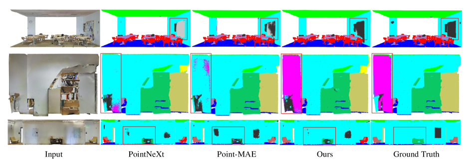
S3DIS semantic segmentation visualizations. We provide a qualitative comparison of results for S3DIS semantic segmentation. As shown in Fig. 5, the predictions of our method are closer to the ground truth and less incorrectly segmented than training PointNeXt from scratch and Point-MAE.
| Masking Strategy | Mask Ratio | OBJ-BG | mIoU |
|---|---|---|---|
| Block | 0.8 | 91.91 | 69.47 |
| Random | 0.8 | 93.29 | 70.02 |
10 limitation
Our pre-training method has demonstrated outstanding performance on various 3D real datasets, but its performance is slightly worse on synthetic datasets. We suspect that this is due to the inability of synthetic datasets to fully simulate the complexity of real-world objects, such as the presence of more noise and occlusion in real datasets. Furthermore, the synthetic datasets are relatively simple, and the performance on the synthetic datasets is currently saturated, with only slight improvements from other pre-training methods. Therefore, it is insufficient to demonstrate the performance advantage of the algorithm on the synthetic datasets. In the future, we will continue exploring and fully exploiting diffusion models’ beneficial impact on point cloud pre-training. We also hope that our work will inspire more research on pre-training with diffusion models, contributing to the advancement of the field.