Polarization Signatures of Relativistic Magnetohydrodynamic Shocks in the Blazar Emission Region - I. Force-free Helical Magnetic Fields
Abstract
The optical radiation and polarization signatures in blazars are known to be highly variable during flaring activities. It is frequently argued that shocks are the main driver of the flaring events. However, the spectral variability modelings generally lack detailed considerations of the self-consistent magnetic field evolution modeling, thus so far the associated optical polarization signatures are poorly understood. We present the first simultaneous modeling of the optical radiation and polarization signatures based on 3D magnetohydrodynamic simulations of relativistic shocks in the blazar emission environment, with the simplest physical assumptions. By comparing the results with observations, we find that shocks in a weakly magnetized environment will largely lead to significant changes in the optical polarization signatures, which are seldom seen in observations. Hence an emission region with relatively strong magnetization is preferred. In such an environment, slow shocks may produce minor flares with either erratic polarization fluctuations or considerable polarization variations, depending on the parameters; fast shocks can produce major flares with smooth PA rotations. In addition, the magnetic fields in both cases are observed to actively revert to the original topology after the shocks. All these features are consistent with observations. Future observations of the radiation and polarization signatures will further constrain the flaring mechanism and the blazar emission environment.
1 Introduction
Blazars are the most violent active galactic nuclei. They are known to emit nonthermal-dominated radiation from radio to -rays with strong variability across the entire electromagnetic spectrum. It is generally agreed that the emission comes from an unresolved region in a relativistic jet that is directed close to our line of sight (LOS). The blazar spectrum has two components. The low-energy component, from radio to optical/UV, is known to be polarized, with the polarization percentage ranging from a few to tens of percent. This is in agreement with the synchrotron emission from nonthermal electrons in a partially ordered magnetic field. Several papers have demonstrated that the observed polarization signatures may indicate a helical magnetic structure (Lyutikov et al., 2005; Pushkarev et al., 2005; Zhang et al., 2015). The high-energy component, from X-rays to -rays, is usually interpreted as originating from inverse Compton scattering by the same nonthermal electrons of soft seed photons (e.g., Marscher & Gear, 1985; Dermer et al., 1992; Sikora et al., 1994), but a hadronic origin cannot be ruled out (e.g., Mannheim & Biermann, 1992; Mücke & Protheroe, 2001; Böttcher et al., 2013). Both spectral components of blazars exhibit fast variability. Many observations show flares in various observational bands lasting days or even hours (e.g., Ciprini, 2011; Chatterjee et al., 2012); in particular, high-energy -rays sometimes show variability time scale within several tens of minutes (e.g., Aharonian et al., 2007; Albert et al., 2007). Based on the causality relation, , where is the Doppler factor and is the observed flaring time scale, the size of the emission region in the comoving frame of the emission region should generally be within . Therefore, it is often argued in the blazar spectral variability fittings that the blazar emission region is a small region near the broad line region of the blazar jet (e.g., Tavecchio et al., 2010; Böttcher et al., 2013; Barnacka et al., 2014).
Blazar spectral fittings have shown that the nonthermal electron spectra responsible for the common blazar SEDs require power-law indices of in most cases (e.g., Böttcher et al., 2013). This is in agreement with numerical simulations of relativistic shocks, which have demonstrated that diffusive shock acceleration forms such power-law spectra (Achterberg et al., 2001; Spitkovsky, 2008; Summerlin & Baring, 2012). Therefore, shocks are frequently used to explain blazar flaring activities. However, in general, numerical simulations of shock acceleration do not provide detailed calculations of the expected radiation features. In terms of the spectral variability fittings, scenarios of relativistic shocks propagating through the jet have been widely investigated (e.g., Marscher & Gear, 1985; Spada et al., 2001; Joshi & Böttcher, 2007; Graff et al., 2008). These models have successfully fit the time-dependent SEDs and multiwavelength light curves of blazar flares, but they usually assume a stationary chaotic magnetic field. Therefore, the polarization variations are poorly understood and/or constrained.
Polarimetry plays an important role in constraining the jet physics. Radio polarimetry has been a standard tool to understand magnetic fields of large-scale jets in radio galaxies (e.g., Laing & Bridle, 2014). Additionally, sometimes blazar flaring activities have been reported to be connected with changes in radio knots (e.g., Marscher et al., 2008). However, since blazar emission regions remain spatially unresolved, high-resolution imaging and polarimetry at radio wavelengths usually cannot directly constrain the physical conditions in the blazar high-energy emission environment. However, the optical emission from the blazar emission region generally dominates over all the other optical emissions from the blazar jet, hence optical polarimetry is able to directly reveal the inner-jet magnetic field structure. The observed optical polarization signatures are generally erratic. Typically, the polarization degree (PD) varies within , but occasionally a higher PD () is reported (e.g., Scarpa & Falomo, 1997). The polarization angle (PA) usually displays perturbations around some mean values. However, polarization signatures can be highly variable during the flaring activities. In particular, significant multiwavelength flaring activities are seen to be accompanied by large () PA rotations (e.g., Marscher et al., 2008; Abdo et al., 2010; Chandra et al., 2015). These flare + PA rotation events often feature smooth PA rotations and apparently time-symmetric light curves and PD patterns. In addition to the individual observations, Blinov et al. (2015) are performing a polarization monitoring program of a large sample, in which they find that blazars with detected PA rotations generally exhibit stronger variations in the PA, and the rotations can go in both directions. Moreover, they claim that the PA rotations are probably physically connected to the -ray flares.
In terms of modeling, several mechanisms have been put forward to understand the polarization signatures, especially the PA rotations. An emission region following a helical trajectory (e.g., Marscher et al., 2008) can give rise to a smooth PA rotation, but such a model prefers all rotations present in the same blazar to follow the same rotating direction, which contradicts observations. An initially chaotic magnetic field structure compressed by a flat shock (Laing, 1980) or multiple small shocks (Marscher, 2014) can produce erratic polarization patterns and occasionally large polarization variations through random walks, but the resulting patterns are normally whimsical, and it has been shown that the observed PA rotations are unlikely to result completely from random walks (Kiehlmann et al., 2013; Blinov et al., 2015). Chen et al. (2014) and Zhang et al. (2014) have proposed a model in which a disturbance propagates through a cylindrical emission region pervaded by a helical magnetic field. This model can give rise to systematic PA rotations and apparently time-symmetric light curves and PD patterns. Based on this model, Zhang et al. (2015) and Chandra et al. (2015) have presented simultaneous fittings of SEDs, light curves and polarization signatures for two flare + PA rotation events. Nonetheless, in all the models mentioned above, the magnetic field evolution is treated in an ad hoc way. Furthermore, none of them can so far explain the statistical properties of the polarization variations as shown in Blinov et al. (2015).
In this paper, we present the first polarization-dependent radiation modeling based on relativistic magnetohydrodynamics (RMHD) simulations of shocks in helical magnetic fields in the blazar emission region. This new approach performs detailed analysis on the interaction between the shock propagation and the magnetic field evolution, which enables us to constrain the blazar emission environment and the shock parameters. We demonstrate that the blazar emission region largely possesses significant magnetic energy. In such an environment, fast shocks can be the driver of flaring events, producing both the typical polarization fluctuations and the occasional large PA rotations. Our simulation results are consistent with the statistical polarization properties reported in Blinov et al. (2015). We will describe our model setup in Section 2, illustrate the interaction between the shock and the magnetic field as well as the consequent radiation and polarization signatures in Section 3, present additional parameter studies in Section 4, and discuss the results in Section 5.
2 Model Setup
The purpose of this paper is to study the time-dependent radiation and polarization signatures resulting from an RMHD shock in the blazar emission environment, with the simplest physical assumptions. In this section, we will describe our physical assumptions and corresponding code structure in detail.
2.1 Physical Assumptions
The blazar emission region is often considered to be an unresolved region near the broad line region of the jet. Generally speaking, the magnetic field topology and evolution as well as plasma flow dynamics in the blazar emission region should be linked with those in the large-scale jet. However, the oberved fast variability and high luminosity suggest that the emission region is an extraordinary, very small and localized region with fast evolution. Therefore, we argue that within the time scale of an individual flare, the blazar emission region can be considered as uncorrelated with the properties of the large-scale jet, even though it is spatially embedded within the jet. On the other hand, the emission region is expected to remain well localized in the jet during flares due to pressure provided by the large-scale jet structure. We assume that flares are due to a disturbance propagating through the emission region. Many observations show that light curves and even the time-dependent polarization signatures appear symmetric in time (e.g., Abdo et al., 2010). This means that the emission region and the disturbance are likely to possess some kind of symmetry. Zhang et al. (2014, 2015) have shown that a helically symmetric emission region and disturbance, with detailed consideration of light-travel-time effects (LTTEs), can naturally explain the apparently time-symmetric light curves and time-dependent polarization signatures. Therefore, we continue to use that assumption here.
Due to the relativistic aberration, even though we are observing blazars nearly along the jet in the observer’s frame (typically, ), where and are the angle between the LOS and the jet direction and the Lorentz factor of the emission region in the observer’s frame, respectively, the angle between LOS and the jet axis in the comoving frame is likely around (if , then ). Zhang et al. (2014) have shown that if the LOS is fixed at some other angles, the general trend of polarization variations is only weakly affected. In addition, as is suggested in the bending jet scenario of the polarization signatures, a change in the LOS direction may significantly affect the polarization signatures. However, those effects are beyond the scope of our first-step study. Thus in all of the following simulations, we choose in the comoving frame, and hence the Doppler factor .
We use ideal RMHD simulations to describe the evolution of the system. The underlying model assumes that a plasma jet is traveling with a Lorentz factor of in the observer’s frame. In the comoving frame of the jet, a flow of plasma which is pervaded by a helical magnetic field travels at a Lorentz factor of . Inside this flow lies a cylindrical emission region containing nonthermal particles. Along the path of the flow it encounters a flat stationary layer of the plasma (the disturbance), forming a shock wave. Thus the total Lorentz factor of the emission region in the observer’s frame is . Although in the following sections our RMHD simulations use different Lorentz factors of the disturbance in the comoving frame of the emission region, of the emission region in the observer’s frame is not constrained. Therefore, we assume a fixed Lorentz factor of for the emission region in the observer’s frame, which is commonly inferred from SED modelings.
Before the emission region interacts with the disturbance, the helical magnetic field is assumed to be in force-balance. The advantage of this magnetic field setup is that it will naturally give rise to comparable poloidal and toroidal contributions, resulting in a relatively low background PD without the need of any turbulence. In addition, this can simplify our setup for the plasma density and the thermal pressure, which are taken to be uniform inside the emission region. In this way, we assume that initially all flow conditions and magnetic fields are laminar, with no preexisting turbulent components. Also, as the RMHD requires an input for the thermal pressure, we assume that in the beginning the plasma is cold and hence the thermal pressure is very small compared to the kinetic energy or the magnetic energy.
In the comoving frame of the emission region, the disturbance and the resulting shock will propagate through the emission region, and change the physical conditions as well as accelerate particles at its location, generating a flare. We apply the simple assumption that the shock will inject fresh nonthermal electrons at the shock front whose energy is equal to a fixed small amount of the local shock kinetic energy. In this way, any deceleration and deformation of the shock due to the magnetic field obstruction can be taken into consideration. In Section 4 we will show that the injection rate does not affect the polarization signatures too much.
We briefly summarize our model assumptions in the following:
1. The emission region is a small cylindrical region embedded in the large-scale jet.
2. The evolution of the emission region is detached from the large-scale jet.
3. The boundary of the emission region is held by a pressure wall, probably provided by the
large-scale jet.
4. In the comoving frame of the emission region, the observer is observing from the side of
the emission region ().
5. The initial magnetic field inside the emission region is a force-free helical magnetic field.
6. Initially all flow conditions and magnetic fields are laminar.
7. Initially the plasma is cold.
8. Initially the disturbance is a flat cylindrical region traveling relativistically in the comoving
frame of the emission region.
9. The disturbance will generate a shock in the emission region. At the shock front, the shock will
inject nonthermal particles whose total energy is a constant, small fraction of the local shock
kinetic energy.
2.2 Code Structure
The above model is realized by the combination of the 3D multi-zone RMHD code LA-COMPASS developed by Li & Li (2003) and the 3D multi-zone polarization-dependent ray-tracing code 3DPol developed by Zhang et al. (2014). Fig. 1 (left) shows a sketch of the simulation setup, and Table 1 presents some major parameters. The RMHD simulation is performed in the comoving frame of the emission region, using Cartesian coordinates. We apply the outflow boundary conditions for the simulation domain; in the following, we will demonstrate that our setup should not suffer from any boundary effects. The simulation domain is pervaded by a helical magnetic field (Fig. 1 (left)). In reality, the poloidal magnetic field lines have to be closed, but based on our assumption the returning magnetic flux is generally outside the simulation domain. The helical magnetic field is assumed to be in force-balance, in the form of
| (1) |
where and are the Bessel functions of the first kind, is the radius, and and are normalization factors of the magnetic field strength and the radius, respectively. The component is assumed to be zero. In order to avoid any boundary effects in , directions and comply with the assumed generally monodirectional , we add an exponential cutoff for both components when approaches zero (). However, the exponential cutoff will lead to a nontrivial magnetic force at the edge of the simulation domain, hence we add a plasma pressure to balance it (Fig. 1 (left)).
| Parameters | Length | Time | Velocity |
|---|---|---|---|
| Relation | |||
| Code Unit | |||
| Physical Value | |||
| Parameters | Magnetic Field | Thermal Pressure | Plasma Density |
| Relation | |||
| Code Unit | |||
| Physical Value |
| Bulk Lorentz factor | |
|---|---|
| Orientation of LOS | |
| Electron minimal energy | |
| Electron maximal energy | |
| Electron power-law index |
The emission region is set to be a fixed volume in the simulation domain ( and ranges from to , see Fig. 2). Since the simulation domain is in the comoving frame of the emission region, the disturbance will travel at a Lorentz factor of in the direction. We assume that the disturbance is a thin layer ( in width) and initially put it at some distance away from the emission region (the disturbance layer ranges from to ) to allow some time for the shock wave to form in the numerical simulation (see Fig. 1 (left) and Fig. 2). In order to avoid boundary effects in direction, we use a sufficiently large range in ( to ), so that at the end of the simulation, no signal has reached the boundary. We define a magnetization factor in the emission region,
| (2) |
where is the electromagnetic energy density, is the specific enthalpy, is the plasma density, is the adiabatic index and is the thermal pressure. We further assume that the plasma is cold. Hence we choose to be a small part () of the electromagnetic energy initially. In this way the magnetization factor is approximately . The relativistic Alfvén speed can then be expressed as
| (3) |
Since the entire simulation domain is axisymmetric, we present a cut in the plane in Fig. 2 to illustrate the initial condition, including the magnetic field and the velocity of the disturbance. Notice that the component is not shown, as in a helical setup, in the plane this component is trivial. Also this figure is for an initial ; for other the velocity appears slightly different. As the RMHD simulation takes Cartesian coordinates, we will transform the results to the cylindrical coordinates and feed into the 3DPol code.
The 3DPol code is focused on the polarization-dependent synchrotron radiation. It uses a cylindrical geometry, and further divides it evenly into multiple zones in , and directions. Each zone has its own magnetic field evolution, which is provided by the RMHD simulations. The nonthermal electrons in each zone are assumed to range between a minimal and a maximal Lorentz factor and , with a fixed spectrum of power-law index of plus an exponential cutoff at the high-energy end,
| (4) |
The nonthermal electron normalization factor is assumed to have two components: a fixed uniform initial background density , and an injected density during the shock. As the electron spectrum is fixed, we will only consider the optical light curves and polarization patterns, which do not suffer from any synchrotron-self absorption and Faraday rotation effects for our parameters. As in the RMHD simulation, all calculations are performed in the comoving frame of the emission region. Given the local magnetic field information and the nonthermal electron population, the 3DPol code will calculate the Stokes parameters at various frequencies at every time step in each zone. Next the code will employ ray-tracing to take account of all LTTEs (see Fig. 1 (right) for an illustration), and add up the incoherent Stokes parameters arriving at the observer at the same time, then Lorentz transform to the observer’s frame so as to obtain the total time-dependent radiation and polarization signatures.
We define the PA in the following way. When the electric vector is parallel to the emission region propagation, (toroidal component dominating). Since the PA has ambiguity, the toroidal dominance happens at , and the poloidal dominance at , where is an integer.
3 Interaction between Shock and Magnetic Field
In this section, we will investigate how the shock speed and the magnetization in the blazar emission environment will affect the time-dependent radiation and polarization signatures. Since we generate the shock by a relativistic disturbance, and the simulation is done in the comoving frame of the emission region, the shock front and its motion can hardly be distinguished from the disturbance. Moreover, as we will see in the following results, during the propagation, both the disturbance and the shock speeds may vary in time. Hence we use the initial Lorentz factor of the disturbance rather than the actual time-dependent shock speed for the parameter study. For the same reason, the magnetization factor in the shock frame will vary in time as well; we choose the initial in the emission region instead. This is also a direct indicator of how much the emission region is magnetized at the beginning. By comparing the results with the general observational features, we will be able to constrain the physics in the emission environment. For this purpose, we will present three cases, namely, , (Case I), , (Case II) and , (Case III). The RMHD simulation results are shown in Figs. 3, 5 and 6 for Case I, II and III, respectively, along with the associated radiation and polarization signatures in Fig. 7. For all the cases studied, we fix the initial nonthermal electron density and the characteristic magnetic field strength . The magnetization factor is adjusted through changing the plasma density. Since we employ a simple electron spectrum, we only study the light curves and polarization patterns in the optical band as examples. Additionally, as the background nonthermal electron density and the injection rate are set as input parameters, we use the relative flux level, where is approximately .
3.1 Effects of Magnetization
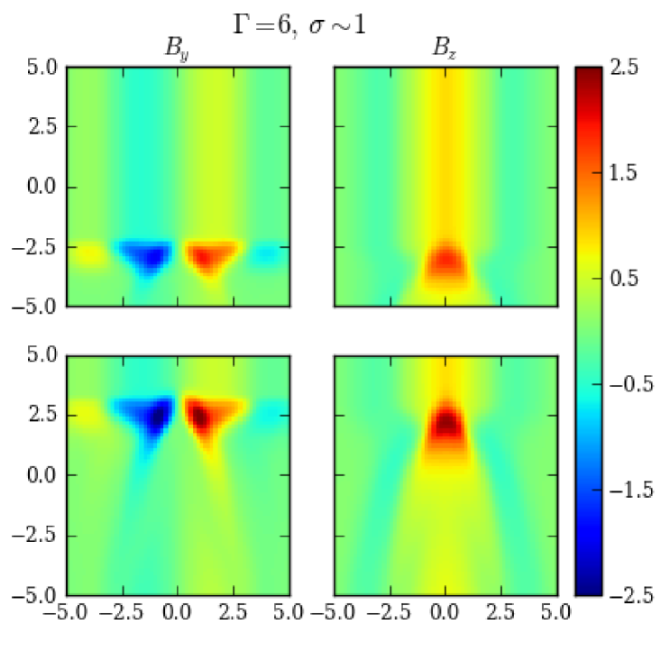
We first examine a kinetic energy dominated environment, Case I. Such an environment is frequently assumed in a shock-initiated flaring model. We first notice that in a trivially magnetized setting (), the speed of Alfvén waves, , is much slower than that of the shock/disturbance. This speed is even slower inside the disturbance. As a result, the entire simulation domain can be treated similar to a hydro setup. Consequently, we can expect that the shock/disturbance will strongly compress the plasma at the shock front, and push it along with the propagation. However, in the ideal MHD, the plasma and the field lines are coupled (frozen-in field lines). Therefore, the toroidal magnetic field lines at the shock front will be greatly compressed, leading to a much larger toroidal contribution; meanwhile, far downstream of the shock, the toroidal lines will be sufficiently stretched, giving rise to a perfectly ordered poloidal magnetic field (see Fig. 3, ). The physical effects described above are the consequence of a shock in a nearly hydro environment with the assumption of the frozen-in field lines. Therefore, we expect that the above shock modifications to the magnetic field structure is not limited to our initial magnetic field topology, but will happen in other magnetic field setups as well. Notice that, however, due to the shock compression, the initial force balance in the radial direction between the magnetic field and plasma pressure and density may be broken. This will lead to some hydrodynamical perturbations in the plasma density and pressure in the radial direction, which are explicitly illustrated in Fig. 4. However, those perturbations are only transported at sonic speeds. This is supported by Fig. 4 where any plasma velocities in the radial direction that arise from those perturbations are non-relativistic. Therefore, although given enough time they may significantly modify the post-shock structures, they are much slower than the time scale that we are interested in in our RMHD simulation. Therefore, we find that those hydrodynamical effects are of minor importance to our current study, and will not discuss them in the following.
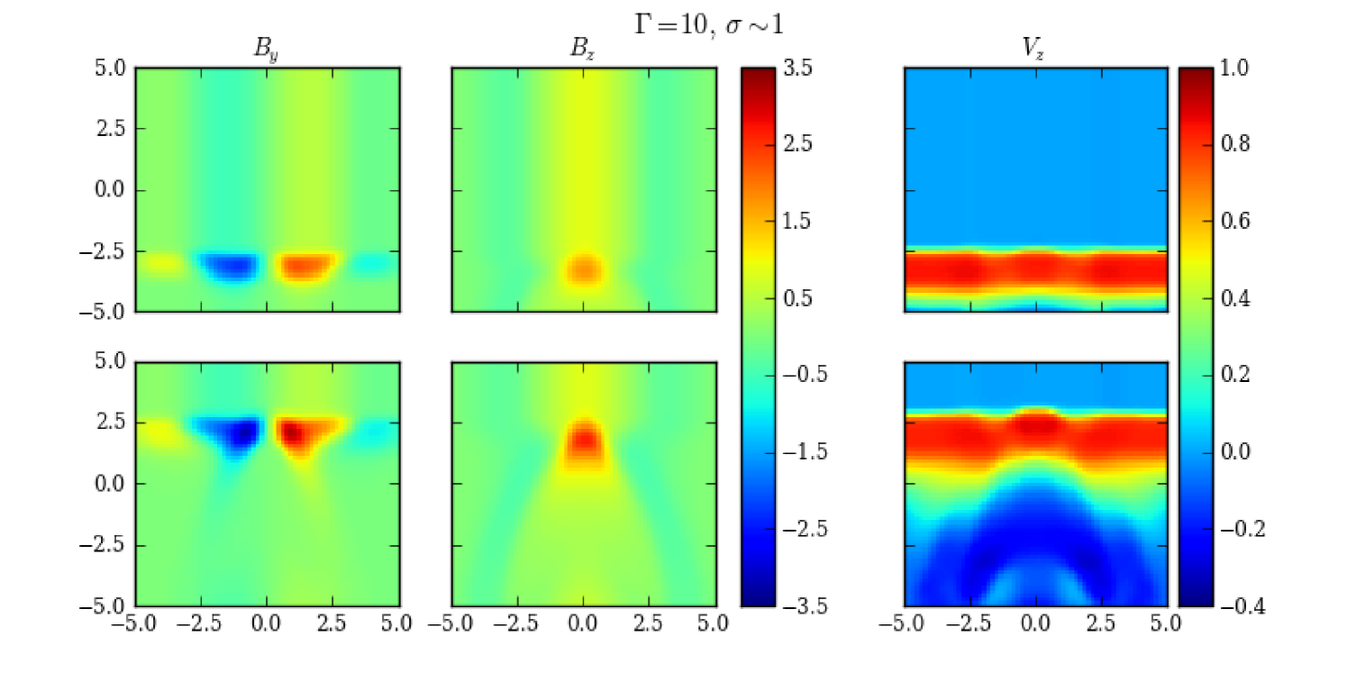
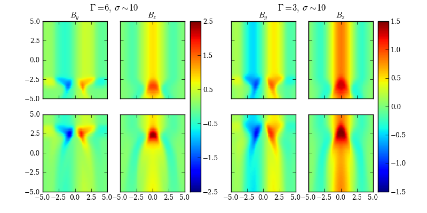
Case II has a moderately magnetized environment (). Hence, the magnetic field will actively participate in the shock propagation. Komissarov & Lyutikov (2011) have calculated that the maximal relativistic shock compression ratio in a magnetized environment is given by
| (5) |
where and are the shock compression ratio and the magnetization factor in the shock frame, respectively. As a result, at the shock front, we can see from the simulation that the shock compression becomes weaker due to the higher magnetization (Fig. 5, ). Furthermore, although initially the emission region has a negligible magnetic force, the enhancement in the toroidal component at the shock front will break down this balance, resulting in a contracting magnetic force in the direction, given by
| (6) |
This contraction is transported by Alfvén waves, which are mildly relativistic in this case. Therefore, in addition to the compression in the direction at the shock front, there exists a contraction of the plasma in the direction. Because of the frozen-in field lines, the poloidal component will be strengthened at the shock front (Fig. 5, ). We can see from the simulation that at a later stage, the increase in the poloidal component gradually gets closer to that in the toroidal component, and even the shape of the shock/disturbance is modified, showing a bullet shape at the central part (Fig. 5 ). Moreover, at variance with Case I, far downstream of the shock/disturbance, even though some plasma is pushed away by the shock/disturbance, the magnetic field is observed acting to revert to its initial topology (Fig. 5, and ).
In the spectral variability fitting, it is frequently argued that during the shock propagation, the local magnetic field either generally maintains its strength and topology (Sokolov et al., 2004; Joshi & Böttcher, 2007), or reverts to its initial state after the shock (Chen et al., 2014; Zhang et al., 2014). This requirement is often necessary to produce the best fittings. Our simulations demonstrate that this can only happen in an adequately magnetized emission region. Therefore, detailed analysis of the magnetic field evolution and shock dynamics should play an essential part in those spectral variability models.
We notice that in both simulations, there are regions with negative (Figs. 3 and 5, ). This is likely due to the reverse shock. In reality, the reverse shock may also lead to some radiation and polarization signatures, but its effect is expected to be weaker than the main shock. Thus in the following we will not consider it.
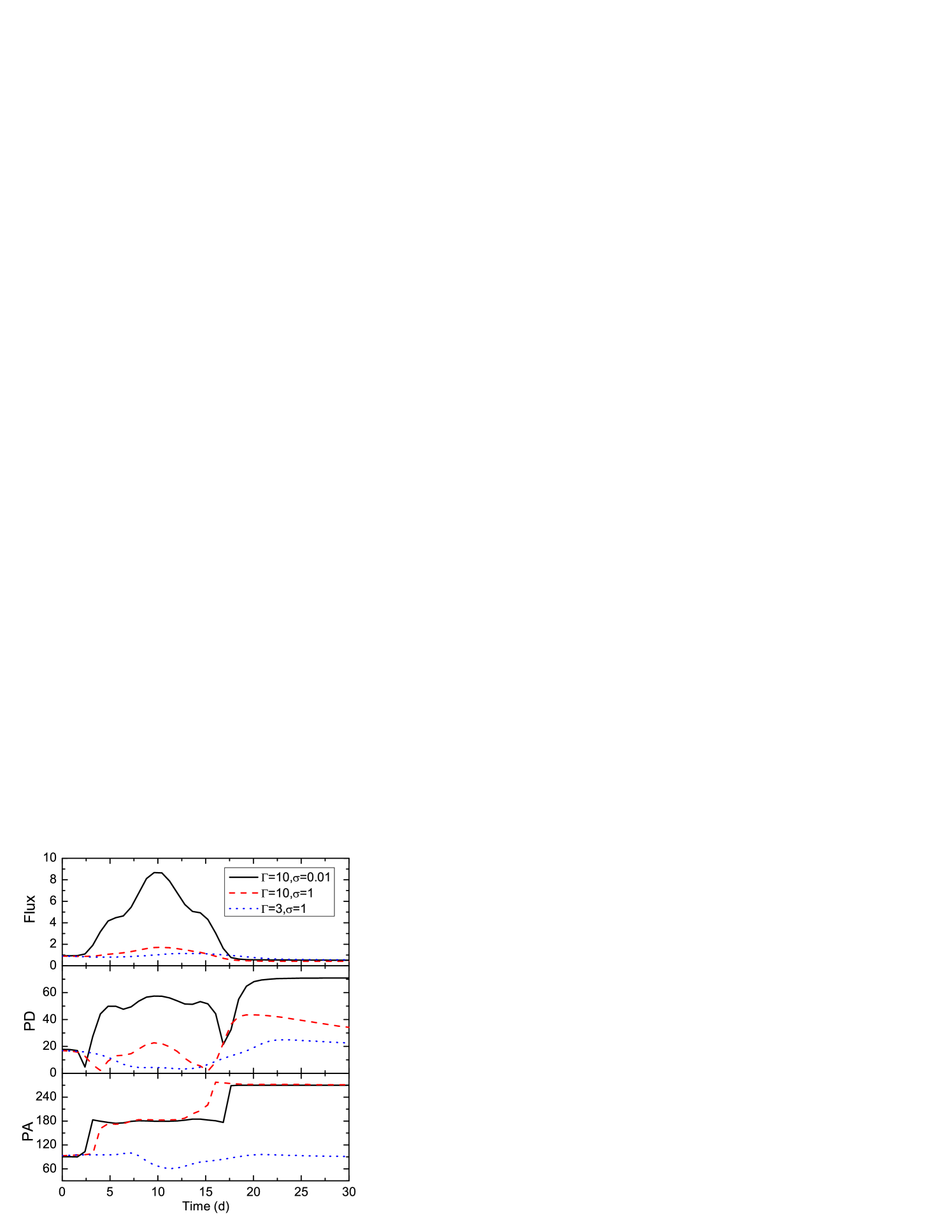
Now we will consider the radiation and polarization signatures resulting from the above RMHD simulations, calculated using the 3DPol code. The general trends are similar for both cases. Before the shock moves in, the entire emission region is axisymmetric. Although the poloidal and toroidal components are comparable in the force-free setup, due to the LOS effect, the projected toroidal component onto the plane of sky is weaker than the projected poloidal component. Therefore initially the emission region has a total polarization dominated by the poloidal component (Fig. 7). When the shock moves in, the toroidal component is strongly increased and fresh nonthermal electrons are injected at the shock front. However, due to the LTTEs, only a small elliptical region on the right that is near the observer is seen (the near side, see Fig. 1 (right), red). Therefore, the flux is seen to gradually increase. Nevertheless, since the toroidal enhancement is strong, a small flaring region is adequate to push the polarization to be dominated by the toroidal component. As a result, the PA quickly rotates to and forms a plateau, which corresponds to the toroidal domination. The PD first experiences a drop which indicates a switch in the domination between the two components, then climbs up to a high level, implying a strong toroidal dominance (Fig. 7). When the shock is about to leave the emission region, the flaring region reaches maximum (Fig. 1 (right), green). Hence the flux peaks. After that, the flaring region moves far from the observer to the left (the far side, Fig. 1 (right), blue), so the flux gradually decreases in an apparently symmetric pattern. However, as some plasma and the coupled magnetic field lines have been pushed away by the shock/disturbance, the total magnetic field strength is smaller than the initial state. Hence the flux level is lower than the initial value. For the same reason, the toroidal contribution is weakened near the end of the flare, hence the PD rises up higher than the initial value, revealing a stronger poloidal contribution. Since the helical magnetic field direction on the far side is opposite to that on the near side, the PA instead completes a rotation to the initial value ( PA ambiguity, Fig. 7).
The major differences between Case I and II are the following. First, due to the stronger magnetic field, Case II has a weaker compression in the toroidal component at the shock front than Case I, while it experiences a rise in the poloidal contribution. Therefore, the PA rotation in Case II appears smoother and has a shorter toroidal dominated plateau than Case I. Also the maximal flare level in Case II is lower. More importantly, near the end of the flare, the moderate magnetization in Case II is acting to restore the initial magnetic topology, hence even if the PD rises above the initial value, it immediately starts to decrease, indicating the recovery of the toroidal component (Fig. 7). Abdo et al. (2010) have shown that at the end of a flare + PA swing event in 3C 279, the PD rises up above the initial value, which is immediately followed by a significant restoration to approximately the initial PD level. The same restoring phases are seen in a number of flare + PA rotation events as well (Larionov et al., 2008; Larionov et al., 2013; Morozova et al., 2014). On the other hand, in Case I the magnetization is too weak, thus the PD rises up to at the end of the flare and shows no restoration, indicating a purely poloidal magnetic structure. As is mentioned above, such a phenomenon is generally the consequence of a trivially magnetized environment, and it is expected to happen with other initial magnetic field topologies. Therefore, we argue that such drastic changes in the polarization signatures are unrealistic compared to observations, so that a nearly unmagnetized emission environment model can be ruled out.
3.2 Effects of Shock Speed
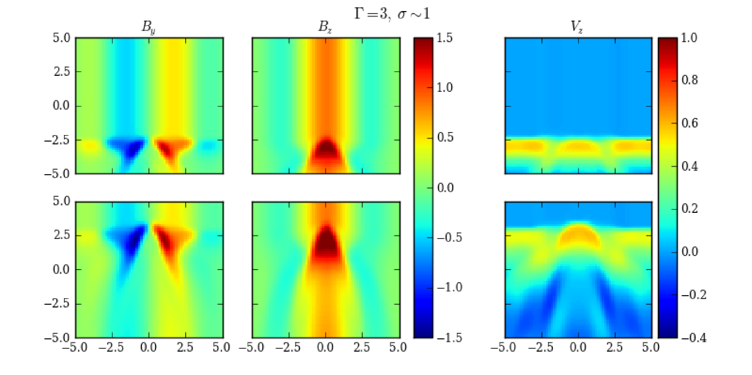
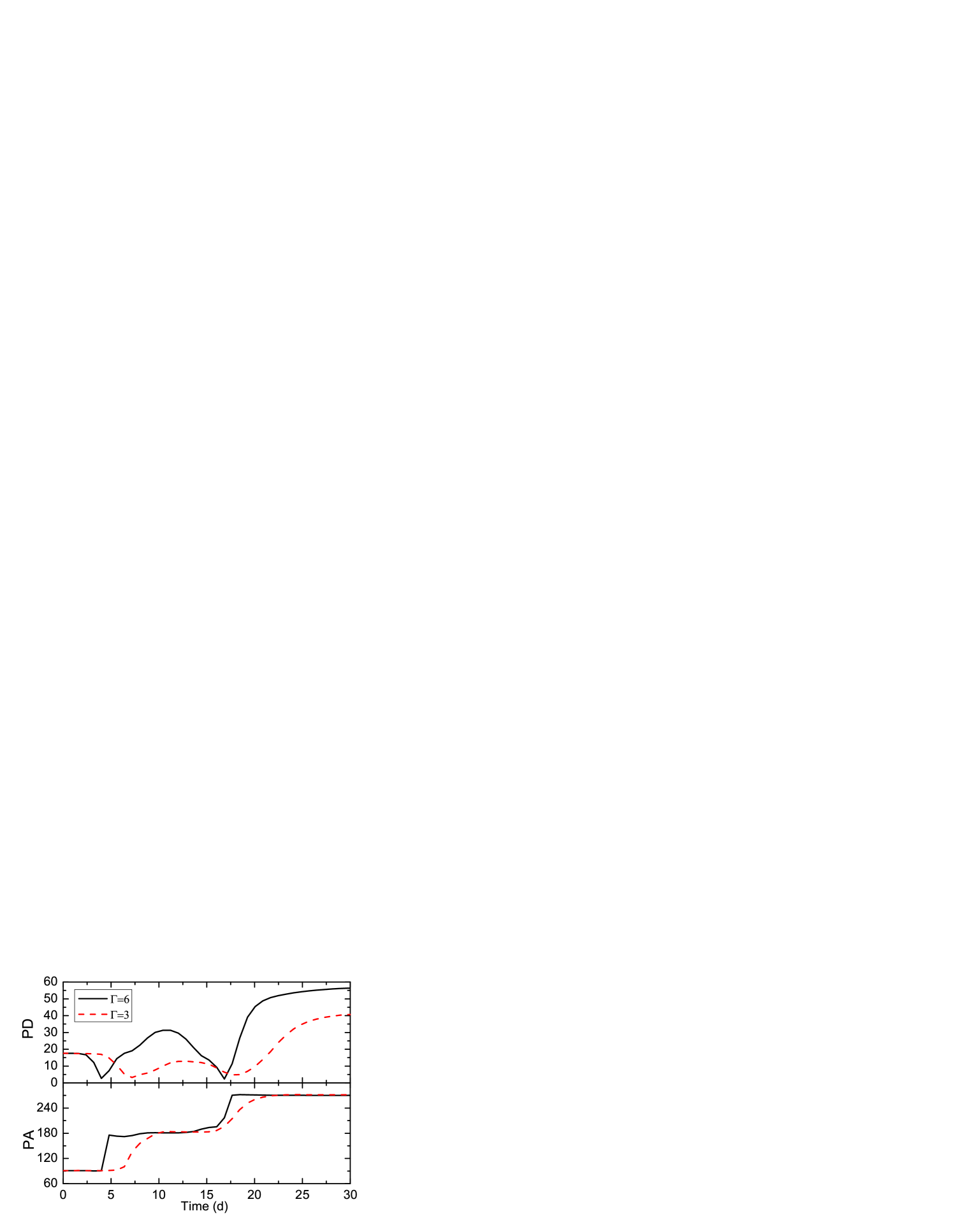
The effects of the shock speed are rather straightforward. We will illustrate those by examining Case III, which shares the same magnetization as Case II but has a slower disturbance. A slower disturbance has less kinetic energy. Therefore, as the shock/disturbance propagates, it cannot exert a very strong pressure onto the plasma; in return the plasma will decelerate the shock/disturbance. Thus we see in Fig. 6 that the shock/disturbance is considerably slower than the initial value (). Therefore, the flare duration is much longer than the previous cases (Fig. 7). Also the shock/disturbance will provide less compression in the plasma at the shock front. As a result, we observe in the simulation that the toroidal component is only moderately increased and stretched at the shock front and downstream of the shock/disturbance, respectively (Fig. 6, ). Moreover, the shower shock/disturbance takes longer time to propagate through the emission region, allowing for further information exchange by Alfvén waves. Therefore, the contraction of the plasma at the shock front, due to the enhanced toroidal component, is seen to catch up with the shock compression. This leads to a considerably strengthened poloidal component at the shock front. Consequently, the PA rotation disappears; instead it shows fluctuations around the initial value. However, at the flare top, the poloidal contribution is only marginally stronger than the toroidal contribution. Therefore, the PD still displays a decrease at the middle of the flare (Fig. 7). Meanwhile, downstream of the shock/disturbance, Alfvén waves restore the initial magnetic field topology to a large extent (Fig. 6, and ). Hence the final PD is not too much higher than the initial value, and gradually recovers after the flare (Fig. 7). Another interesting effect is that due to the weaker kinetic energy in the shock/disturbance and longer influence of Alfvén waves, the shape of the shock/disturbance is distorted (Fig. 6, ). Thus the polarization patterns, especially the PA, appear less symmetric in time than the previous cases (Fig. 7).
4 Parameter Study
In this section, we will perform parameter studies to constrain the shock speed and the magnetization of the emission environment, by comparing the polarization signatures with the general observational properties. Since the injection rate at the shock front is somewhat arbitrary, we will not compare the light curves. Although in principle the injection rate will affect the polarization signatures, in the following we will demonstrate that the polarization signatures are mainly the consequence of the magnetic field evolution. Here we use moderate () and slow () speeds, as well as weak (), strong () and moderate () magnetization factors as examples.
4.1 Weakly Magnetized Environment,
We study a weakly magnetized setup (), with the application of moderate () and slow () disturbances. Due to the small magnetization factor, the mediation by Alfvén waves is slow. Nevertheless, especially in the case of a slow disturbance, the effects of the magnetization cannot be overlooked: the poloidal component is slightly enhanced at the shock front, and the shape of the shock/disturbance is changed (Fig. 8, and ). As a consequence, the polarization patterns appear relatively smooth, in particular the PA rotation (Fig. 9). However, downstream of the shock/disturbance, Alfvén waves fail to restore the initial magnetic topology. Hence at the end of the flare, the PD rises up and maintains a high level (), without showing any restoring phase (Fig. 9). This implies that in a weakly magnetized emission environment, shocks can easily alter the magnetic topology, causing significant changes in the polarization signatures. On the contrary, such polarization variations are seldom reported in observations. Therefore, we do not favor a weakly magnetized emission environment.
4.2 Strongly Magnetized Environment,
Next we consider an emission region with a high magnetization factor (). Here Alfvén waves become relativistic, thus the shock compression is much weaker. All effects of the magnetization as in Case II and III show up. The difference is that even in the case of a medium speed disturbance (), the increase in the poloidal component is higher than that in the toroidal field at the shock front (Fig. 10, and ). Therefore, the PA patterns for both cases exhibit no rotation (Fig. 11). Additionally, the shock/disturbance is greatly distorted. Hence both the PD and the PA patterns appear rather erratic, showing a lot of bumps throughout the flare (Fig. 11), even though the general geometry is rather symmetric. Finally, the restoration downstream of the shock/disturbance is very fast (Fig. 10 and ), thus the PD only rises up gently above the initial value, and quickly recovers at the end of the flare (Fig. 11).
Notice that for a sufficiently fast shock/disturbance, a PA rotation may reappear. However, we expect that such a rotation is likely to be very smooth, without a long toroidal dominated plateau as in Case I to III. Meanwhile the PD variation can be within some small value. This may agree with the observed flare + PA rotation events. To summarize, a strongly magnetized emission environment may generate the typical erratic perturbations in the polarization signatures in the condition of a relatively slow disturbance, together with the smooth flare + PA rotation events provided a relatively fast disturbance. Thus we prefer an emission region with high magnetization.

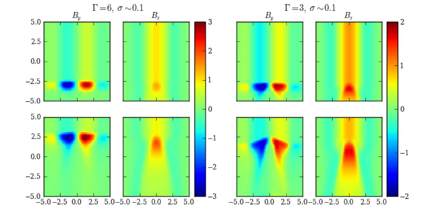
4.3 Transition Point: Moderately Magnetized Environment,
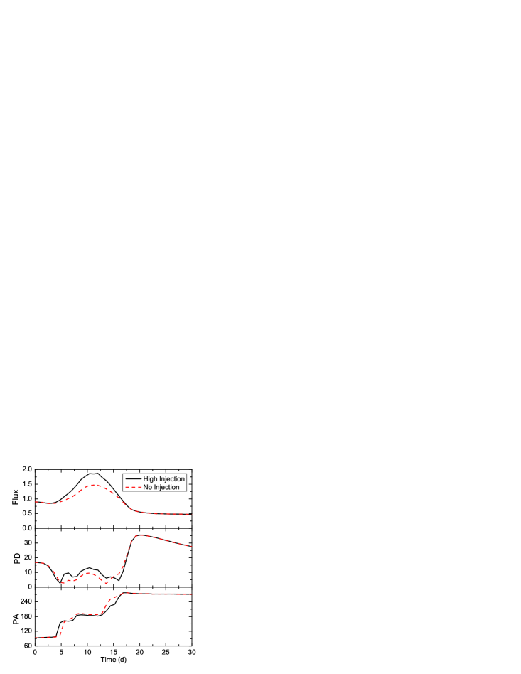
Finally we take a look at an intermediate condition, and . This case shares the same magnetization factor as Case II and III. From the simulation we can see that the general features are similar, but the increases in the poloidal and the toroidal components at the shock front are nearly identical (Fig. 12 (left), and ). However, since the emission region is a cylinder, a larger fraction (at larger radii) of the emission region possesses the enhanced toroidal component. Hence we expect that the radiation during the flare should have more toroidal contributions. In order to test the effects of the injection rate, we perform two 3DPol runs: one with an artificially increased injection rate (approximately ten times higher than the normal value), and one with no injection; the results are shown in Fig. 12 (right). We observe that although the flare level of the high injection case is much higher than the no injection case, the polarization variations appear similar (Fig. 12 (right)). This indicates that the polarization signatures in our calculation are largely due to the magnetic field evolution, instead of the ad hoc nonthermal electron injection rate. We can see that the PA rotation does not show significant toroidal dominated plateau. A number of flare + PA rotation events feature continuous PA rotations without any obvious plateau step (e.g., Marscher et al., 2008; Abdo et al., 2010; Chandra et al., 2015). Based on our simulations, we suggest that such events are likely originating from a sufficiently magnetized environment with a relatively fast disturbance traveling through. Also in this case a vigorous restoring phase is present.
5 Discussions and Summary
We have presented the first polarization-dependent radiation modeling based on RMHD simulations of relativistic shocks in helical magnetic fields in the blazar emission region. We find in Section 3 that the magnetic field evolution during the shock is intrinsically governed by a competition between the shock speed and the magnetization in the emission region: the shock/disturbance tries to alter the magnetic topology, while the magnetization attempts to resist any modifications. We then investigate the parameter space in Section 4 to further constrain the shock parameters and the magnetization in the emission environment. In the following we will summarize the major features and illustrate their connections to observations.
We set up an emission region initially pervaded by a purely helical magnetic field with comparable poloidal and toroidal contributions. Due to the LOS effect, at the beginning the polarization is dominated by the poloidal component. A flat relativistic disturbance, traveling parallel to , will then form a shock wave and propagate through the emission region. In a weakly magnetized environment (), the magnetic field cannot compete against the shock/disturbance. Hence even a mildly relativistic shock/disturbance can permanently change the magnetic topology to a large extent (here ”permanently” means on a time scale that is much longer than the flare duration). This results in drastic variations in the polarization signatures, with no signs of recovery. Such phenomena are hardly detected, thus we conclude that a weakly magnetized emission region is not favored.
In a strongly magnetized emission region (), the magnetic field topology is able to survive the impact of the shock/disturbance. For the slow cases, the shock/disturbance is unable to build up a strong toroidal component, thus the polarization signatures usually exhibit rather erratic fluctuations, which are typical in observations. If the shock/disturbance is slightly faster, then it is plausible to build up the toroidal component and lead to significant polarization variations such as the PA rotations; but in both cases, the flux will not increase sufficiently to produce a flare. Such polarization variations with no obvious flares are consistent with some observations (e.g., Itoh et al., 2013; Jorstad et al., 2013). However, Kirk et al. (2000) and Achterberg et al. (2001) have shown that for relativistic shocks, the hardest obtainable particle power-law index is approximately
| (7) |
where is the power-law index and is the shock compression ratio mentioned previously. We estimate that the strongest shock in our slow disturbance cases can only reach a nonthermal particle spectrum of power-law index of , which is too soft to fit the general blazar SEDs. In addition, relativistic collisionless shocks in the highly magnetized regime may be unable to generate fluctuating magnetic fields and hence inhibit Fermi acceleration (e.g., Sironi et al., 2015). Therefore, a slow shock/disturbance may not efficiently accelerate nonthermal particles that are necessary to generate a flare. This poses a tricky problem for slow shocks. On the other hand, for a relatively fast shock/disturbance, the polarization variations can either fluctuate around some mean value or smoothly rotate in the PA and present a restoring phase at the end of the flare; both are detected in observations (e.g., Larionov et al., 2008; Abdo et al., 2010; Blinov et al., 2015). In summary, we prefer a strongly magnetized emission region, in which fast disturbances can be the driver of the flaring activities.
Observations and spectral variability fittings have shown that the typical Lorentz factor of the blazar emission region is within a few tens (e.g., Jorstad et al., 2005; Böttcher et al., 2013). This is likely to be the upper limit of the shock speed. Therefore, a sufficiently magnetized emission environment will mostly prohibit any dramatic polarization variations, such as the PA rotations and the sudden changes in the PD (flares in the polarized flux). For the blazar emission regions with a weaker magnetization, the PD flares and the PA rotations are triggered by strong shocks. Hence we expect strong nonthermal electron injections. Therefore, intense polarization variations are probably accompanied by vigorous multiwavelength flares. These findings are consistent with observations (Blinov et al., 2015). Another implication is that the blazar emission region presumably maintains a relatively high magnetization, thus it cannot dissipate too much magnetic energy during the shock-initiated flaring activities.
An alternative may weaken some of the constraints mentioned above. In a highly magnetized region, magnetic reconnection can also be the driver of flares. Several authors have illustrated that reconnection can efficiently accelerate nonthermal particles to form a power-law spectrum (Guo et al., 2014; Sironi & Spitkovsky, 2014; Li et al., 2015). In our simulations, no preexisting turbulent magnetic field is present; but in reality, some amount of turbulence may exist. Therefore, during the shock propagation, magnetic reconnection can happen simultaneously, especially in the compression regions at the shock front. This can provide extra nonthermal particles, thus a slow shock in a partially turbulent, partially ordered (such as a helical geometry) magnetic field structure may generate the necessary nonthermal electrons. Several models investigating the reconnection in a highly magnetized environment have been proposed to explain very fast blazar events (Giannios et al., 2009; Deng et al., 2015; Guo et al., 2015). Meanwhile, recent simultaneous fittings of blazar SEDs, light curves and polarization signatures also favor a reconnection process (Zhang et al., 2015; Chandra et al., 2015). During a reconnection event, the magnetic field topology can be greatly modified, which may give rise to some interesting polarization signatures as well. Therefore, we expect that even in a highly magnetized environment, if the reconnection drives the flaring activities, considerable polarization variations are possible. Future observations featuring both the radiation and polarization signatures, along with detailed modelings and simulations of the shock and magnetic reconnetion, can possibly distinguish the two mechanisms and further constrain the physics of blazar emission regions.
References
- Abdo et al. (2010) Abdo, A. A., et al., 2010, Nature, 463, 919
- Achterberg et al. (2001) Achterberg, A., Gallant, Y. A., Kirk, J. G., & Guthmann, A. W. 2001, MNRAS, 328, 393
- Aharonian et al. (2007) Aharonian, F. A., et al., 2007, ApJ, 664, L71
- Albert et al. (2007) Albert, J., Aliu, E., Anderhub, H., et al. 2007, ApJ, 669, 862
- Barnacka et al. (2014) Barnacka, A., Moderski, R., Behera, B., Brun, P., & Wagner, S., 2014, A&A, 567, A113
- Blinov et al. (2015) Blinov, D., Pavlidou, V., Papadakis, I., et al. 2015, arXiv:1505.07467
- Böttcher & Dermer (2010) Böttcher, M., & Dermer, C. D., 2010, ApJ, 711, 445
- Böttcher et al. (2013) Böttcher, M., Reimer, A., Sweeney, K., & Prakash, A., 2013, ApJ, 768, 54
- Chandra et al. (2015) Chandra, S., Zhang, H., Kushwaha, P., et al. 2015, arXiv:1507.06473
- Chatterjee et al. (2012) Chatterjee, R., Bailyn, C. D., Bonning, E. W., Buxton, M., Coppi, P., Fossati, G., Isler, J., Maraschi, L., & Urry, C. M., 2012, ApJ, 749, 191
- Chen et al. (2014) Chen, X., Chatterjee, R., Zhang, H., et al. 2014, MNRAS, 441, 2188
- Ciprini (2011) Ciprini, S., 2011, in proc. of 2011 Fermi Symposium — eConf C110509 (arXiv:1112.2639)
- Deng et al. (2015) Deng, W., Li, H., Zhang, B., & Li, S. 2015, ApJ, 805, 163
- Dermer et al. (1992) Dermer, C. D., et al., 1992, A&A, 256, L27
- Giannios et al. (2009) Giannios, D., Uzdensky, D. A., & Begelman, M. C. 2009, MNRAS, 395, L29
- Graff et al. (2008) Graff, P. B., Georganopoulos, M., Perlman, E. S., & Kazanas, D. 2008, ApJ, 689, 68
- Guo et al. (2014) Guo, F., Li, H., Daughton, W. & Liu, Y., 2014, PRL, 113, 155005
- Guo et al. (2015) Guo, F., Liu, Y.-H., Daughton, W., & Li, H. 2015, ApJ, 806, 167
- Itoh et al. (2013) Itoh, R., Fukazawa, Y., Tanaka, Y. T., et al. 2013, ApJ, 768, L24
- Joshi & Böttcher (2007) Joshi, M. & Böttcher, M., 2007, ApJ, 662, 884
- Jorstad et al. (2005) Jorstad, S. G., Marscher, A. P., Lister, M. L., et al. 2005, AJ, 130, 1418
- Jorstad et al. (2013) Jorstad, S. G., Marscher, A. P., Smith, P. S., et al. 2013, ApJ, 773, 147
- Kiehlmann et al. (2013) Kiehlmann, S., Savolainen, T., Jorstad, S. G., et al. 2013, European Physical Journal Web of Conferences, 61, 06003
- Kirk et al. (2000) Kirk, J. G., Guthmann, A. W., Gallant, Y. A., & Achterberg, A. 2000, ApJ, 542, 235
- Komissarov & Lyutikov (2011) Komissarov, S. S., & Lyutikov, M. 2011, MNRAS, 414, 2017
- Laing (1980) Laing, R. A. 1980, MNRAS, 193, 439
- Laing & Bridle (2014) Laing, R. A., & Bridle, A. H. 2014, MNRAS, 437, 3405
- Larionov et al. (2008) Larionov, V. M., Jorstad, S. G., Marscher, A. P., et al. 2008, A&A, 492, 389
- Larionov et al. (2013) Larionov, V. M., et al., 2013, ApJ, 768, 40
- Li & Li (2003) Li, S., & Li,H., 2003, Los Alamos National Lab. Tech. Rep. LA-UR-03-8935
- Li et al. (2015) Li, X., Guo, F., Li, H., & Li, G. 2015, arXiv:1505.02166
- Lyutikov et al. (2005) Lyutikov, M., Pariev, V. I., & Gabuzda, D. C., 2005, MNRAS, 360, 869
- Mannheim & Biermann (1992) Mannheim, K., & Biermann, P. L., 1992, A&A, 253, L21
- Marscher & Gear (1985) Marscher, A. P. & Gear, W. K., 1985, ApJ, 298, 114
- Marscher et al. (2008) Marscher, A. P., et al., 2008, Nature, 452, 966
- Marscher (2014) Marscher, A. P., 2014, ApJ, 780, 87
- Morozova et al. (2014) Morozova, D. A., et al., AJ, 148, 42
- Mücke & Protheroe (2001) Mücke, A., & Protheroe, R.J., 2001, Astropart. Phys, 15, 121
- Pushkarev et al. (2005) Pushkarev, A. B., Gabuzda, D. C., Vetukhnovskaya, Yu. N., & Yakimov, V. E., 2005, MNRAS, 356, 859
- Scarpa & Falomo (1997) Scarpa, R., & Falomo, R. 1997, A&A, 325, 109
- Sikora et al. (1994) Sikora, M., et al., 1994, ApJ, 421, 153
- Sironi & Spitkovsky (2014) Sironi, L., & Spitkovsky, A. 2014, ApJ, 783, L21
- Sironi et al. (2015) Sironi, L., Keshet, U., & Lemoine, M. 2015, arXiv:1506.02034
- Sokolov et al. (2004) Sokolov, A., Marscher, A. P., & McHardy, I. M. 2004, ApJ, 613, 725
- Spada et al. (2001) Spada, M., Ghisellini, G., Lazzati, D., & Celotti, A. 2001, MNRAS, 325, 1559
- Spitkovsky (2008) Spitkovsky, A. 2008, ApJ, 682, L5
- Summerlin & Baring (2012) Summerlin, E. J., & Baring, M. G. 2012, ApJ, 745, 63
- Tavecchio et al. (2010) Tavecchio, F., Ghisellini, G., Bonnoli, G., & Ghirlanda, G., 2010, MNRAS, 405, L94
- Zhang et al. (2014) Zhang, H., Chen, X. & Böttcher, M., 2014, ApJ, 789, 66
- Zhang et al. (2015) Zhang, H., Chen, X., Böttcher, M., Guo, F., & Li, H. 2015, ApJ, 804, 58