Polycrystal plasticity with grain boundary evolution: A numerically efficient dislocation-based diffuse-interface model
Abstract
Grain structure plays a key role in the mechanical properties of alloy materials. Engineering the grain structure requires a comprehensive understanding of the evolution of grain boundaries (GBs) when a material is subjected to various manufacturing processes. To this end, we present a computationally efficient framework to describe the co-evolution of bulk plasticity and GBs. We represent GBs as diffused geometrically necessary dislocations, whose evolution describes GB plasticity. Under this representation, the evolution of GBs and bulk plasticity is described in unison using the evolution equation for the plastic deformation gradient, an equation central to classical crystal plasticity theories. To reduce the number of degrees of freedom, we present a procedure which combines the governing equations for each slip rates into a set of governing equations for the plastic deformation gradient. Finally, we outline a method to introduce a synthetic potential to drive migration of a flat GB.
Three numerical examples are presented to demonstrate the model. First, a scaling test is used to demonstrate the computational efficiency of our framework. Second, we study the evolution of a tricrystal, formed by embedding a circular grain into a bicrystal, and demonstrate qualitative agreement between the predictions of our model and those of molecular dynamics simulations by Trautt and Mishin (2014). Finally, we demonstrate the effect of applied loading in texture evolution by simulating the evolution of a synthetic polycrystal under applied displacements.
keywords:
Polycrystal plasticity , Diffuse-interface model , Grain boundary migration*[inlinelist,1]label=(),
1 Introduction
The grain microstructure of polycrystalline materials plays a significant role in their mechanical performance (May et al., 2007; Körner et al., 2014). However, it is not a stationary quantity — both hot and cold working processes change the underlying grain structure, thus altering the mechanical properties (Giessen and Grant, 1967; Senkov et al., 2018). Advancements in modern manufacturing techniques have allowed accurate control of the manufacturing parameters, and the idea of grain boundary (GB) engineering (Watanabe, 2011) has gained momentum ever since. The idea underpinning GB engineering is to optimize the GB structure to achieve desired mechanical properties, through various manufacturing processes and treatments (Watanabe, 2011). However, effective GB engineering relies on a comprehensive understanding of the process-structure relationship for various manufacturing processes. That is, one has to be able to predict the GB evolution given the thermomechanical loads in a manufacturing process.
It is well known from experiments (Li et al., 1953; Bainbridge et al., 1954) that as a GB migrates, the underlying material undergoes plastic deformation. The coupling between GB motion and the accompanying plasticity is commonly referred to as grain boundary coupling. In a coupled GB motion, the normal motion of a GB is accompanied by a translation tangential to the GB plane, and the extent of coupling is measured using the coupling factor (Cahn et al., 2006), defined as
where and are the normal and tangential velocities of the GB.
An important consequence of GB coupling in the presence of curvature is the possibility of grain rotation (Mishin et al., 2010), which implies GB migration sometimes results in misorientation changes, which in turn alter the properties of GBs. Recent atomic scale studies (Thomas et al., 2017; Han et al., 2018) have shown that the coupling factor of a GB is not a fixed quantity, but depends on multiple factors such as temperature and the nature of loading, in addition to the misorientation and inclination of the GB. Recognizing the chain of causality in coupled GB motion — the incompatibility of the plastic deformation accompanying GB motion results in internal stresses, which in turn contributes toward the driving forces on GBs — conveys the complexity of GB motion. Therefore, recent works have adopted a coupled approach, wherein GBs and the induced plastic shear deformation co-evolve. We will broadly refer to models wherein an intrinsic, but possibly non-constant, plastic shear deformation is associated with GB motion as shear-coupled GB models. We emphasize that there are models (Abrivard et al., 2012; Zhao et al., 2016; Jafari et al., 2019; Mikula et al., 2019) that describe the co-evolution of bulk plasticity and GBs, but do not account for the intrinsic plastic shear deformation associated with GB motion. In what follows, we limit our literature survey to shear-coupled GB models.
Existing shear-coupled GB models broadly differ in their modeling of the intrinsic GB plasticity and deformation. In Basak and Gupta (2014, 2015), the authors assume the grains undergo rigid rotation as a response to shear coupling and sliding, and the necessary plastic shape change is enabled by surface diffusion. Moreover, GBs are assumed to be sharp interfaces with anisotropic GB energy and an associated coupling factor. On the other hand, Zhu and Xiang (2014); Zhang and Xiang (2018, 2020) model sharp-interface GBs using lattice dislocations which not only give rise to GB energy but also to an intrinsic GB plasticity. Grain boundaries evolve as a response to the short and long range stress fields computed using the theory of dislocations. It is important to note that deformation is not modeled explicitly in the above models. On the other hand, the model by Admal et al. (2018) incorporates shear-coupled GB motion using a unified framework that describes bulk and GB plasticity simultaneously within the theory of crystal plasticity. The central idea here is to construct GBs using, in the language of Mura (1989), impotent geometrically necessary dislocations (GNDs) that generate no elastic stresses but result in the lattice misorientation corresponding to a GB. Using a constitutive law enriched with a GB energy that is a function of the grain boundary GNDs, Admal et al. (2018) have demonstrated that the resulting model can describe phenomena such as shear-coupled GB motion, GB sliding, grain rotation and recovery. However, the model is computationally expensive as the number of coupled differential equations scales with the number of slip systems, limiting the study to simple bi- and tri-crystals in two dimensions. In addition, the model does not include the effect of statistically stored dislocations (SSDs), a useful characteristic as demonstrated by Ask et al. (2019); Mikula et al. (2019). The above-mentioned challenges motivate the main objectives of this paper, which are to reformulate the model of Admal et al. (2018) to make it computationally tractable, and extend our study of GB plasticity from bicrystals to polycrystals. In addition, we equip the model with a synthetic driving force for GB migration which emulates a chemical potential in discrete systems.
In this paper, we also discuss the limitations of the dislocations-based framework of Admal et al. (2018). In this regard, we take note of the recent development of a new class of shear-coupled GB models (Thomas et al., 2017, 2019; Wei et al., 2019; Gokuli and Runnels, 2021; Runnels and Agrawal, 2020) developed in the backdrop of overwhelming evidence from atomic scale simulations or experiments (Zhu et al., 2019; Merkle et al., 2002; Rajabzadeh et al., 2013a, b; Mompiou et al., 2015) that disconnections are the primary carriers of GB plasticity. Disconnection-based continuum models, in which GB motion is dictated by the evolution of continuum disconnections, offer unique advantages compared to our dislocation-based framework. However, since a disconnection-based framework describes only a discrete collection of GBs with a well-defined coincident site lattice, we discuss how the two approaches can potentially complement each other to model GBs with arbitrary misorientations.
This paper is organized as follows. In Section 2, we present a diffuse-interface framework to model GB plasticity that is computationally tractable and equipped with a synthetic potential that emulates stored energy due to SSDs. In Section 3, we drive GB motion with a synthetic potential, demonstrate the computational efficiency with a scaling test, and compare our continuum simulations to MD simulations of previous works of Trautt and Mishin (2014). In addition, we simulate GB plasticity in a polycrystal, and demonstrate the effect of external loads on GB evolution and grain rotation. In Section 4, we conclude by outlining the limitations and discuss on the need to combine a disconnection- and dislocation-based models to better describe migration of arbitrary GBs. Standard continuum mechanics notation is adopted unless otherwise noted.
2 A diffuse-interface framework for modeling grain boundary plasticity in polycrystals
In this section, we develop a diffuse-interface framework to model grain boundary plasticity that is computationally more efficient than the one developed by Admal et al. (2018). We begin with a description of the framework of Admal et al. (2018) that is based on crystal plasticity for polycrystals equipped with grain boundary energy. Next, we highlight the features that make it computationally expensive. We then proceed to derive an alternative formulation that results in fewer degrees of freedom (DOF) per node and an increase in computational efficiency. Finally, we propose a synthetic driving force for GB motion within the model, which is analogous to the chemical potential approach developed by Janssens et al. (2006) for driving GBs in molecular dynamics (MD) simulations.
2.1 Kinematics
A body is represented by an open subset of a Euclidean space . A time-dependent motion of , described relative to a reference configuration , is given by a smooth one-to-one map , which maps a material point to its spacial position at time . Let denote the gradient of the deformation map at time , where denotes the gradient with respect to the material coordinate .
In finite deformation plasticity, the deformation gradient admits a multiplicative decomposition (Hill, 1966; Lee, 1969; Reina and Conti, 2014)
| (1) |
where and denote the lattice111Also known as the elastic distortion, . The notation is adopted from Clayton (2010). and plastic distortions, respectively. maps an infinitesimal line element to . If we regard the collection of line elements as the lattice configuration, then can be understood as a linear transformation from the reference configuration to the lattice configuration, whereas is a linear mapping from the lattice configuration to the deformed configuration (Admal et al., 2018).222Strictly speaking, , and are linear transformations between the tangent spaces of the respective configurations. In this paper, the body represents a polycrystalline material, and we limit the mechanism of plastic deformation to dislocation slip on the local crystal’s slip systems. Therefore, assuming the crystal has slip systems, the evolution of is given by
| (2) |
where denotes the plastic velocity gradient given in terms of the Schmid tensors and the slip rates (). The Schmid tensor is defined in terms of the -th slip direction and slip plane normal, and , respectively.
2.2 Grain boundaries expressed as geometrically necessary dislocations
In order to model evolving grain boundaries within a crystal plasticity framework, Admal et al. (2018) proposed a construction of diffuse-interface grain boundaries using GNDs, followed by equipping their model with a GB energy density in terms of the GND density. We will now describe their construction of GNDs that results in a stress-free polycrystal.
Traditional crystal plasticity theories describe the deformation of a polycrystal using a strain-free polycrystal as a reference configuration, along with an initial decomposition () of the deformation gradient given by333 Notice that the notation is used in Eq. (3) instead of . This is because describes the elastic distortion of the lattice relative to the reference polycrystal, and does not include the orientation of the grain.
| (3) |
Since the reference configuration is a polycrystal, the Schmid tensors, defined in Section 2.1, are piecewise-constant and depend on the orientation of each grain. While the multiplicative decomposition of in Eq. (3) is a reasonable choice for modeling polycrystal plasticity with fixed grain boundaries, it does not lend itself to a construction of GB energy and modeling evolving GBs.
An alternate approach is to choose a strain-free single crystal as the reference configuration, along with an initial decomposition
| (4) |
where is a piecewise-constant rotation field indicating the crystal orientation of each grain. By construction, , and the initial Green–Lagrangian lattice strain , which implies the resulting polycrystal is strain-free. At the atomistic scale, it is well known that the dislocation cores of the low-angle GBs result in lattice distortion and stress fields, hence the GB is not strain free. However, the stress fields are short-ranged, and the associated elastic strain energy is already accounted for in the form of GB energy. Hence, in the continuum scale, we model GBs with impotent GNDs that do not generate any stresses, which results in a Read–Shockley type GB energy. Moreover, since the reference configuration is a single crystal, the Schmid tensors are now constant, and correspond to the slip systems of the single crystal. For numerical convenience, the piecewise constant field is replaced with a smoothed version , leading to a diffuse-interface model.
The main advantage of the decomposition given in Eq. (4) is that GBs are characterized by the GND density, defined as
| (5) |
where Curl denotes the curl444In indicial notation, . of a tensor field in material coordinates. The GND density tensor can then be used to construct the grain boundary contribution of the free energy functional, as shown in the next section.
2.3 A constitutive law to describe bulk and grain boundary energy
In this section, we begin by describing the constitutive law proposed by Admal et al. (2018) that results in a simultaneous evolution of grain boundary mediated phenomena and bulk plasticity. The construction of the constitutive law for the GB energy is based on the assumption that the GND density that constitutes the GB quantifies its energy. Therefore, the total energy density is given by a sum of a bulk elastic energy density , and a GB energy density , i.e. . For simplicity, we limit ourselves to isothermal condition.
The elastic energy density is assumed to be of the classical form that depends only on the lattice strain . On the other hand, the construction of the GB energy density is inspired by the KWC model (Kobayashi et al., 1998), a diffuse-interface model for grain microstructure evolution with two order parameters and that describe the degree of crystallinity and crystal orientation, respectively. The GB energy density of the KWC model is given by
| (6) |
where
| (7) |
The parameters , , , and are material parameters that determine the GB energy and width. The construction of by Kobayashi et al. (2000) was centered around the observation that the term acts to localize the grain boundary, while the term tends to diffuse it. The combined effect of the two gives rise to GBs of finite widths. Moreover, the inclusion of the term results in motion by curvature. Noting that GNDs measure the gradient of lattice rotation, and the motion of GBs is given by the evolution of GNDs, Admal et al. (2018) have shown that by replacing with , and defining as
| (8) |
where denotes the standard Euclidean norm of the GND density tensor, the total energy
| (9) |
is a functional of , the displacement field , and . The resulting model not only inherits all the features of the KWC model, such as GB motion by curvature and grain rotation, but it also describes additional phenomena, such as coupled GB motion, sliding and recovery. This is because the GNDs constituting the GBs respond to stress,555Currently, we limit this response to dislocation glide. and the shear accompanying their glide results in shear-induced grain boundary motion. It is important to recognize that, depending on the availability of slip systems and the loading condition, the slip rates in a GB may also result in a combination of sliding and pure coupling.
We now extend the constitutive law given in Eq. (6) to include energy due to SSDs, which play an important role in the evolution of grain microstructure of cold-formed polycrystals. Our construction of the energy due to SSDs is inspired by the synthetic potential energy for atomistic systems proposed by Janssens et al. (2006), where the motivation was to induce GB motion in bicrystals in the absence of curvature.666Although a flat grain boundary can be driven by shear stress, this approach is not preferred in MD simulations because the limited times scales accessible to MD necessitate the use of extremely high stress and strain rates that do not represent commonly observed deformation rates. Selectively adding potential energy to atoms on one side of the GB, results in an artificial force on the atoms with higher potential which reorients them with atoms on the other side of the GB. We will now present a continuum analog of the synthetic potential, which represents energy due to SSDs. We limit the description to symmetric tilt grain boundaries in two dimensions.
A synthetic potential is incorporated into by modifying the functional form of in Eq. (7) to
| (10) |
where denotes a user-defined scaling parameter, and denotes the current crystal orientation field, which can be obtained from the lattice rotation computed using the right polar decomposition of . The term can be interpreted as a grain selector function, which serves to allocate an additional energy of to the selected grain (in this case, the grain with a negative ). In Section 3.2, we demonstrate a numerical implementation of a GB driven by synthetic potential.
2.4 Governing equations
One of the main goals of this paper is to formulate a computationally tractable model that can model GB and bulk plasticity. In this section, we derive evolution equations for the unknown fields — displacement , plastic distortion , and the order parameter — that are computationally more tractable than those derived by Admal et al. (2018). In Section 3, we demonstrate the computational efficiency of our formulation.
Our derivation is based on the virtual work formulation of Gurtin (2008). The principle of virtual work states that the power expended on an arbitrary part of a body by external forces is equal to the internal power expended within that part by internal forces. We assume that the internal power, denoted by , is expended on a part by a stress tensor power conjugate to , a stress vector conjugate to , microstress vectors conjugate to , and internal forces777Internal forces contribute neither to the work nor to the second law. and conjugate to and slip rate , respectively. Therefore, is given by
| (11) |
Using the divergence theorem, Eq. (11) transforms to
| (12) |
where denotes the outward unit normal to . The boundary integral in Eq. (12) suggests the following form for the power expended on by external forces , and that are power conjugate to , and , respectively:
| (13) |
Enforcing for all , we arrive at the following balance equations
-
•
The standard force balance equation for
(14) -
•
A microscopic force balance for
(15) -
•
A microscopic force balance on each slip system for
(16)
Next, we obtain the following constitutive relations between stresses and kinematic fields by examining the first and second laws of thermodynamics using the Coleman–Noll procedure (see A)
| (17) | ||||
| (18) | ||||
| (19) |
where we split the microstress into an energetic part and a dissipative part , and is the inverse mobility for . The internal forces and are given by
| (20) | ||||
| (21) | ||||
| (22) |
is the resolved shear stress on the th slip system, while and denote the inverse mobilities for and , respectively.888In Eq. (21), we are using the notation to denote the inner product between tensors and . In indicial notation, . To conclude, equations (2), (14), (15) and (16) are the governing equations for the unknown fields , , and , respectively.
We note that Eqs. (14)–(22) are identical to those derived by Admal et al. (2018), wherein the primary unknowns in Eq. (16) are the slip rates , which have to be solved for each corresponding slip system. This is a major disadvantage, as correctly pointed out by Ask et al. (2019), in materials with a large number of slip systems — for example, body-centered-cubic materials like -Fe have up to 48 slip systems. To this end, we note that the slip rate on a specific slip system is seldom of interest since the motion of GBs, through the evolution of via Eq. (2), is a combined effect of slip on all available slip systems. This motivates us to seek an alternative formulation, which captures the combined effects of all slip rates, while avoiding the need to solve for each slip rate explicitly. To this end, we substitute Eq. (21) into Eq. (16) and rearrange as
| (23) |
From Eq. (2), can be expressed as
| (24) |
Substituting Eq. (23) into Eq. (24), and rearranging, we have
| (25) |
Before proceeding to simplifying Eq. (25), we consider explicit functional forms for the inverse mobilities and appearing in Eq. (19) and Eq. (21) respectively.
In this work, since we focus primarily on GB plasticity, we assume inverse mobilities s are of the form
| (26) |
where denotes a nominal inverse mobility, and is defined as
| (27) |
The quantities and are the minimum and maximum mobilities, respectively. In addition, we assume , where the scaling coefficient is a constant with dimension of length. The functional form of in Eq. (27) ensures in the grain interiors where , and by choosing , plastic slip in the grain interiors is suppressed. The factor is a dimensionless slip system-dependent availability factor — disables the slip system, while ensures the slip system is available with inverse mobility .
Recalling the definitions of the energetic and dissipative components of introduced in Eq. (19), we note that except for the dissipative part of the left-hand-side of Eq. (25), i.e.
| (28) |
all terms in Eq. (19) are in terms of . Therefore, we now draw our attention to (28). Using Eq. (24), the definition of described above, and noting that is a constant tensor, the expression in (28) simplifies as
| (29) |
where is a second-order tensor whose -component is defined as .999We have used the identity for some scalar field and tensor field to arrive at Eq. (29) Finally, substituting Eq. (29) into Eq. (25), we obtain
| (30) |
which is a system of equations for that does not involve any slip rates. The transformation of Eq. (16) into Eq. (30) gives rise to a new formulation wherein the unknown fields are , and , and their governing equations are (14), (15) and (30), respectively. In other words, slip rates are no longer solved for in the new formulation. Compared to Eq. (16), which is a system of equations, Eq. (30) is a system of equations — where denotes the space dimension — our formulation results in a computational advantage whenever . As noted earlier, this is indeed the case for most crystalline materials in three dimensions. In addition, the boundary conditions (see Eq. (16)) for , in the formulation by Admal et al. (2018), transform into Dirichlet/Neumann boundary conditions for . Finally, we note that although Eq. (16) and Eq. (30) are not equivalent — satisfying Eq. (30) is a necessary but not sufficient condition for satisfying Eq. (16) on each slip system — the two equations should, in principle, result in identical evolution for .
3 Numerical examples
In this section, four numerical examples are presented to demonstrate different aspects of the model. In the first example, we drive GB migration by the synthetic driving force as introduced in in Section 2.3. In the second example, a scaling test is presented, where we compare the computational efficiency of the new formulation to the one proposed by Admal et al. (2018). The third example concerns the evolution of a tricrystal formed by embedding a circular grain in a bicrystal with a flat GB, a system studied by Trautt and Mishin (2014) using MD simulations. In this example, we examine the evolution of the tricrystal system with and without the application of an external shear stress, and qualitatively compare the results to the MD simulations of Trautt and Mishin (2014). In the last example, taking advantage of the computational efficiency of our formulations, we simulate GB evolution in a polycrystal. In particular, we compare the curvature-driven evolution of GBs in a polycrystal under no loads with GB evolution under an external loading condition. This example highlights the key role stress, due to external loads, plays in GB evolution.
All simulations presented in this section were conducted in COMSOL 5.5 (COMSOL AB, Stockholm, Sweden, 2018). The system of equations described in Section 2.4 are solved in a fully-coupled manner on an Intel Xeon Silver processor with 40 cores and 2.2 GHz clock speed.
3.1 Grain boundary motion due to a synthetic potential
In this example, we simulate grain boundary motion induced by an applied synthetic driving force. In addition, we implemented the same synthetic driving force in the formulation by Admal et al. (2018), and compare the results of the two formulations.
For the model problem, we consider a bicrystal with a size 20 by 3.33 nm2 centered at with a symmetric tilt grain boundary at . The initial condition for the crystal orientation is given by , where
| (31) |
describes a GB with misorientation of . The bicrystal is fixed on its left end but is free to deform on the right end, yielding a free-end condition. Periodic boundary conditions are applied to the top and bottom faces of the computational domain to mimic an infinite bicrystal. We assume the material is equipped with slip systems with equal inverse mobilities (s). To construct the slip systems, 12 uniformly spaced angles in the range are generated, and the corresponding slip directions and normals are computed as
| (32) |
The GB is driven to the right by adding a synthetic potential of strength to the right-hand grain using given in Eq. (10). The model parameters used in the simulations discussed in this section are listed in Table 1.
| m | |
| 0.07 | |
| 1 |
The unknown fields , , and are interpolated using Lagrange quadratic finite elements. At this point, it is emphasized that the initial condition for is a smooth rotation field satisfying the orthogonality condition everywhere in the domain. Such is not the case if is interpolated component-wise using finite element shape functions. To ensure that the interpolation of initial is an orthogonal tensor field, we express using its right polar decomposition , and in 2D, the four components of are replaced by , , and which are interpolated using Lagrange quadratic finite elements. This treatment is adopted in all simulations. When solving the equations from both the current formulation and the framework by Admal et al. (2018), a time-dependent solver with a constant step size of s was used for time stepping, and both systems were evolved for s.
First, the effect of the synthetic potential on the order parameter is discussed. The contour of at the end of the simulation, extracted from the current framework, is plotted in Fig. 1a, along with that obtained from a simulation with no added potential. A time history plot of the value of on the right-hand grain is shown in Fig. 1b.
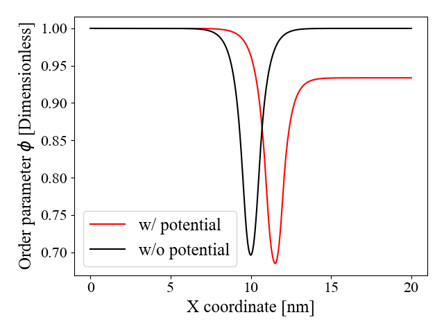
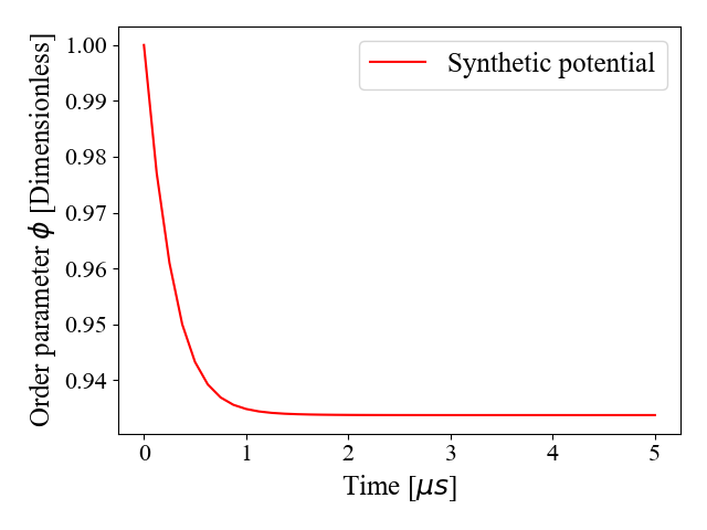
From Fig. 1a, we see that minimum of has clearly shifted to the right, indicating rightward GB migration, as expected. We also notice that the added potential manifests as an asymmetry in with in the right grain. As the GB migrates, the value of in the right grain decreases gradually and converges to its steady-state value, as evidenced in Fig. 1b. The lower value of in the right grain is a consequence of the synthetic potential, interpreted as energy due to SSDs, added to the right grain. While at the continuum scale SSDs do not result in lattice distortions, at the atomic scale, they contribute to disorder. Since describes disorder, the prediction that in the right grain is in line with the physical interpretation of . The synthetic potential constructed in this paper allows us to induce migration of GBs surrounding a particular grain, identified by its crystal orientation, and can be used as a surrogate for many forms of driving forces due to energy differences, either coming from differences in SSD densities, stored strain energy, or plastic anisotropy.
Next, we leverage this example to compare the results from the current formulation to that by Admal et al. (2018). The time history plots of the GB displacements and measured coupling factor are shown in Fig. 2.
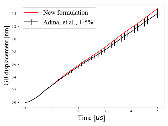
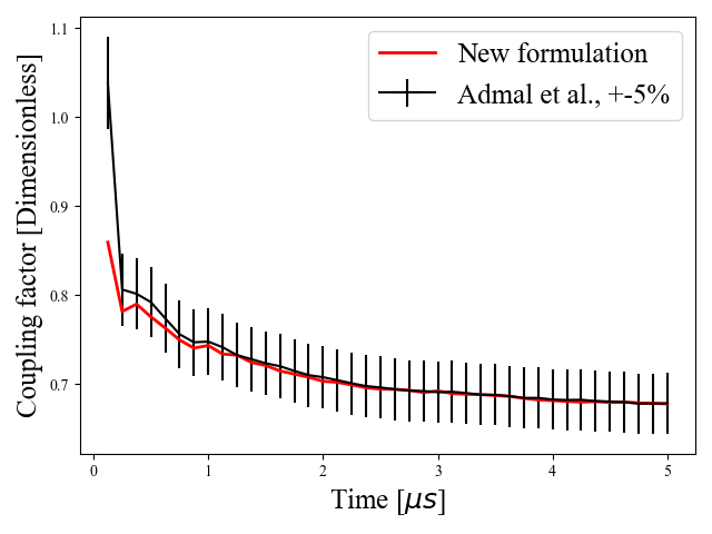
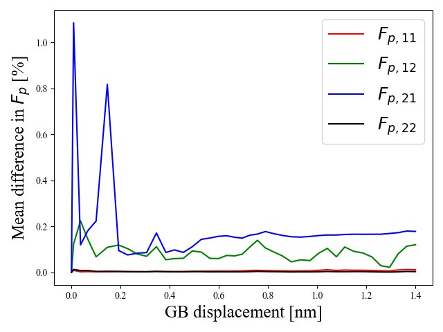
As evidenced by Fig. 2a, some differences in GB displacements are visible, but they remain below 5%. The fitted GB migration velocities reveal a 6.07% difference. However, the simulated coupling factor show good agreement, as shown in Fig. 2b. These observed differences are within acceptable ranges, and the difference in migration velocity can be compensated for in model parameter calibration. In Section 2.4, it was hypothesized that the solutions to Eq. (30) and Eq. (16) should yield identical evolutions for , we now check the validity of this hypothesis with simulation data. Recalling that GB plasticity (which is what measures) is due to GB migration, we plot the mean percent difference in components of as a function of the GB displacement, see Fig. 2c. The plot of the mean differences in components of shows good agreement between the evolution histories computed from the two formulations, thus confirming our hypothesis.
3.2 Performance comparison
In this example, we compare the computational cost of the current formulation to that by Admal et al. (2018) using a similar model problem as discussed in the previous section, where the scaling of total number of DOFs and simulation time are measured. We limit our comparison to the framework by Admal et al. (2018) since it is closely related to our current work and includes identical physics. It is true that many other models for GB migration exist, but a comparison of numerical efficiency is not fair unless the models being compared include similar physics. To this end, it is appropriate to compare our work with some dislocation-based models such as Zhang and Xiang (2018) and Zhang and Xiang (2020), and disconnection-based models such as Runnels and Agrawal (2020) and Gokuli and Runnels (2021). However, as those models are still under active development and are not formulated for numerical efficiency, further comparison is not pursued here.
In order to explore the scaling of our formulation, we change the size of the bicrystal to a square with an edge length of 20 nm and consider a sequence of uniform meshes with elements, generated using the sequence . All other simulation settings are identical to that described in Section 3.1. A plot comparing the number of DOFs in each mesh, and the corresponding simulation time is shown in Fig. 3.
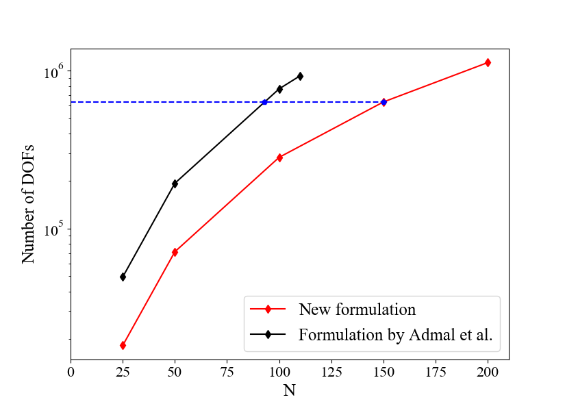
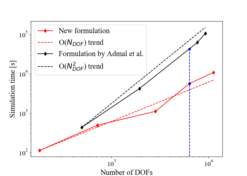
The reduction in the number of DOFs, and its dependence on is shown in Fig. 3a. In this example, the framework in Admal et al. (2018) requires a total of 19 DOFs (1 for , 2 for , 12 for and 4 for ) per node. While using the current formulation, the number of DOFs per node is reduced to 7 (no DOFs related to ), which is a 63.2% decrease. The reduced number of DOFs in turns leads to a huge decrease in simulation time, as evidenced in Fig. 3b. Apart from the direct advantage that the new formulation yields fewer number of DOFs for a given mesh, it is interesting to note that even when the number of DOFs are identical (e.g., two blue points in Fig. 3a), the new formulation has a shorter run time (e.g., comparing the two blue points in Fig. 3b, shows that the simulation time of the formulation by Admal et al. (2018) is about 6.6 times longer). We hypothesize that this additional gain in performance is due to the change in sparsity pattern (hence the bandwidth) of the system matrix associated with fewer DOFs per node, as the solution time for sparse matrix solvers depend both on the system size and its sparsity pattern. It should be noted that although the scaling test was performed on a simplified geometry, similar performance enhancements are expected in general. The reason for this claim is that the performance gain roots from the reduced number of DOFs per node, which is independent of the underlying geometry or the polycrystal system. This significant increase in computational efficiency, resulting from fewer DOFs per node and improved sparsity pattern, is beneficial in many ways. For more complex crystal configurations, a refined mesh near the GBs is desired to resolve high local gradients. The current formulation relaxes the requirements on computational cost, giving room for the use of a more locally refined mesh. In addition, reduced number of DOFs entails less memory usage during the simulations.
3.3 Evolution of a circular tricrystal
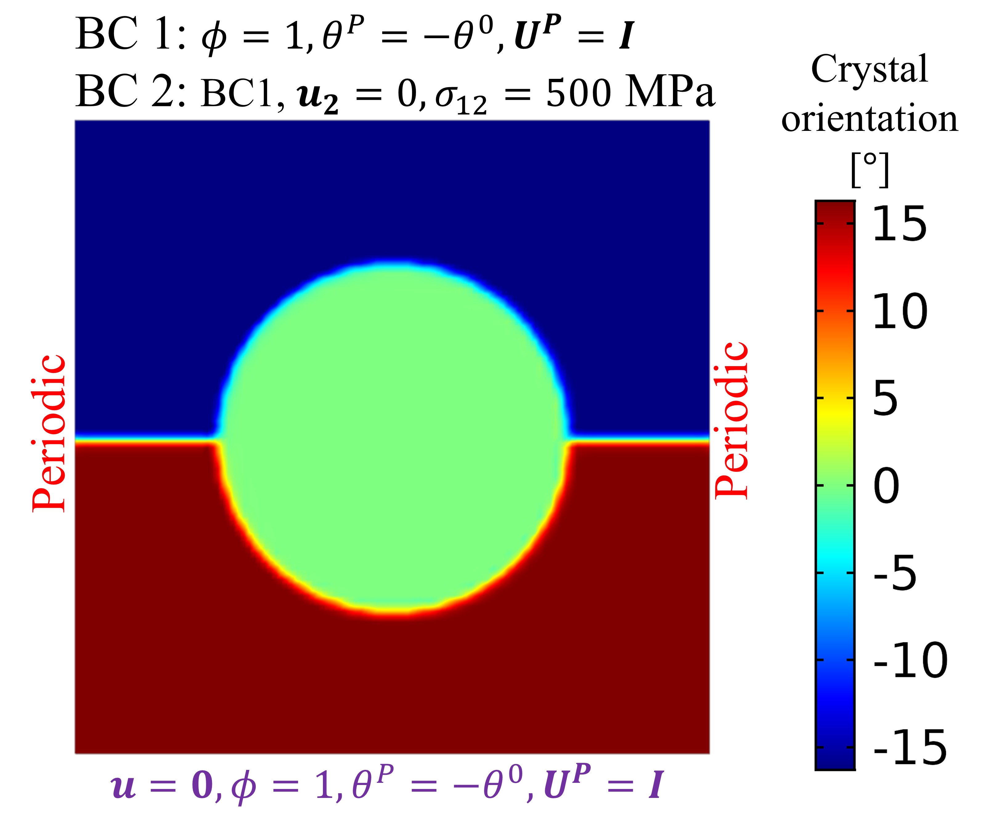
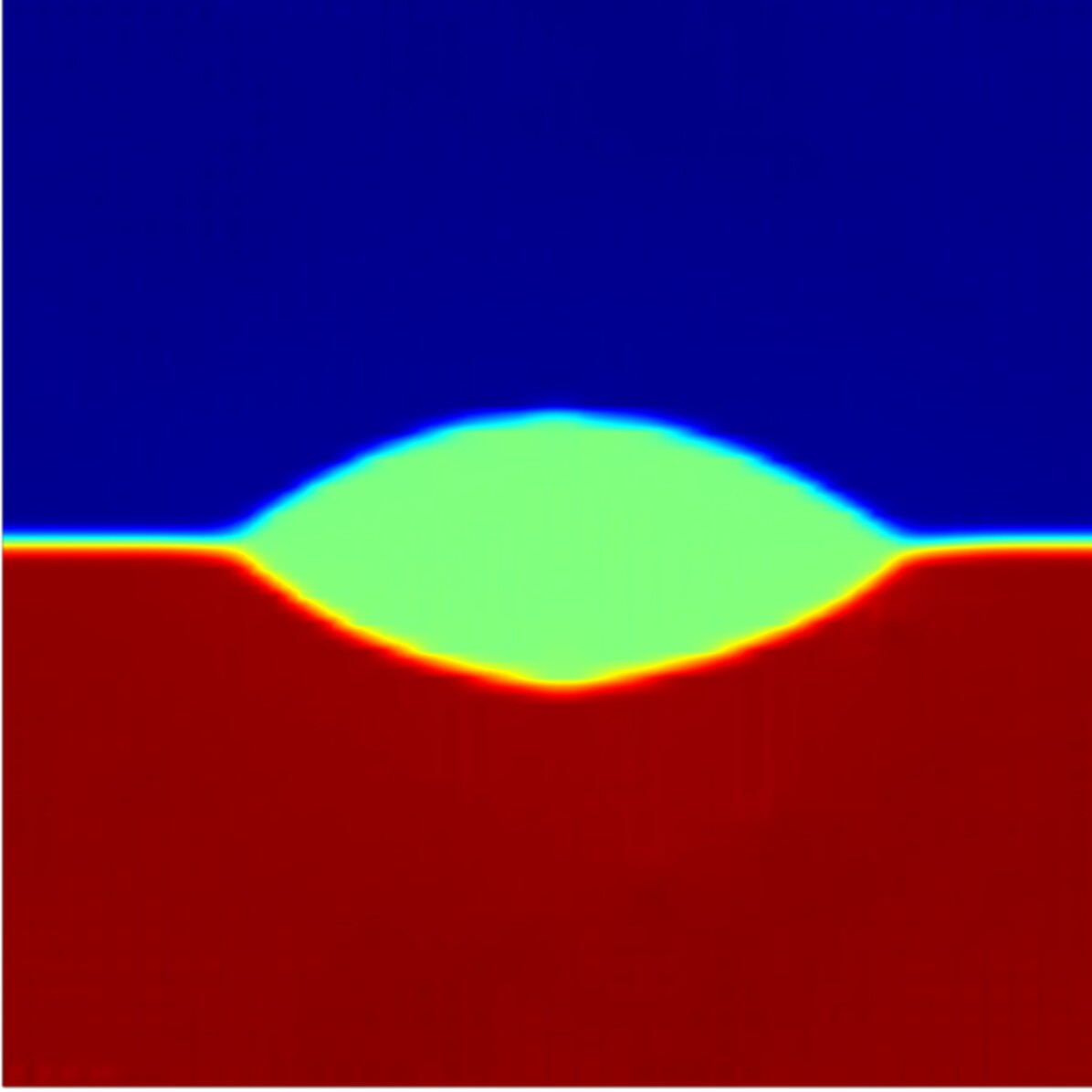
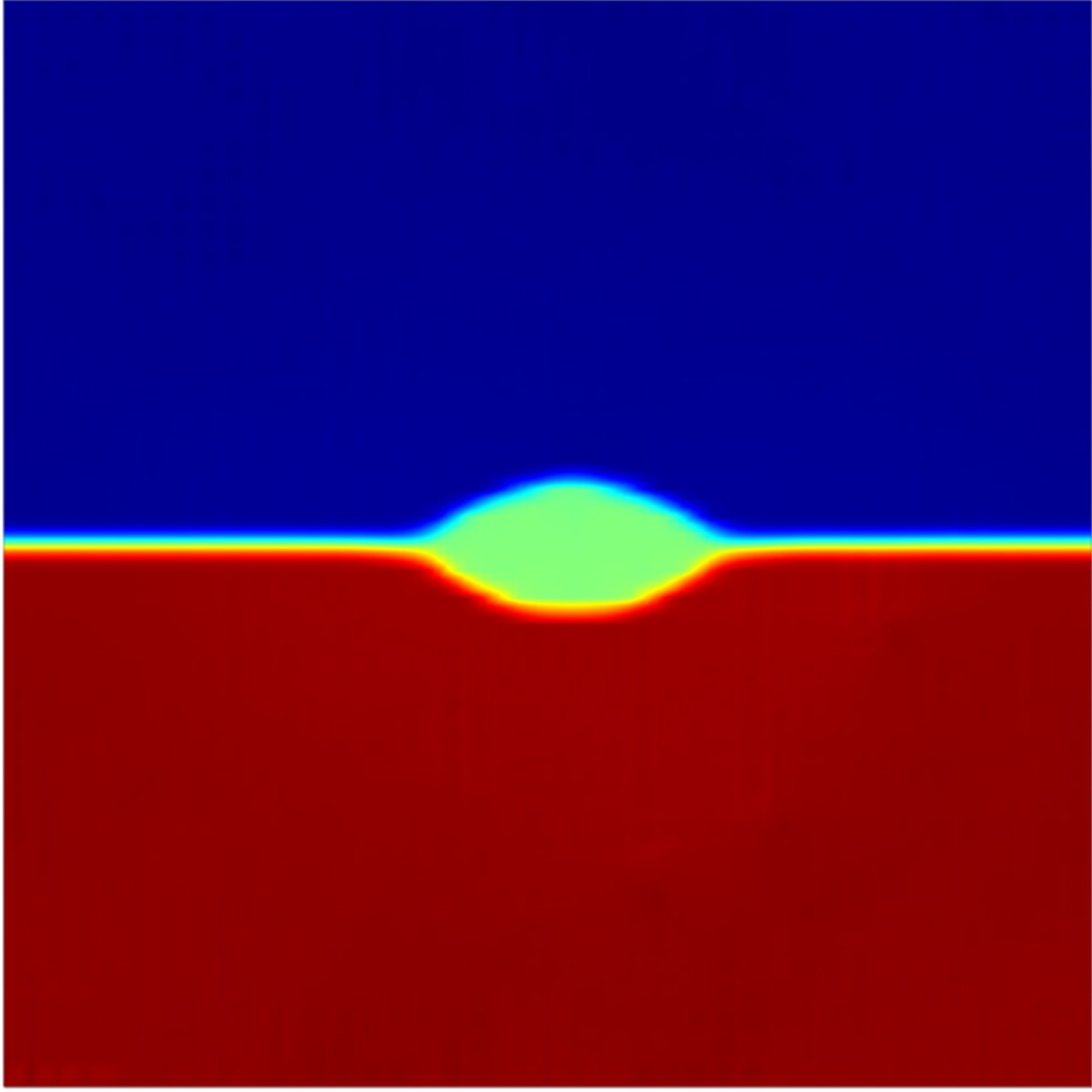
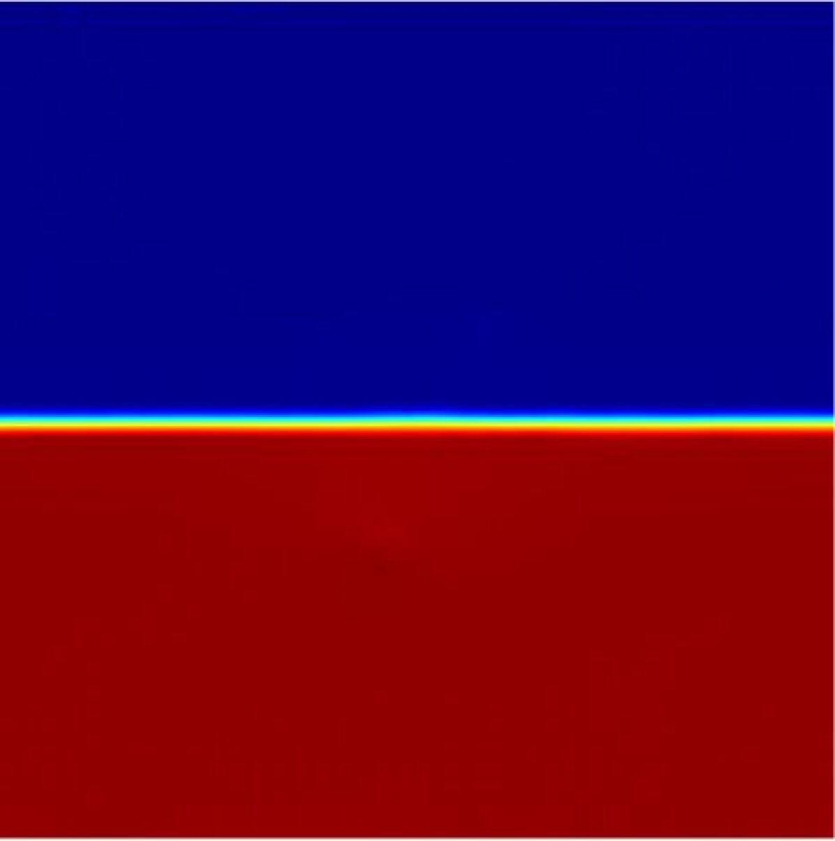
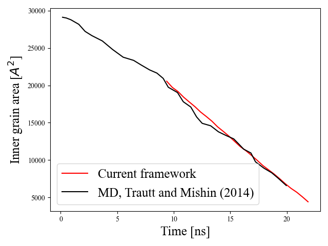
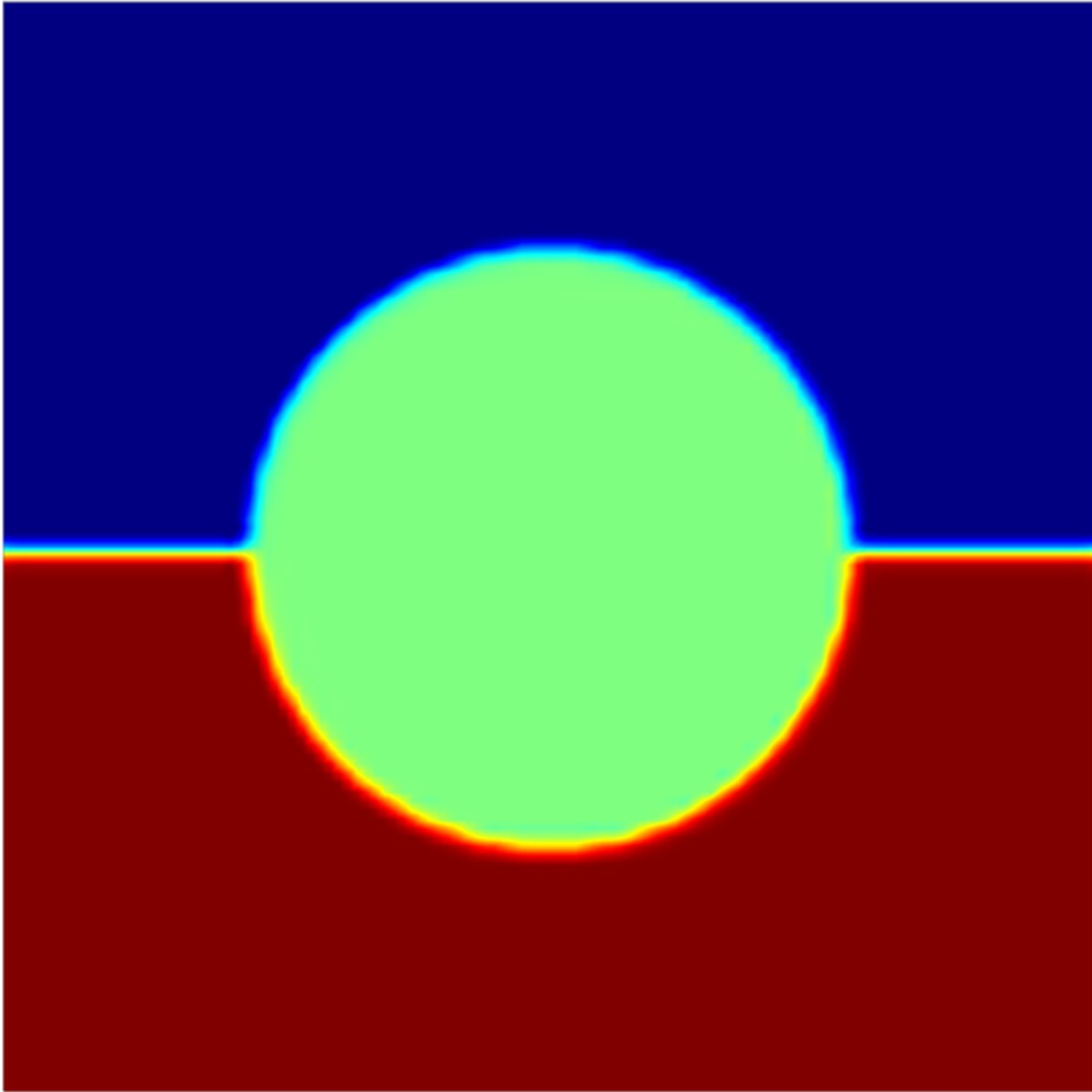
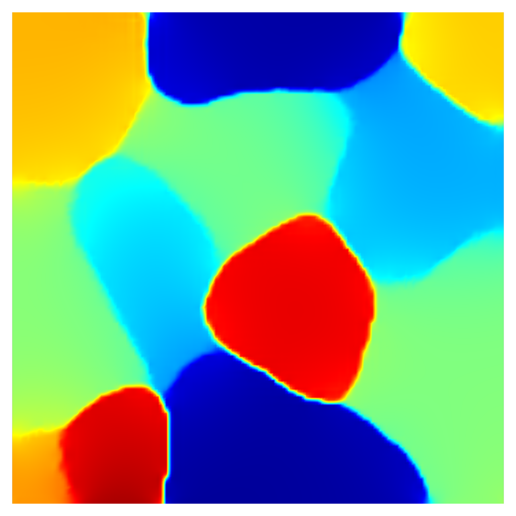
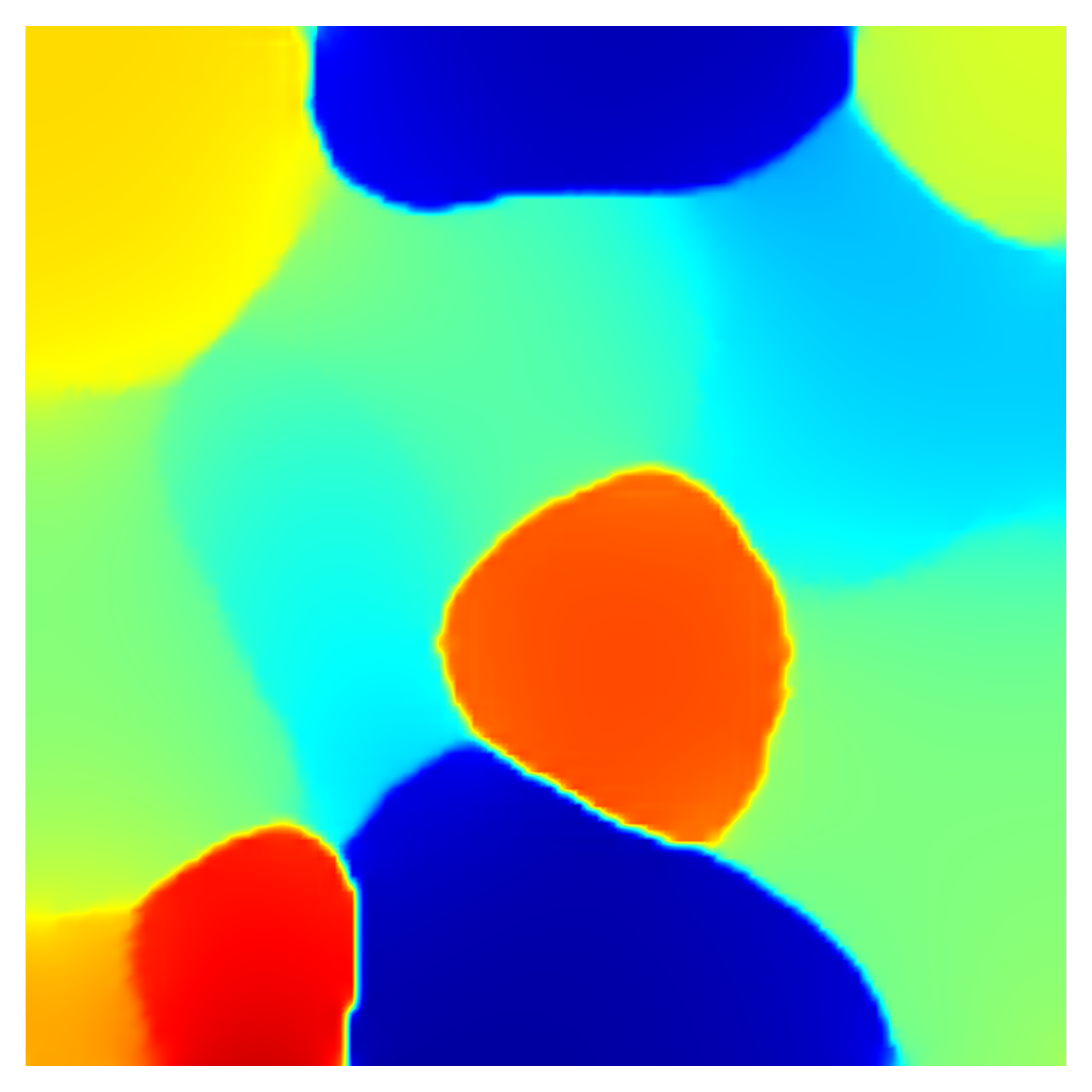
In this example, we study the evolution of a copper tricrystal, originally constructed by Trautt and Mishin (2014), that is formed by embedding a circular grain into a bicrystal, as shown in Fig. 4. In particular, we make a quantitative comparison with predictions from MD, and explore the effect of shear stress on the GB motion and grain rotation. All results are are compared to the MD simulations by Trautt and Mishin (2014).
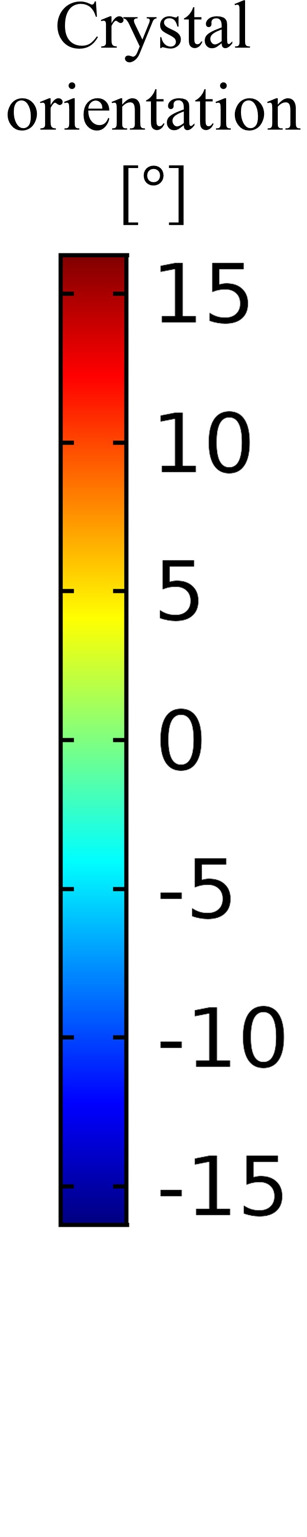
The three grains are oriented such that their crystal directions are all aligned along the -axis pointing vertically out of the page. A circular grain of radius 8.33 nm with an orientation of 0∘ is placed in the center of a square bicrystal of side length 30 nm, whose upper and lower grains have orientations of 73.74∘ and 16.26∘, respectively. The crystal direction for the center grain is parallel to the -axis. The computational domain is discretized with quadratic Lagrange elements. This configuration corresponds to Case 1 in the MD study by Trautt and Mishin (2014). We note that due to the four-fold symmetry of the cubic crystal, the orientations of the grains are not uniquely defined, and this manifests as non-uniqueness of the GND density. For example, the orientations described above result in a larger GND density for the upper semi-circular grain boundary relative to its lower counterpart, while changing the orientation of the top grain to an equivalent results in equal misorientations and GND densities. Since the two semi-circular GBs have identical atomistic structures, and therefore equal energies, we proceed with the latter choice. The tricrystal is equipped with three slip systems with equal inverse mobilities, and oriented along directions given by Eq. (32) with , , and . To match the initial grain shrinkage rate as observed in MD by Trautt and Mishin (2014) (cf. Figure 8b therein), the inverse mobility for , , and the maximum slip mobility, , were calibrated as and , respectively. All other simulation parameters are identical to those listed in Table 1, except that no synthetic potential is applied.
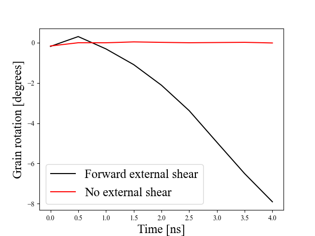
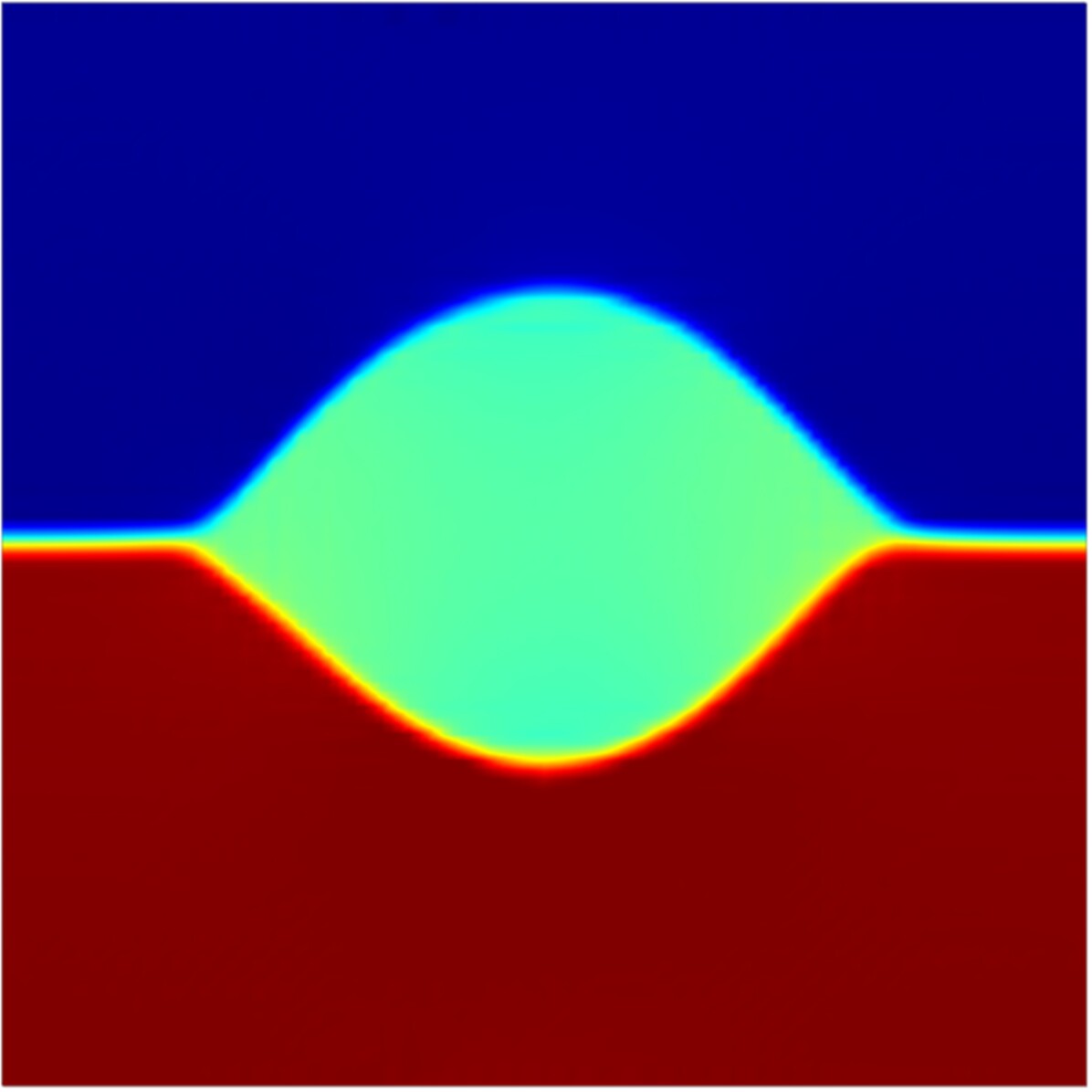
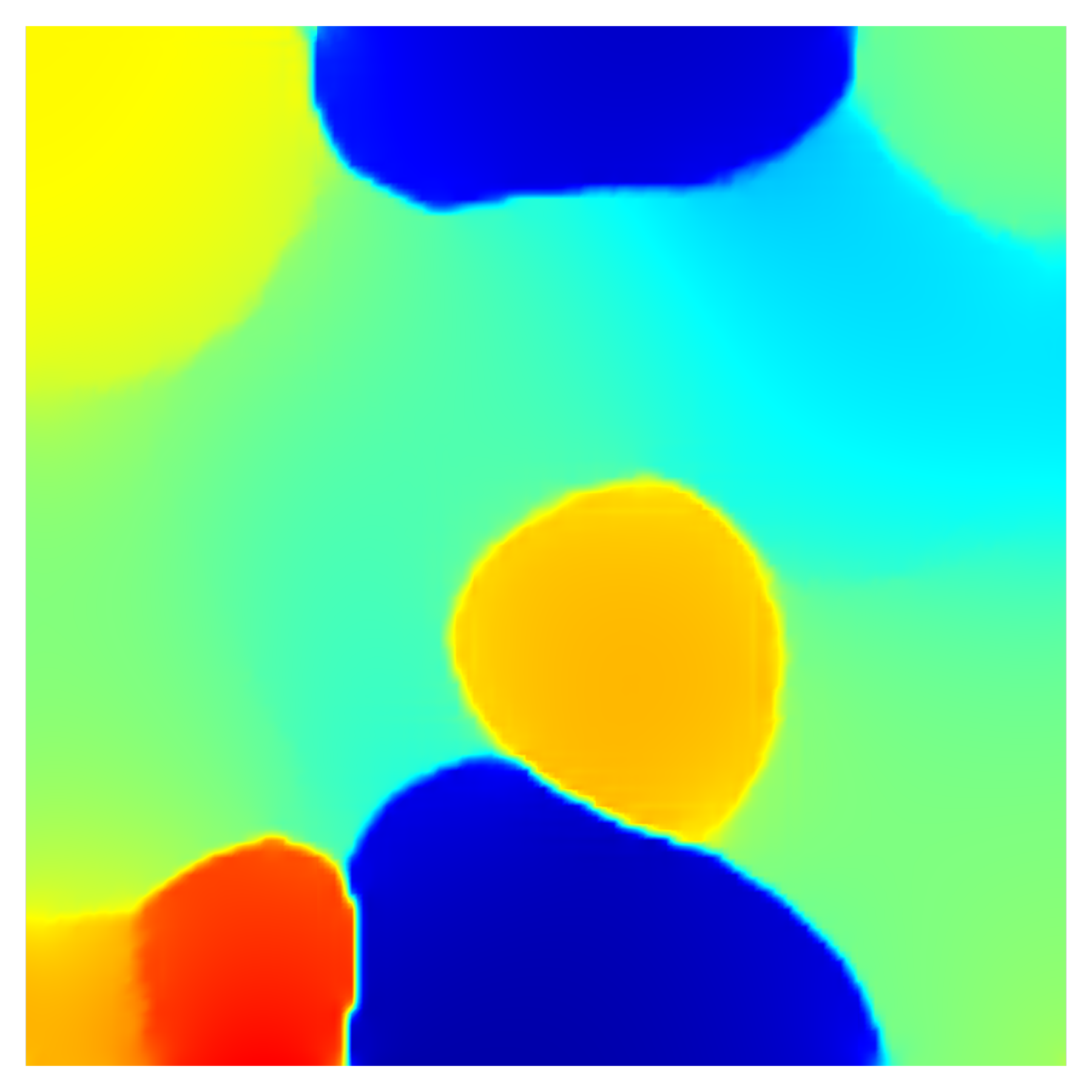
A schematic showing the initial crystal orientation and the applied boundary conditions is shown in Fig. 4. Two cases are considered, one with no external loading, and the other with an external shear of 500 MPa acting on the top surface, and the system is evolved for 19 ns and 14 ns, respectively. Selected snapshots of crystal orientations during their evolution for the two load cases are shown in Fig. 5 and Fig. 7, where the latter corresponds to the case of applied shear. Fig. 6 compares the variations of grain area and rotations as functions of time for the two load cases.

|
|
|
|
|
|
|
|
|
|
From Fig. 5, we note that in the absence of external loads the two semi-circular GBs, driven by curvature, evolve at identical speeds preserving the symmetry of the grain microstructure. Moreover, the orientation of the grains are preserved throughout the simulation as shown in Fig. 6b. As noted in Section 2.3, the GB motion observed in this simulation may be interpreted as a superposition of coupled GB motion and GB sliding that produces no grain rotation. These features, which are also observed in MD simulations of Trautt and Mishin (2014), can be attributed to coupling factors that are equal in magnitude but opposite in sign for the two GBs, resulting in no grain rotation. In the absence of grain rotation, the equivalence (energetic and kinetic) of the two GBs is preserved, and they continue to evolve with equal speeds. In addition, the evolution history predicted by the continuum simulation is in close agreement with that observed by MD simulation, which proves that the framework can produce accurate results after material parameter calibration.
In the case of shear-driven tricrystal, the GBs experience a driving force due to shear stress in addition to the force due to curvature. Fig. 7 shows that the planar GB migrates upward due to the external driving force. For the lower semi-circular GB, both the curvature and shear stress drive the GB upwards, whereas for the upper semi-circular GB, the two driving forces have a tendency to drive the GB in different directions (curvature flow drives the GB downwards, while shear stress drives it upwards). This leads to a difference in migration velocities, with the lower GB migrating faster than the upper one. This difference in migration velocities, along with GB coupling, leads to a nonzero net rotation rate for the center grain, in the direction such that its crystal orientation is decreased. When comparing the continuum simulation results with those by MD, we see that the two agree qualitatively, i.e., the planar GB migrates upward, the lower GB migrates at a faster rate than the upper one, and the inner grain decreases in orientation.
The qualitative agreements between continuum and MD simulations discussed above provide confidence for the model to be used in more complex scenarios. While using GB energies and mobilities obtained from atomistics would yield a quantitative comparison with MD simulations, we do not pursue such a study due to certain limitations of our framework, which we will now discuss. In our framework, since the construction of GB energy is in terms of the GND density, and the norm of the GND density increases monotonically with GB misorientation, our model is only applicable for small angle GBs. In the tricrystal example, although the misorientations computed using the originally prescribed orientations (, and ) are large angles, the cubic symmetry enabled us to identify them with small angles by noting the equivalence of grain orientations and , resulting in the correct GND density that accurately reflects the GB energy. While such an unambiguous choice of GND density is possible for small angle GBs, it is not possible for large angle GBs. For example, consider a tricrystal with grain orientations , and . Using cubic symmetry, we note that all GBs are equivalent with misorientation angle of . On the other hand, no choice of orientations among their equivalent classes will result in equal misorientations for the three GBs. Therefore, our framework limits us to small angle GBs with a Read–Shockley type GB energy. In Section 4, we discuss how our dislocation-based GB model can complement a disconnection-based framework to model GBs with arbitrary misorientations.
Finally, we remark that the mobility of a GB depends on through the relation given in Eq. (26), which results in the qualitatively correct trend, where GBs with larger misorientation have higher mobilities Trautt and Mishin (2014).101010MD simulations from Trautt and Mishin (2014) highlight the importance of misorientation-dependent GB mobilities in the shape evolution of the inner grain, especially when the two semi-circular GBs have vastly different misorientations. However, we note that the mobility of the GB also depends on orientations of the slip systems relative to the GB. Therefore, in order to make detailed quantitative comparison between our model and MD, further material model parameters (e.g., , , and the functional form of as a function of ) calibration is necessary.
3.4 Evolution of a polycrystal
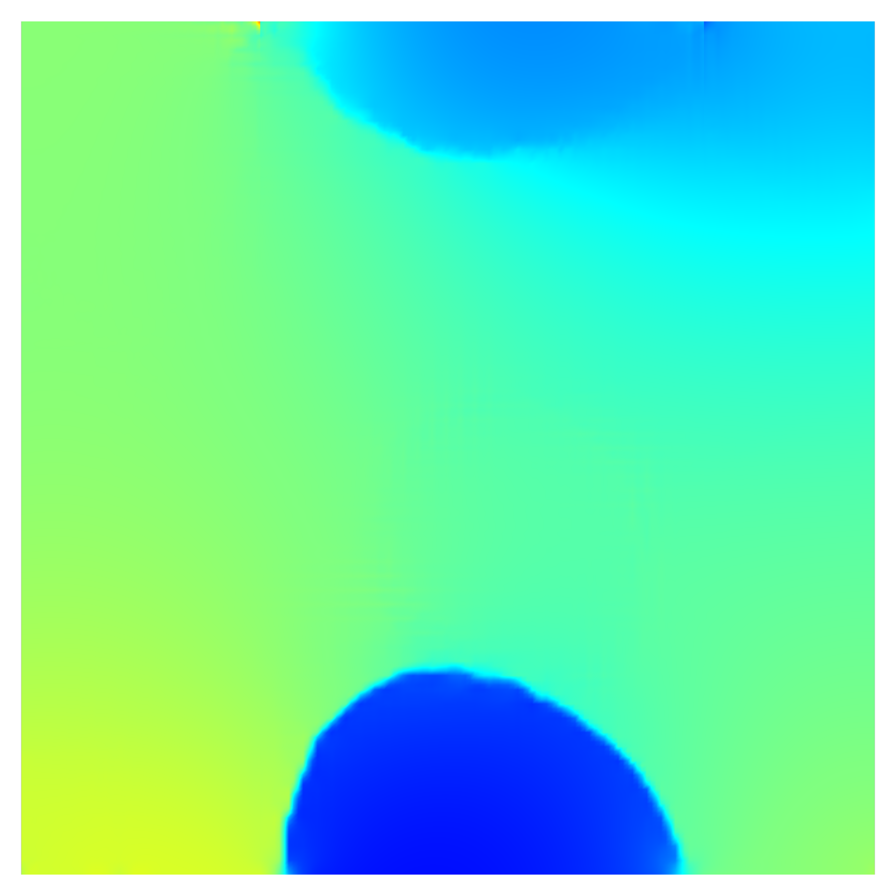
In this last simulation, we study the evolution of a square polycrystal under two different loading cases. In the first case, no external load is applied. In the second case, a displacement boundary condition is imposed to intentionally induce grain rotation. The evolution of texture in the two cases are compared, and the importance of external loads in GB evolution is highlighted.
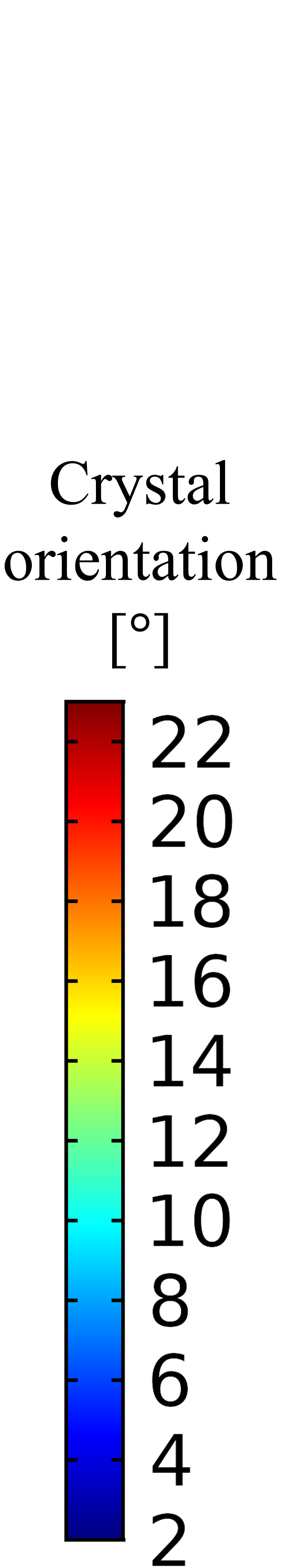
The computational domain is a square polycrystal of side length 100 nm with 13 grains, generated using DREAM.3D (Groeber and Jackson, 2014).111111DREAM.3D is an architecture for computational microstructure tools that allows users to create ’recipes’ or pipelines for processing digital instances of microstructure. The domain is discretized by quadratic Lagrange elements with a uniform mesh size of 1.6 nm. The crystal orientations are drawn at random from a normal distribution with a mean of 22.5∘ and a standard deviation of 10.5∘. Additional checks are performed to limit the GB misorientations to the range 5∘ to 20∘, which ensures that all GBs are within the small angle misorientation range to which our model is applicable. The global X- and Y-axes are assumed to coincide with the and directions of a single face-centered cubic (fcc) crystal, such that the in-plane effective slip directions are given by Eq. (32) using , , and (Kysar et al., 2010). Other simulation parameters are identical to those listed in Table 1, except that no synthetic potential is applied.
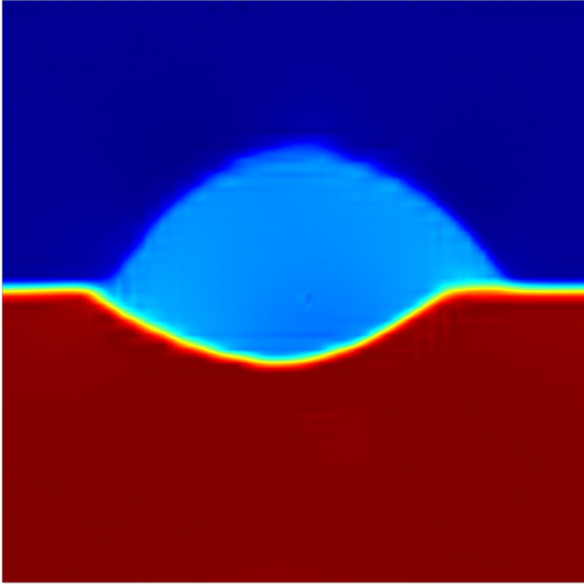
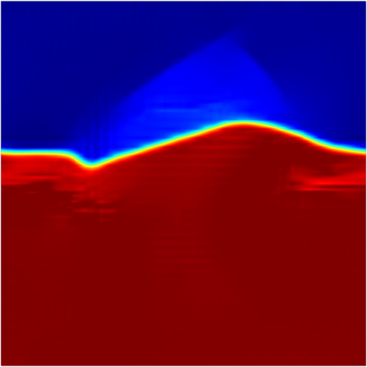
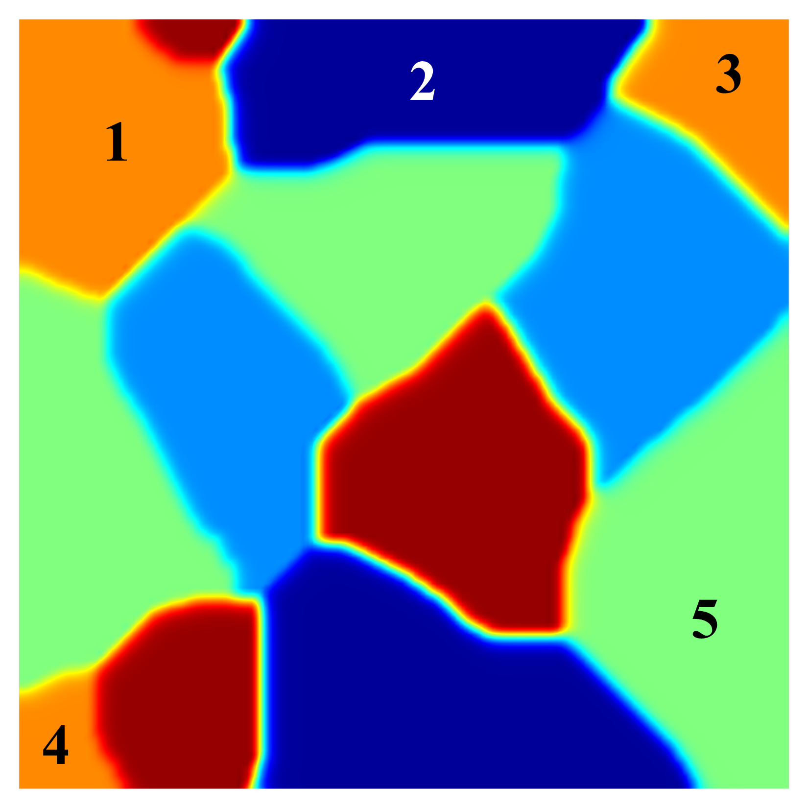
A schematic of the polycrystal with a color density plot of initial grain orientations along with applied boundary conditions for the two loading cases is shown in Fig. 8a. The GND density corresponding to the initial grain orientation is shown in Fig. 8b. Since all GBs in the system are low-angle GBs, the norm of the GND tensor serves as a valid measure of GB misorientation. The two loading cases are simulated using boundary conditions imposed on the top edge of the polycrystal. In the first case, the top edge is traction-free, while in the second case, a vertical displacement of 4 nm is imposed on a part of the boundary, shown in red in Fig. 8a, at a rate of nm/s. In both cases, the bottom edge of the domain is held fixed. The duration of the simulation is set to be s in both cases.
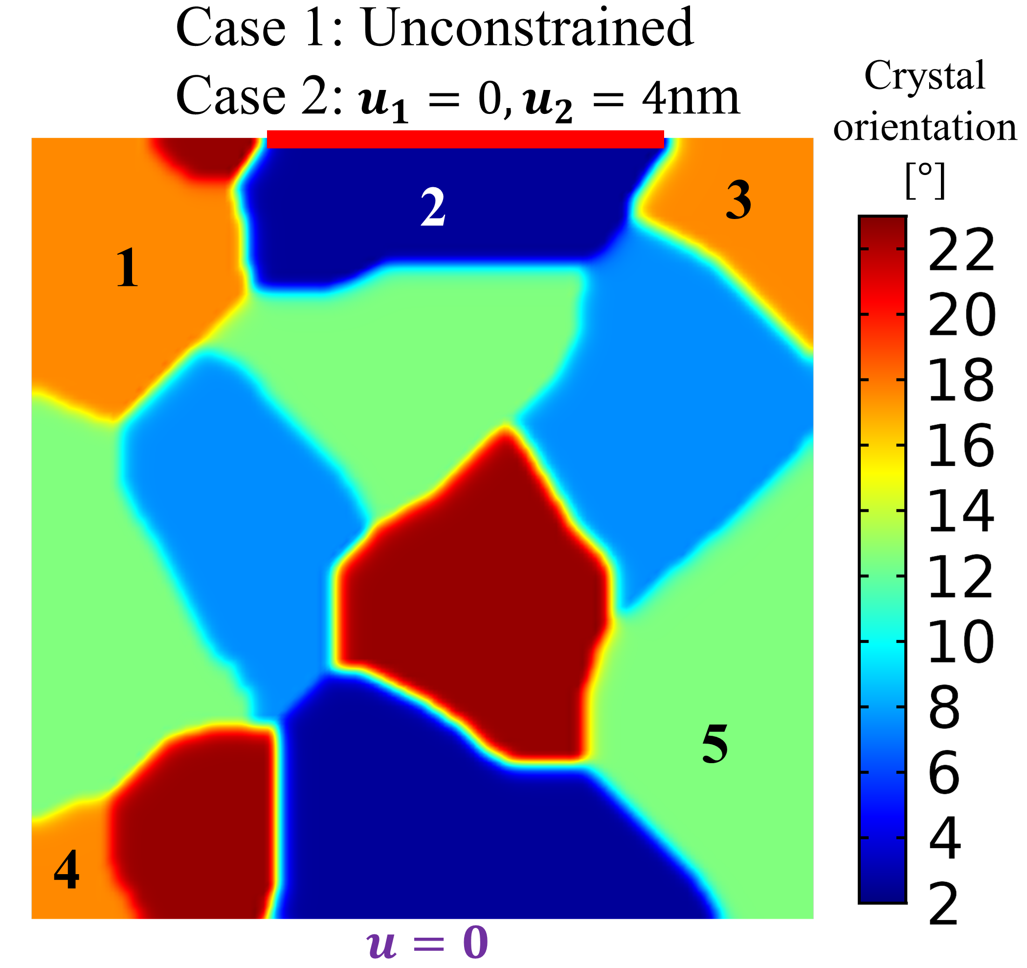
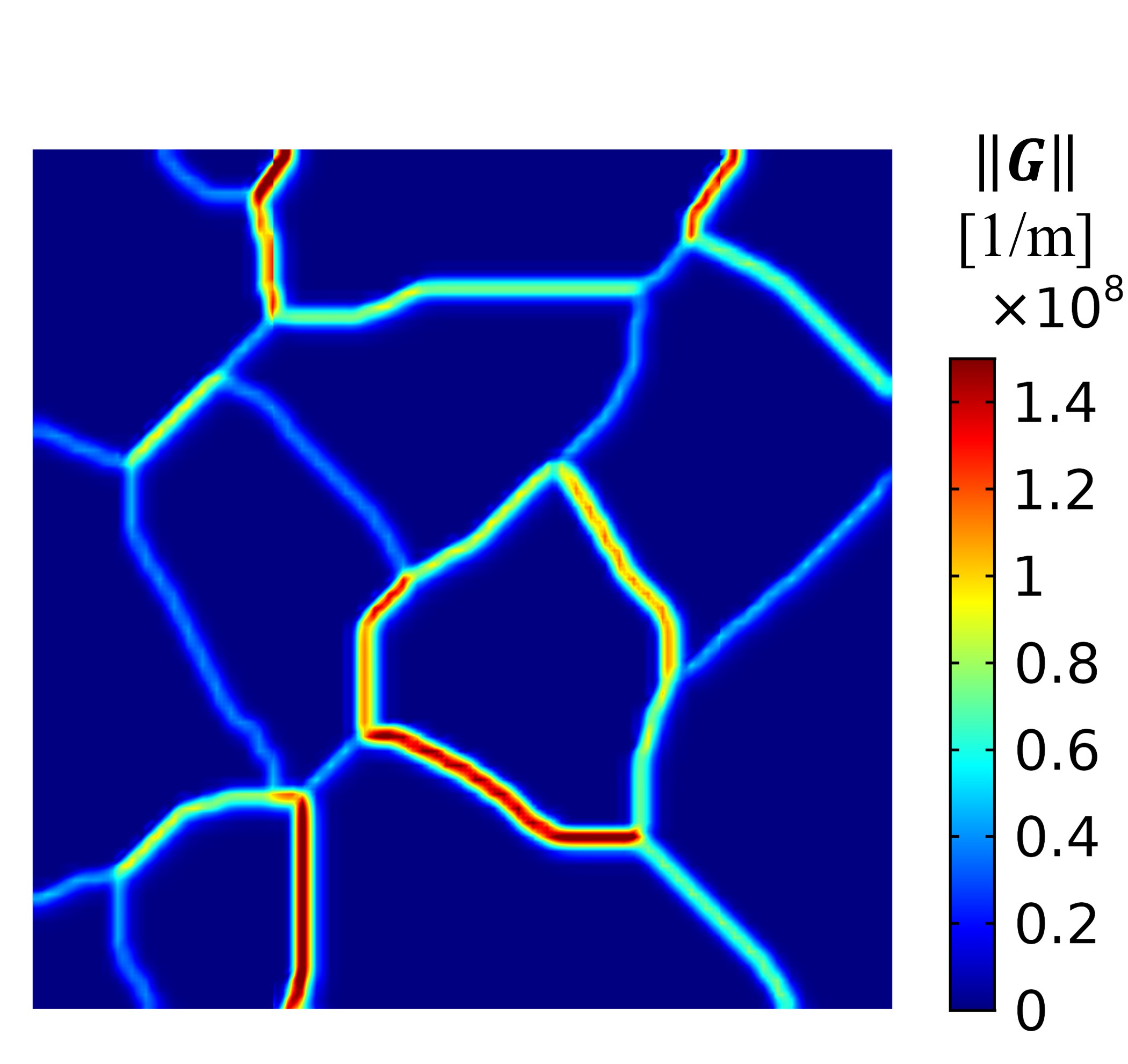
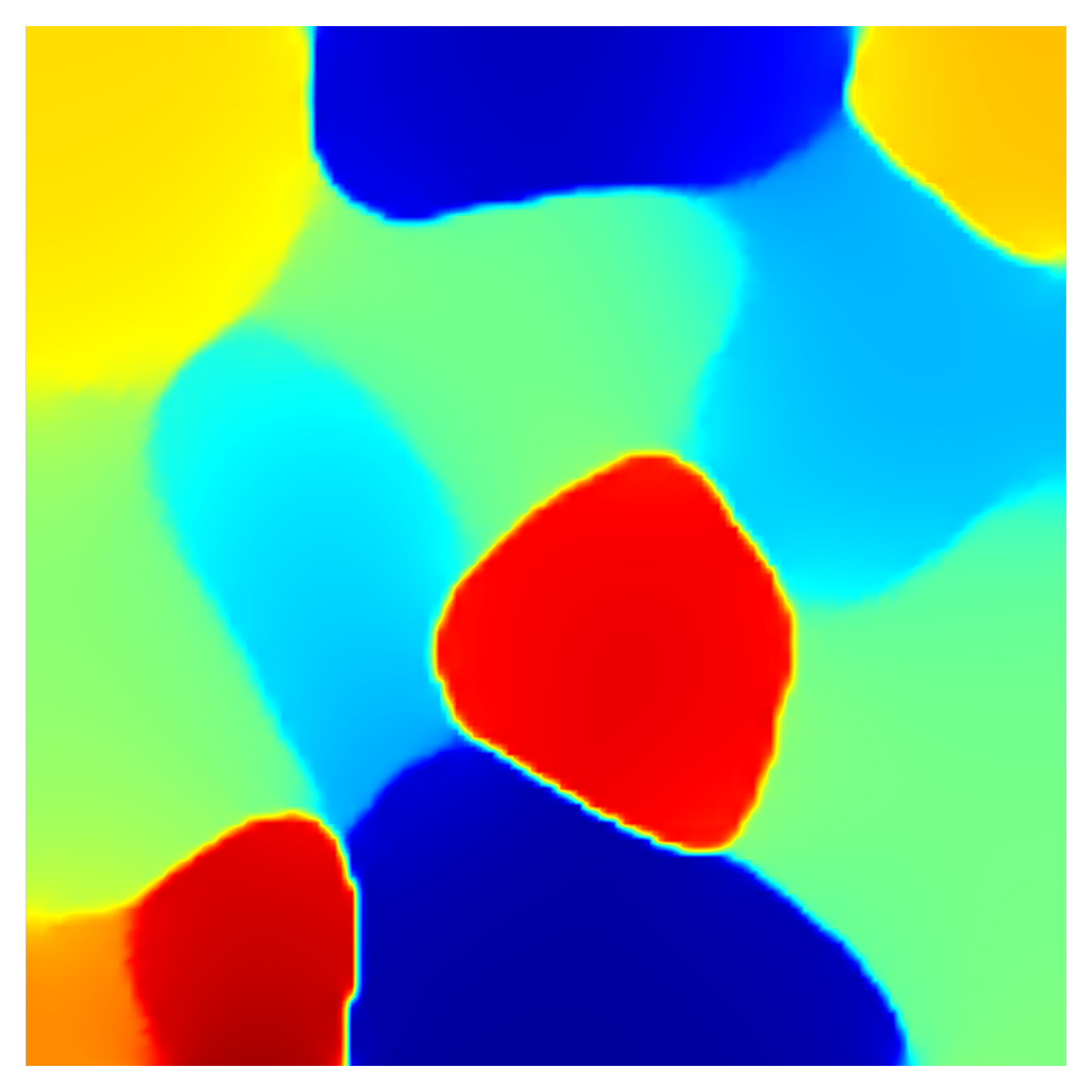
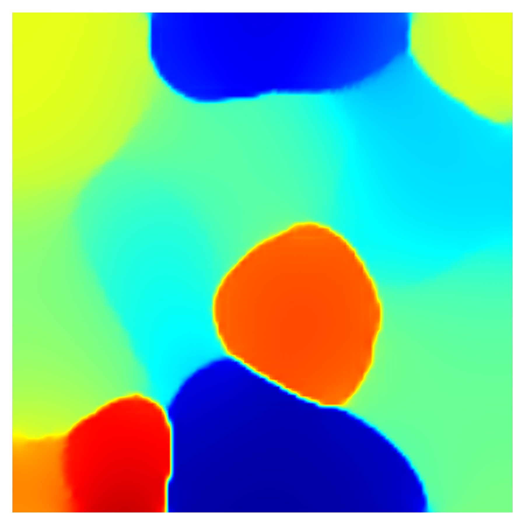
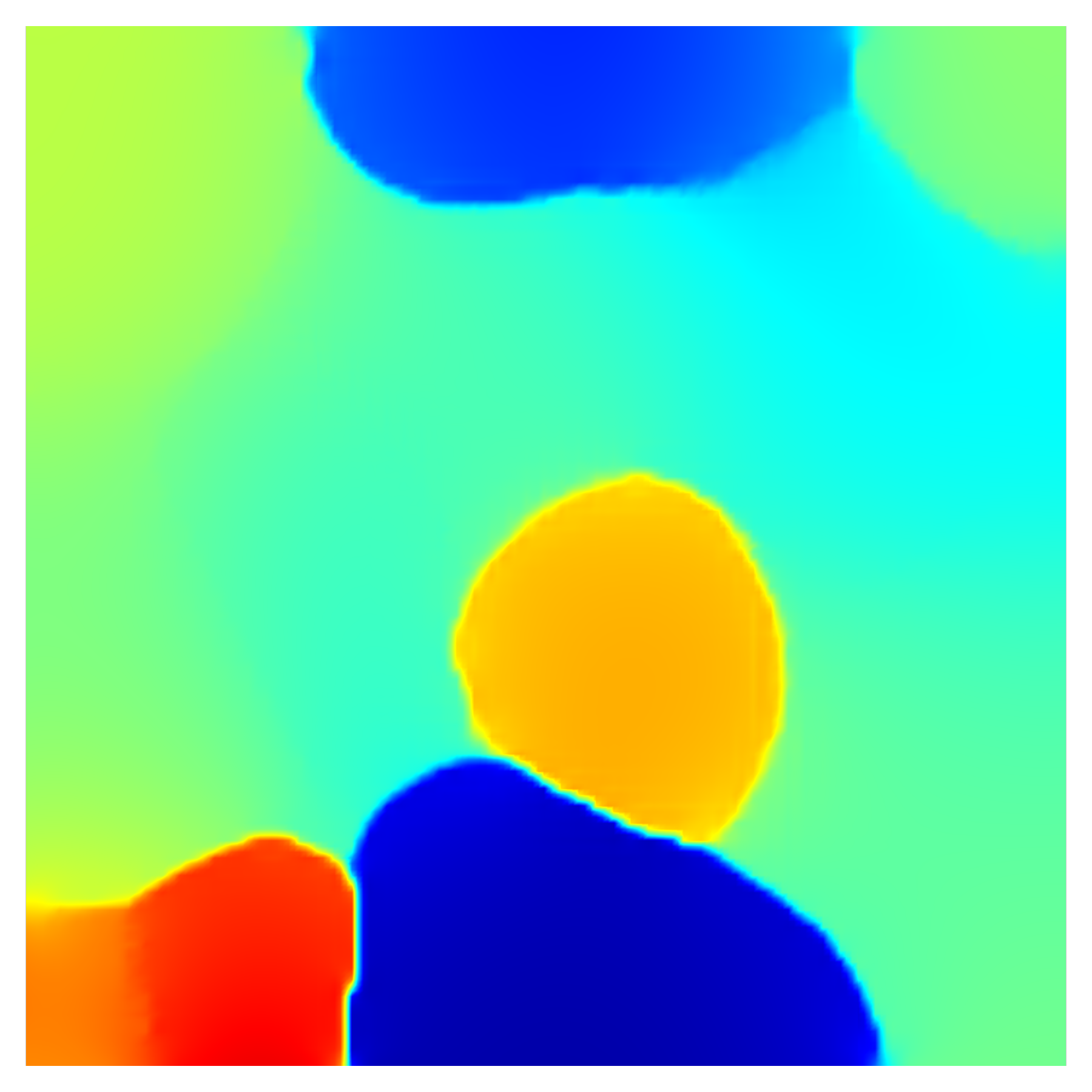
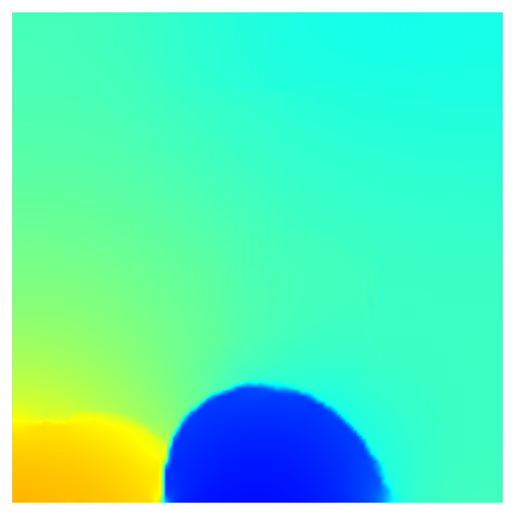
Fig. 9 and Fig. 11 show snapshots (taken at the same time instances) of the time evolution of grains under no external load and uniaxial load cases, respectively. Clearly, in both cases, GB evolution is accompanied by grain rotation. However, we note that uniaxial loading has a noticeable impact on the rate of grain rotation. For instance, a comparison of Fig. 9d and Fig. 11d shows that while grain 1 rotates to decrease its misorientation with the neighbouring grains, the rate of lattice rotation is lower in the presence of external loads. This can be seen in Fig. 9d wherein grain 1 ceases to exist by merging with its neighbor by s, while it is still visible in Fig. 11d. The above observation extends to grain 4 as well.
|
|||
 (a)
(a)
|
 (b) s
(b) s
|
 (c) s
(c) s
|
|
 (d) s
(d) s
|
 (e) s
(e) s
|
 (f) s
(f) s
|
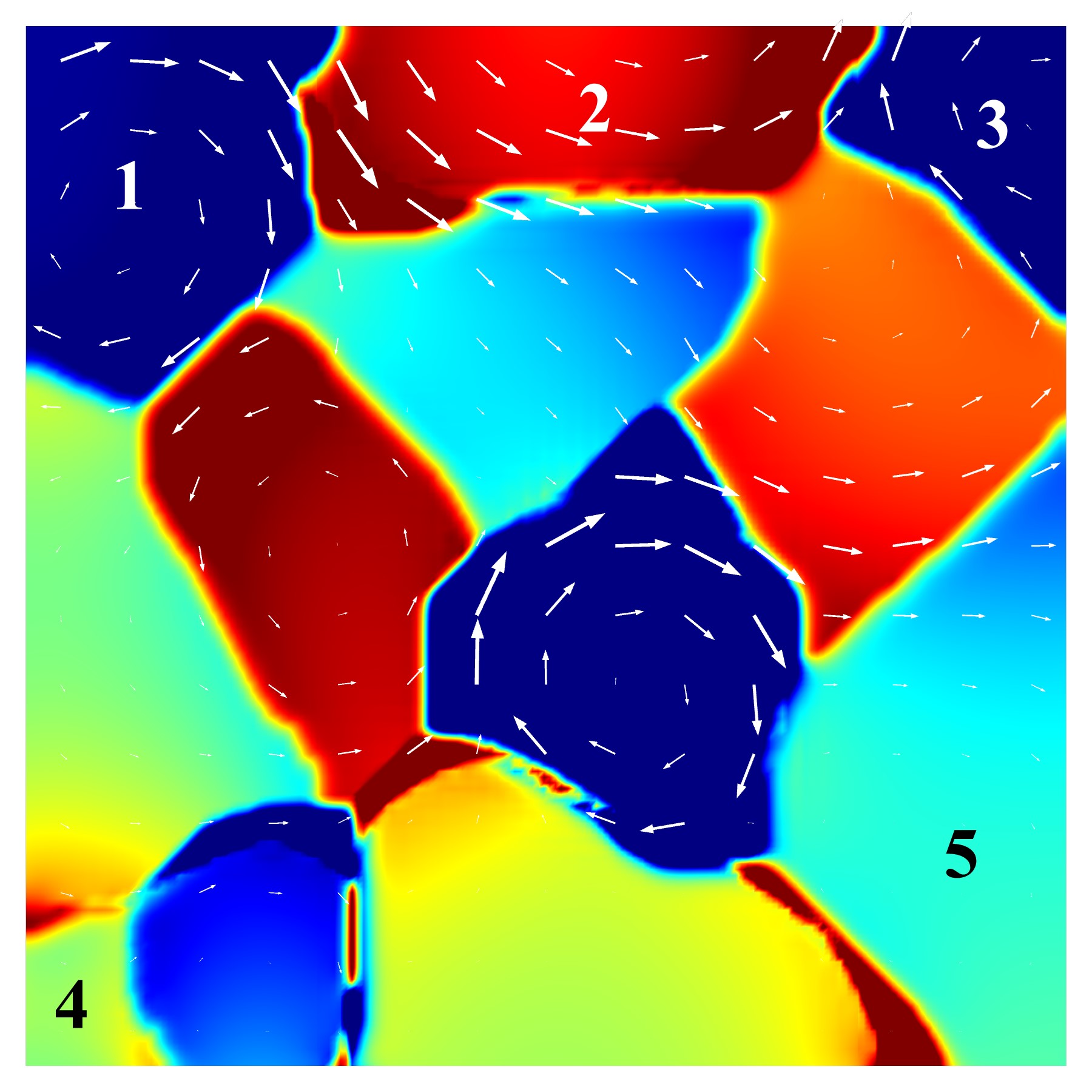
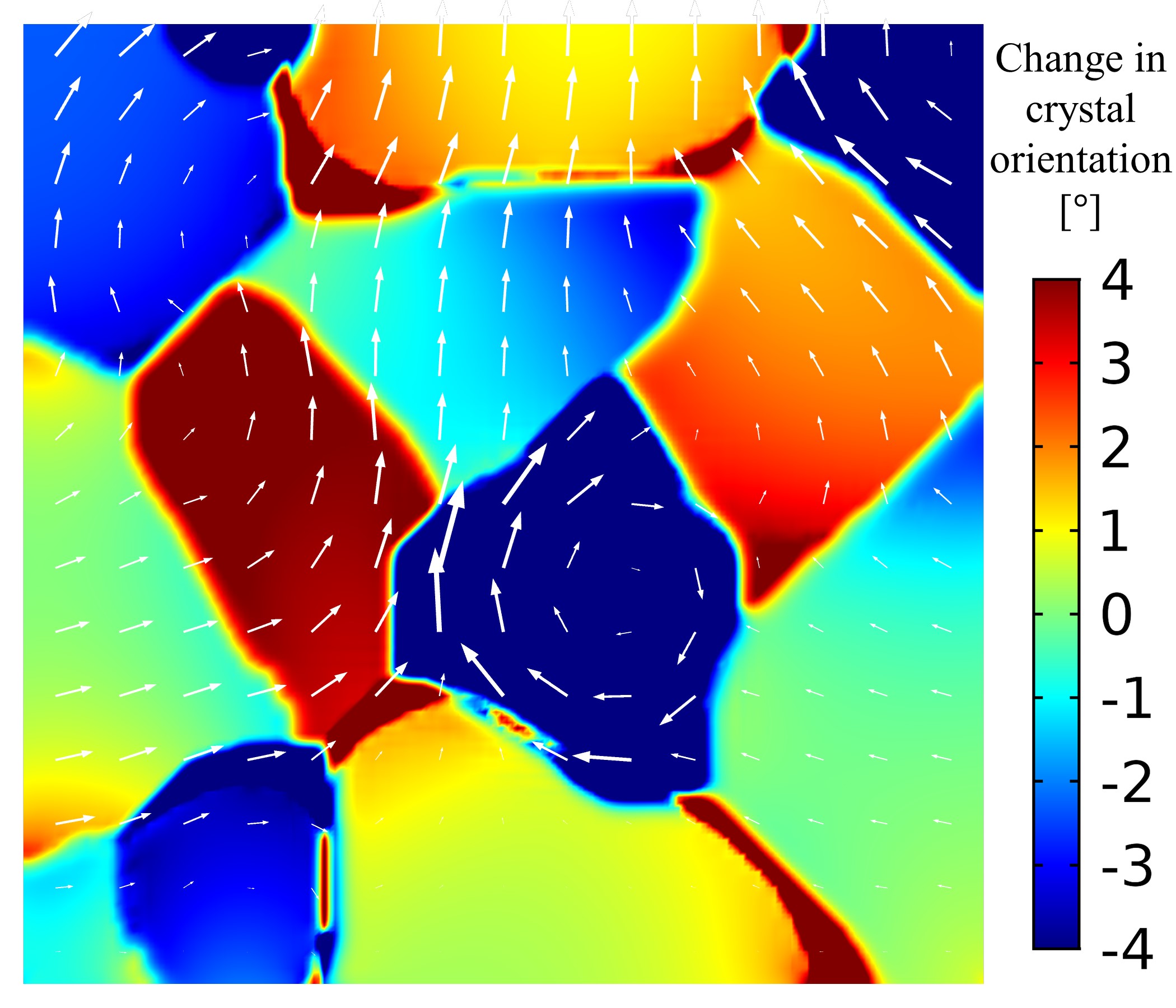
The effect of external load on grain rotation is more evident in Fig. 10, which compares grain lattice rotations for the two load cases at time s. The arrows in Fig. 10 depict displacement vectors. From Fig. 10a, we note that in the absence of external load, lattices of grains 1 and 3 rotate clockwise, while the lattice of grain 2 rotates counterclockwise. On the other hand, Fig. 10b shows that the presence of an external load on grain 2, superimposes a counterclockwise rotation in grain 1 and a clockwise rotation in grain 3. This results in a reduced lattice rotation for grain 1 while the lattice rotation is enhanced in grain 3. Moreover, lattice rotation of grain 2 is partially suppressed in the presence of external loads.
|
|
|||
|
(a)
|
 (b) s
(b) s
|
 (c) s
(c) s
|
|
 (d) s
(d) s
|
 (e) s
(e) s
|
 (f) s
(f) s
|
In addition, additional rotations are introduced to grains 4 and 5, causing them to slightly rotate in the negative and positive direction, respectively.
In this simulation, equal mobilities are assigned to all available slip systems for simplicity. The work by Thomas et al. (2017) highlights the importance of GB-specific migration behaviors in polycrystal evolution by the MD simulation of a simple toy polycrystal. As shown in Admal et al. (2018), the migration behavior of a GB (e.g., geometric coupling, sliding, or a mix of both) within this framework can be controlled numerically by the available slip systems. For example, it was shown that having two slip systems instead of three, would result in motion by curvature with no grain rotation. Within our framework, various GB mobilities can be explored by having a spatially varying field (see Eq. (26)), as guided by experimental measurements or individual MD simulations Thomas et al. (2017), thereby allowing different migration behaviors for GBs in the system.
It is worth noting that the polycrystal simulation reveals a drawback of the diffuse-interface KWC-based models. During the evolution, as the misorientation of the GB decreases, the crystal orientation becomes more diffused. This can be seen in later stages of the two simulations (e.g., Fig. 9d and Fig. 11d). At these time instances, the crystal orientation field become diffused, which renders the identification of the location of GBs difficult. Note that similar diffused GBs can be seen in the polycrystal simulations by Admal et al. (2019). This can be mitigated by increasing the value of in Table 1, which is used to approximate the singular-diffusive term in Eq. (15). However, doing so stiffens the resulting PDEs and worsens the conditioning of the global system, hence it is not pursued here.
4 Conclusion and discussion
A computationally efficient framework for the simultaneous inclusion of grain boundary and bulk plasticity is proposed to simulate coupled polycrystal plasticity and grain boundary evolution. In this framework, which is based on the work of Admal et al. (2018), grain boundaries are represented by specialized arrangements of geometrically necessary dislocations that result in zero lattice strain, through the use of nonzero initial conditions for the lattice and plastic deformation gradients. This treatment encodes the grain orientation information into the plastic deformation gradient, and allows for the co-evolution of bulk and grain boundary plasticity using the evolution equation for the plastic deformation gradient in classical crystal plasticity theories. We introduced a synthetic driving potential within the framework, which allows us to drive the migration of a flat grain boundary without applying any mechanical loads, much like in molecular dynamics simulations. The primary difference between our framework and that of Admal et al. (2018) is that we no longer solve for individual slip rates, which in unison, give rise to grain boundary plasticity. Instead, their combined effect is formulated as a second-order differential equation for plastic distortion. As a result, slip rates on each slip system are no longer nodal degrees of freedom that need to be solved for, and the number of degrees of freedom decreases, enhancing the computational efficiency.
Three simulations were conducted to demonstrate the new framework. In the first example, a scaling test is constructed to compare the computational speed of the two formulations, and it is revealed that the new formulation requires fewer degrees of freedom for the same mesh, and thus having shorter solution time. We also leverage this example to demonstrate the synthetic potential, to show that it indeed induces grain boundary migration on selected grains in the expected direction. For the second example, the evolution of a circular grain embedded in a bicrystal is studied. In the curvature-driven case, symmetric grain boundary migration is observed, and the area of the inner grain decreases linearly in time, both are in qualitative agreement with the MD results by Trautt and Mishin (2014). When an external shear stress is applied, symmetry of the grain boundary system is broken, and negative rotation is observed on the circular grain, which is consistent with the MD results. The qualitative agreement with MD results offers confidence on the model’s application to treat more complex problems. In the last numerical example, we demonstrate how an applied normal displacement changes the evolution of a polycrystal by introducing additional grain rotations on selected grains. The simulation predicts rotation directions that are consistent with a qualitative analysis. This example highlights the importance of external loads in the evolution of polycrystal texture, and motivates the use of this framework to model phenomena in severe plastic deformation in large polycrystals.
While the computational efficiency of our formulation will enable us to study grain statistics of mechanically loaded polycrystals in the future, it is important to note the limitations of our model. We start by noting some limitations inherited from the model by Admal et al. (2018), which forms the basis of the current work. The most prominent one is the dislocation representation of GBs, which inherently limits the scope of our framework to low-angle GBs due to the non-uniqueness of GNDs constituting the grain boundary, which ultimately limits the energy of grain boundaries to the Ready–Shockley type. Therefore, the current formulation is applicable to grain boundaries of misorientation . The above limitation can be partially remedied by using a lattice symmetric-invariant KWC model, as in the work by Admal and Kim (2021). Another limitation, also rooting from the dislocation perspective of GBs, is that the sign of the simulated coupling factor is fixed, as dictated by the choice of the GND describing the GB. This is in contradiction with well-known observations (Cahn et al., 2006), which find the coupling factor to not only be multi-valued but can also change sign depending on the loading conditions. In the current formulation, we assumed the inverse mobility for to be a scalar multiple of the inverse mobility for . This assumption was not present in the work of Admal et al. (2018), but was necessary in the new formulation as we group all terms related to and together. The implications of this assumption is not clear, and is to be explored in future works, when a detailed material model calibration is performed.
In order to address the limitations relating to high-angle GBs, we take note of the recent developments (Thomas et al., 2017; Han et al., 2018) in interpreting GB motion at the atomic scale using disconnections. MD simulations (Han et al., 2018) demonstrate that disconnections are the primary carriers of GB plasticity in — both low and high angle — GBs with a well-defined coincident site lattice (CSL). This observation has motivated the recent development of disconnection-based continuum models (Wei et al., 2019; Chen et al., 2020). While continuum disconnections are ideal candidates to model GB motion in high angle GBs, we note that the disconnections framework is only applicable to misorientations with a well-defined CSL lattice. Since a GB with an arbitrary misorientation can be interpreted as a ”nearest” GB with a CSL lattice decorated with secondary dislocations121212Secondary dislocations are disconnections which account for the deviation of the GB misorientation from a misorientation that results in a CSL lattice., our dislocations-based model will complement a disconnection-based model by modeling the secondary dislocations. This will be the focus of our future work.
Finally, we note that the low angle GBs play an important role in phenomena such as abnormal grain growth, recrystallization and dynamic recovery. In addition, it has been well established that thermomechanical loading plays a key role in abnormal grain growth Omori et al. (2013); Moriyama et al. (2003); Zielinski et al. (1995), hence the application of our framework to explore these problems is also the focus of our future works.
Appendix A Derivation of governing equations
To arrive at the constitutive equations, the energy balance is first examined. In the absence of any heat transfer, the energy balance reads:
| (33) |
where denotes the energy density. For convenience, the stress power is expressed in terms of the lattice Green-Lagrange strain and the slip rates:
| (34) |
where the intermediate stress and the resolved shear stress .
In this paper, since we limit to isothermal conditions, the Clausius–Duhem inequality is given by
| (35) |
Using Eq. (33), the Clausius–Duhem inequality reads:
| (36) |
Recalling the constitutive law for free energy from Section 2.4, the time derivative of can be expressed via the chain rule as
| (37) |
| (38) |
Inserting Eq. (37) and Eq. (38) into Eq. (36), we obtain
| (39) |
The above inequality must be satisfied for all material points in the body. Using the Coleman–Noll procedure (Coleman and Noll, 1974), we arrive at the relation
| (40) |
References
- Abrivard et al. (2012) Abrivard, G., Busso, E. P., Forest, S., Appolaire, B., 2012. Phase field modelling of grain boundary motion driven by curvature and stored energy gradients. part i: theory and numerical implementation. Philosophical magazine 92 (28-30), 3618–3642.
- Admal and Kim (2021) Admal, N. C., Kim, J., 2021. A crystal symmetry-invariant Kobayashi–Warren–Carter grain boundary model and its implementation using a thresholding algorithm. Journal of Computational Materials Science- under review.
- Admal et al. (2018) Admal, N. C., Po, G., Marian, J., 2018. A unified framework for polycrystal plasticity with grain boundary evolution. International Journal of Plasticity 106, 1–30.
- Admal et al. (2019) Admal, N. C., Segurado, J., Marian, J., 2019. A three-dimensional misorientation axis-and inclination-dependent Kobayashi–Warren–Carter grain boundary model. Journal of the Mechanics and Physics of Solids 128, 32–53.
- Ask et al. (2019) Ask, A., Forest, S., Appolaire, B., Ammar, K., 2019. A Cosserat–phase-field theory of crystal plasticity and grain boundary migration at finite deformation. Continuum Mechanics and Thermodynamics 31 (4), 1109–1141.
- Bainbridge et al. (1954) Bainbridge, D. W., Choh, H. L., Edwards, E. H., 1954. Recent observations on the motion of small angle dislocation boundaries. Acta metallurgica 2 (2), 322–333.
- Basak and Gupta (2014) Basak, A., Gupta, A., 2014. A two-dimensional study of coupled grain boundary motion using the level set method. Modelling and Simulation in Materials Science and Engineering 22 (5), 055022.
- Basak and Gupta (2015) Basak, A., Gupta, A., 2015. Simultaneous grain boundary motion, grain rotation, and sliding in a tricrystal. Mechanics of Materials 90, 229–242.
- Cahn et al. (2006) Cahn, J. W., Mishin, Y., Suzuki, A., 2006. Coupling grain boundary motion to shear deformation. Acta materialia 54 (19), 4953–4975.
- Chen et al. (2020) Chen, K., Han, J., Pan, X., Srolovitz, D. J., 2020. The grain boundary mobility tensor. Proceedings of the National Academy of Sciences 117 (9), 4533–4538.
- Clayton (2010) Clayton, J. D., 2010. Nonlinear mechanics of crystals. Vol. 177. Springer Science & Business Media.
- Coleman and Noll (1974) Coleman, B. D., Noll, W., 1974. The thermodynamics of elastic materials with heat conduction and viscosity. In: The Foundations of Mechanics and Thermodynamics. Springer, pp. 145–156.
-
COMSOL AB, Stockholm, Sweden (2018)
COMSOL AB, Stockholm, Sweden, 2018. Comsol multiphysics®.
URL www.comsol.com. - Giessen and Grant (1967) Giessen, B., Grant, N., 1967. The crystal structure of TaNi3 and its change on cold working. Acta Metallurgica 15 (5), 871–877.
- Gokuli and Runnels (2021) Gokuli, M., Runnels, B., 2021. Multiphase field modeling of grain boundary migration mediated by emergent disconnections. arXiv preprint arXiv:2106.03708.
- Groeber and Jackson (2014) Groeber, M. A., Jackson, M. A., 2014. Dream. 3D: a digital representation environment for the analysis of microstructure in 3D. Integrating materials and manufacturing innovation 3 (1), 5.
- Gurtin (2008) Gurtin, M. E., 2008. A finite-deformation, gradient theory of single-crystal plasticity with free energy dependent on densities of geometrically necessary dislocations. International Journal of Plasticity 24 (4), 702–725.
- Han et al. (2018) Han, J., Thomas, S. L., Srolovitz, D. J., 2018. Grain-boundary kinetics: A unified approach. Progress in Materials Science 98, 386–476.
- Hill (1966) Hill, R., 1966. Generalized constitutive relations for incremental deformation of metal crystals by multislip. Journal of the Mechanics and Physics of Solids 14 (2), 95–102.
- Jafari et al. (2019) Jafari, M., Jamshidian, M., Ziaei-Rad, S., Lee, B., 2019. Modeling length scale effects on strain induced grain boundary migration via bridging phase field and crystal plasticity methods. International Journal of Solids and Structures 174, 38–52.
- Janssens et al. (2006) Janssens, K. G., Olmsted, D., Holm, E. A., Foiles, S. M., Plimpton, S. J., Derlet, P. M., 2006. Computing the mobility of grain boundaries. Nature materials 5 (2), 124–127.
- Kobayashi et al. (1998) Kobayashi, R., Warren, J. A., Carter, W. C., 1998. Vector-valued phase field model for crystallization and grain boundary formation. Physica D: Nonlinear Phenomena 119 (3-4), 415–423.
- Kobayashi et al. (2000) Kobayashi, R., Warren, J. A., Carter, W. C., 2000. A continuum model of grain boundaries. Physica D: Nonlinear Phenomena 140 (1-2), 141–150.
- Körner et al. (2014) Körner, C., Helmer, H., Bauereiß, A., Singer, R. F., 2014. Tailoring the grain structure of IN718 during selective electron beam melting. In: MATEC Web of Conferences. Vol. 14. EDP Sciences, p. 08001.
- Kysar et al. (2010) Kysar, J., Saito, Y., Oztop, M., Lee, D., Huh, W., 2010. Experimental lower bounds on geometrically necessary dislocation density. International Journal of Plasticity 26 (8), 1097–1123.
- Lee (1969) Lee, E. H., 1969. Elastic-plastic deformation at finite strains. Journal of Applied Mechanics 36, 1–6.
- Li et al. (1953) Li, C. H., Edwards, E. H., Washburn, J., Parker, E. R., 1953. Stress-induced movement of crystal boundaries. Acta metallurgica 1 (2), 223–229.
- May et al. (2007) May, J., Dinkel, M., Amberger, D., Höppel, H., Göken, M., 2007. Mechanical properties, dislocation density and grain structure of ultrafine-grained aluminum and aluminum-magnesium alloys. Metallurgical and Materials Transactions A 38 (9), 1941–1945.
- Merkle et al. (2002) Merkle, K., Thompson, L., PHILLIPP, F., 2002. Thermally activated step motion observed by high-resolution electron microscopy at a (113) symmetric tilt grain-boundary in aluminium. Philosophical magazine letters 82 (11), 589–597.
- Mikula et al. (2019) Mikula, J., Joshi, S. P., Tay, T.-E., Ahluwalia, R., Quek, S. S., 2019. A phase field model of grain boundary migration and grain rotation under elasto–plastic anisotropies. International Journal of Solids and Structures 178, 1–18.
- Mishin et al. (2010) Mishin, Y., Asta, M., Li, J., 2010. Atomistic modeling of interfaces and their impact on microstructure and properties. Acta Materialia 58 (4), 1117–1151.
- Mompiou et al. (2015) Mompiou, F., Legros, M., Ensslen, C., Kraft, O., 2015. In situ tem study of twin boundary migration in sub-micron be fibers. Acta Materialia 96, 57–65.
- Moriyama et al. (2003) Moriyama, M., Matsunaga, K., Murakami, M., 2003. The effect of strain on abnormal grain growth in cu thin films. Journal of electronic materials 32 (4), 261–267.
-
Mura (1989)
Mura, T., 1989. Impotent dislocation walls. Materials Science and Engineering:
A 113, 149–152.
URL https://www.sciencedirect.com/science/article/pii/0921509389903018 - Omori et al. (2013) Omori, T., Kusama, T., Kawata, S., Ohnuma, I., Sutou, Y., Araki, Y., Ishida, K., Kainuma, R., 2013. Abnormal grain growth induced by cyclic heat treatment. Science 341 (6153), 1500–1502.
-
Rajabzadeh et al. (2013a)
Rajabzadeh, A., Legros, M., Combe, N., Mompiou, F., Molodov, D.,
2013a. Evidence of grain boundary dislocation step motion
associated to shear-coupled grain boundary migration. Philosophical Magazine
93 (10-12), 1299–1316.
URL https://doi.org/10.1080/14786435.2012.760760 -
Rajabzadeh et al. (2013b)
Rajabzadeh, A., Mompiou, F., Legros, M., Combe, N., Jun 2013b.
Elementary mechanisms of shear-coupled grain boundary migration. Phys. Rev.
Lett. 110, 265507.
URL https://link.aps.org/doi/10.1103/PhysRevLett.110.265507 - Reina and Conti (2014) Reina, C., Conti, S., 2014. Kinematic description of crystal plasticity in the finite kinematic framework: A micromechanical understanding of . Journal of the Mechanics and Physics of Solids 67, 40–61.
- Runnels and Agrawal (2020) Runnels, B., Agrawal, V., 2020. Phase field disconnections: A continuum method for disconnection-mediated grain boundary motion. Scripta Materialia 186, 6–10.
- Senkov et al. (2018) Senkov, O., Pilchak, A., Semiatin, S., 2018. Effect of cold deformation and annealing on the microstructure and tensile properties of a HfNbTaTiZr refractory high entropy alloy. Metallurgical and Materials Transactions A 49 (7), 2876–2892.
- Thomas et al. (2017) Thomas, S. L., Chen, K., Han, J., Purohit, P. K., Srolovitz, D. J., 2017. Reconciling grain growth and shear-coupled grain boundary migration. Nature communications 8 (1), 1–12.
- Thomas et al. (2019) Thomas, S. L., Wei, C., Han, J., Xiang, Y., Srolovitz, D. J., 2019. Disconnection description of triple-junction motion. Proceedings of the National Academy of Sciences 116 (18), 8756–8765.
- Trautt and Mishin (2014) Trautt, Z., Mishin, Y., 2014. Capillary-driven grain boundary motion and grain rotation in a tricrystal: a molecular dynamics study. Acta materialia 65, 19–31.
- Watanabe (2011) Watanabe, T., 2011. Grain boundary engineering: historical perspective and future prospects. Journal of materials science 46 (12), 4095–4115.
- Wei et al. (2019) Wei, C., Thomas, S. L., Han, J., Srolovitz, D. J., Xiang, Y., 2019. A continuum multi-disconnection-mode model for grain boundary migration. Journal of the Mechanics and Physics of Solids 133, 103731.
- Zhang and Xiang (2018) Zhang, L., Xiang, Y., 2018. Motion of grain boundaries incorporating dislocation structure. Journal of the Mechanics and Physics of Solids 117, 157–178.
- Zhang and Xiang (2020) Zhang, L., Xiang, Y., 2020. A new formulation of coupling and sliding motions of grain boundaries based on dislocation structure. SIAM Journal on Applied Mathematics 80 (6), 2365–2387.
- Zhao et al. (2016) Zhao, P., Low, T. S. E., Wang, Y., Niezgoda, S. R., 2016. An integrated full-field model of concurrent plastic deformation and microstructure evolution: application to 3D simulation of dynamic recrystallization in polycrystalline copper. International Journal of Plasticity 80, 38–55.
- Zhu et al. (2019) Zhu, Q., Cao, G., Wang, J., Deng, C., Li, J., Zhang, Z., Mao, S. X., 2019. In situ atomistic observation of disconnection-mediated grain boundary migration. Nature communications 10 (1), 1–8.
- Zhu and Xiang (2014) Zhu, X., Xiang, Y., 2014. Continuum framework for dislocation structure, energy and dynamics of dislocation arrays and low angle grain boundaries. Journal of the Mechanics and Physics of Solids 69, 175–194.
- Zielinski et al. (1995) Zielinski, E. M., Vinci, R., Bravman, J., 1995. The influence of strain energy on abnormal grain growth in copper thin films. Applied physics letters 67 (8), 1078–1080.