C.C. 67, 1900 La Plata, Argentina
Pomeranchuk instabilities in holographic metals
Abstract
We develop a method to detect instabilities leading to nematic phases in strongly coupled metallic systems. We do so by adapting the well-known Pomeranchuk technique to a weakly coupled system of fermions in a curved asymptotically AdS bulk. The resulting unstable modes are interpreted as corresponding to instabilities on the dual strongly coupled holographic metal. We apply our technique to a relativistic -dimensional bulk with generic quartic fermionic couplings, and explore the phase diagram at zero temperature for finite values of the fermion mass and chemical potential, varying the couplings. We find a wide region of parameters where the system is stable, which is simply connected and localized around the origin of coupling space.
1 Introduction
Strongly correlated electron systems have been at the heart of most recent research in condensed matter theory sachdev_2000 . The underlying strongly coupled dynamics is thought to be responsible of the richness of the phase diagram of high superconductors. It contains normal metallic regions, as well as an exotic phase known as “strange metal” or “non-Fermi liquid” RevModPhys.73.797 which is believed to be described by strongly coupled fermionic degrees of freedom. There are also regions in which rotational symmetry is broken, the so-called “nematic” phases, as well as inhomogeneous “smectic” and “chessboard” phases.
The transition from an isotropic Fermi liquid to a nematic phase is believed to be driven by a Pomeranchuk instability pomeranchuk . Such instability arises when an excitation of the ground state of the Fermi liquid results in a net decrease of the total energy. In Landau theory, such perturbation is represented by a deformation of the Fermi surface. By decomposing the deformation onto an orthonormal basis, Pomeranchuk obtained a set of conditions under which the Fermi liquid is stable. This method can be generalized to lattice systems or anisotropic Fermi surfaces PhysRevB.78.115104 ; PhysRevB.80.075108 and to finite temperature and magnetic field uno ; dos ; RodriguezPonte2013 , and it relies on the weakness of the quasi-particle coupling, or in other words on the validity of the Landau formula. This implies that from the strange metal perspective, since the dynamics is strongly coupled, the detection of fermionic instabilities becomes more difficult.
The holographic description AHARONY2000183 of a homogeneous fermionic phase has been shown to account for some of the interesting properties of the strange metal Lee:2008xf ; Liu:2009dm ; Faulkner:2009wj ; Faulkner:2010da ; Hartnoll:2010gu ; Hartnoll:2011dm . In particular, the resulting spectral function is compatible with a Fermi surface with or without long-lived quasi-particles. Based on that, in this paper, we analyze Pomeranchuk instabilities of the strange metal phase from the holographic perspective. We use a holographic background in which we propagate a Dirac spinor. Being weakly coupled, such spinor can be described by Landau’s theory, and its stability under Fermi surface deformations can be studied. This accounts for a description of the anisotropic instabilities of the dual strange metal.
The generalization of Pomeranchuk method to arbitrary curved spaces is not possible, since it relies on a momentum space representation of the fermionic system. Nevertheless, the special kind of “planar” bulk spacetimes used in holography have the additional feature of a translational symmetry in the spatial directions spanning the boundary. This allows for a labeling of the bulk states by a momentum index , complemented by an additional index labeling the oscillation mode in the holographic direction. Then the dimensional curved space fermionic system can be interpreted as a dimensional flat space system with multiple fermion species labeled by . Pomeranchuk method can then be straightforwardly applied to such multi-fermion flat space weakly coupled system.
In what follows, we sketch the necessary steps needed to go from a dimensional action for spinors in AdS spacetime to a dimensional Hamiltonian for a multi-fermion system in flat space. Then we construct the corresponding Landau theory, and apply the Pomeranchuk method to it. To improve readability, only the relevant steps of the calculations are shown in the bulk of the paper, leaving the details to the appendices 111Notice that Pomeranchuk instabilities were studied in the holographic context in Edalati:2012eh from a different perspective, focusing in the distortions of spectral functions. See also Liu:2014mva for a related issue..
2 Holographic setup
We consider a holographic background consisting of a metric and an electromagnetic field with the generic “planar” form
| (1) |
This is a solution of the Einstein-Maxwell equations with a negative cosmological constant, as well as possible additional matter contributions to the energy-momentum tensor. The metric components and are functions of the holographic coordinate , and the geometry asymptotes AdS spacetime as goes to zero, provided . The electric potential is also a function of , and approaches a constant at the boundary, which is identified with the chemical potential on the holographic theory.
Specific backgrounds with the form (1) are the Reisner-Nordstrom AdS black-hole Lee:2008xf ; Liu:2009dm ; Faulkner:2010da ; Faulkner:2009wj , the holographic superconductor Hartnoll_2008 , and the electron star at zero Hartnoll:2010gu ; Hartnoll:2011dm ; Cubrovic:2011xm and finite Puletti:2010de ; Hartnoll:2010ik temperatures. Although we keep our formalism as general as possible, in order to get concrete results in Section 4 we apply it to the background of reference Hartnoll:2010gu .
In the background defined above we propagate a spinorial perturbation , whose dynamics is dictated by the free Dirac action
| (2) |
where stands for the covariant derivative containing both curved spacetime and gauge contributions, contracted with the curved space Dirac matrices. Since the energy-momentum tensor and the electric current are quadratic in the spinor perturbation, to linear order in we can work in the probe limit in which the background (1) is not perturbed.
The general solution to (2) can be decomposed as
| (3) |
in terms of time dependent coefficients and -dependent spinors . Here the label is a spin index, and represents the momentum in the plane, while characterizes the number of oscillations in the direction. Finally is a normalization constant and the factor was introduced for calculational convenience. The spinors are written in terms of the solution to an ordinary differential equation in the variable , with a Schrödinger-like form. When physically meaningful boundary conditions are imposed at the extremes of the range, a (possibly complex) quantized dispersion relation is obtained , with which we can write .
Expression (3) allows us to quantize the system by promoting the coefficients to operators and satisfying fermionic anticommutation relations. Then creates a fermionic perturbation with momentum , spin and mode index , and annihilates it.
3 Interactions
Now we introduce interactions among the spinorial perturbations, which represent corrections to the holographic description. We do so by supplementing the action with the additional term
| (4) |
where we made explicit the spinor indices , and the Lorentz invariant tensor represents the most general four fermion covariant interaction in curved space PhysRevB.59.7140 .
| (5) | |||||
| (6) |
We see that it is written completely in terms of Dirac matrices, and depends linearly on a set of five coupling constants , which we assume are small.
We can now obtain the Hamiltonian resulting from (2) and (4), it takes the form
Here the frequencies play the role of dispersion relations for each fermionic mode. On the other hand the new tensor contains the information about the interaction strengths among different modes, and it results from contracting the position space interaction tensor with integrals in the direction of quartic products of the free fermionic eigenstates .
The explicit forms of the interaction tensors and . as well as that of the aforementioned quartic integrals, is not relevant for the moment. For the details of the derivation of (3) we refer the reader to Appendix B.
With equation (3), we have succeded in re-writing the bulk dynamics as that of a second quantized Hamiltonian for a two dimensional multi-fermion system in which the index denotes fermion species. Since the coupling in the bulk is assumed to be weak, we can safely rely on the Landau description of the Fermi liquid.
Assuming that the ground state of the Hamiltonian (3) is characterized by a certain set of occupation numbers , then the excitations can be described by their variations . The grand canonical energy of an excitation is then written as the Landau formula
| (8) |
where is the so-called “interaction function” which is obtained from the tensor , and the quasiparticle dispersion relation takes the form
| (9) |
For future use, notice that the quasiparticle dispersion relation equals the frequency plus corrections of first order in the coupling constants.
For the most general covariant quartic perturbation (4), the interaction function takes a particularly simple angular dependence in the momentum plane. Indeed, if we write then it can be decomposed in only three Fourier modes, as
| (10) |
where the constant, sine and cosine coefficients depend on a reduced subset of the components of the tensor , or in other words on the position space interaction tensor contracted with integrals of the fermionic states .
The details of the construction of the Landau description starting with the underlying Hamiltonian (3), as well as the explicit form of the interaction function (10) in terms of the interaction tensor and wavefuntion integrals, are presented in Appendix C.
We can now make use of the Pomeranchuk technique for the above defined two dimensional multicomponent Landau Fermi liquid, in order to diagnose instabilities arising from an anisotropic deformation of its Fermi surface.
We start by decomposing the deformation on the occupation numbers, that charactherize the excitations of the Fermi liquid, in the form
| (11) |
where is the Heavyside unit-step function, and are arbitrary functions of the momentum characterizing the excitation. When plugged back into (8) the delta functions force the evaluation of the expression on the Fermi momentum defined by . The remaining angular integrals result on a grand canonical energy that is a quadratic form in the Fourier components of the parameters . Notice that, since the interaction function (10) has only three Fourier components, the only modes that depend on the couplings (and hence could lead to negative minors in the quadratic form) are and . The first one is isotropic, while the remaining two completely break the rotational symmetry.
If the grand canonical energy of an excitation is negative, the system decreases its energy by creating more such excitations. To avoid such instability, we need to impose that the aforementioned quadratic form is positive definite. This is guaranteed provided all the minors of the quadratic kernel are positive, or in other words
| (12) | |||||
| (13) |
where are the Fermi velocities and are the Landau parameters, given by the Fourier components in (10) evaluated at the corresponding Fermi momenta. Notice that, provided the Fermi velocities are positive, the quotient can be removed from the prefactors. Moreover, we can perturbatively replace in the parenthesis by its free version, defined by and .
When some of the minors in (12) is negative, a linear combination of the modes causes a net decrease in the energy, resulting in an instability. As mentioned above, such modes are isotropic and therefore the corresponding instability would be a Stoner one, i.e. an instability with respect to adding or removing particles from the ground state. On the other hand, if the negative minor shows up in (13), the unstable direction correspond to a linear combination of the modes , and the resulting deformation completely breaks rotational invariance. It is tempting to imply that such symmetry breaking pattern is inherited by the phase that stabilizes the system after the phase transition.
4 Summary of the method
In summary, in order to test the anisotropic Pomeranchuk instabilities of an holographic Fermi liquid, we need to
-
1.
Obtain the fermionic modes in the expansion (3), that we read from (58) and (64)), and their frequencies . This is done by solving a Schrödinger-like equation with potential (44) in the holographic direction for a function . Notice that we only need the modes with very small frequency, since we will evaluate them at the free Fermi momentum where the frequency vanishes.
-
2.
Calculate the free Fermi velocities as . Incidentally, this is why we need modes with non-vanishing small frequency, even if just those with vanishing frequency contribute to the quantities evaluated at the free Fermi momenta.
-
3.
Integrate a particular set of quartic products of fermionic modes in the holographic direction given in (LABEL:eq:fermion.integrals.all), in order to go from the coupling tensor in spin indices given by to and then to the Landau parameters .
- 4.
At any point in coupling space at which condition 4 is not satisfied, the quadratic form has a negative eigenmode, implying that the grand canonical energy is decreased by the corresponding excitation. This results in an instability of the system. If the negative minor appears in (12), the resulting instability is isotropic, while if it shows up in (13), it breaks completely the rotational symmetry.
5 Application to the electron star
We applied the above steps to the specific example of the zero temperature electron star background of Hartnoll:2010gu . The electron star represents the holographic dual to the ground state of a highly degenerate system of fermions at zero temperature. It is constructed by coupling the gravitational and electromagnetic degrees of freedom in the bulk to a perfect fluid representing the fermions, whose equation of state is obtained in the Thomas-Fermi approximation. A summary of the electron star solution is given in Appendix E.
In order to obtain the fermionic modes and calculate the Fermi momenta and velocities as required by points 1 and 2, we used a Wentzel-Kramers-Brillouin (WKB) approximation on the spinorial perturbation. This is consistent with the use of the Thomas-Fermi approximation for the bulk fluid. The relevant details of the WKB method are presented in Appendix F.
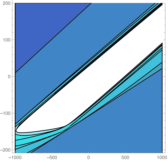
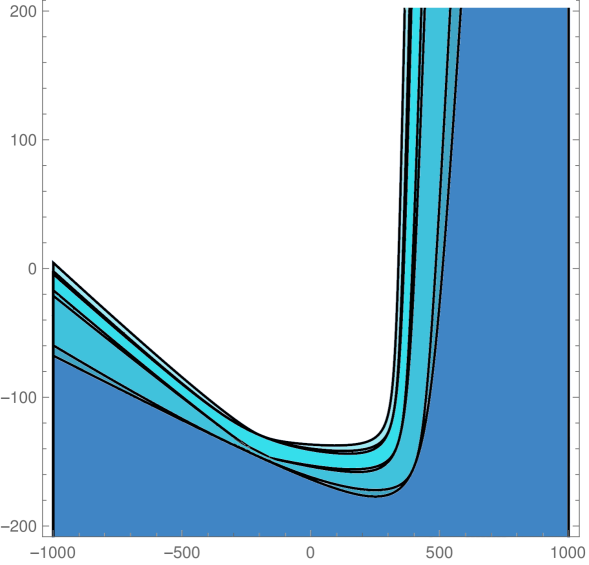
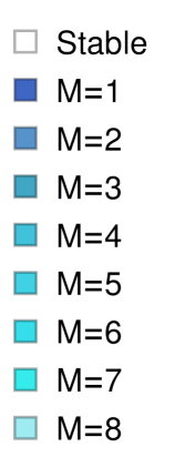
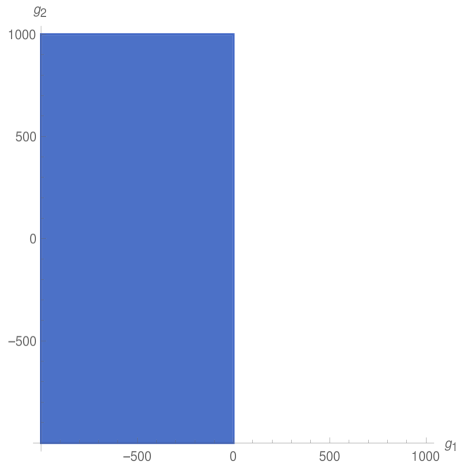
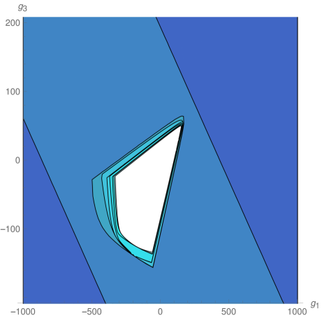
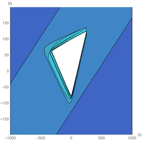
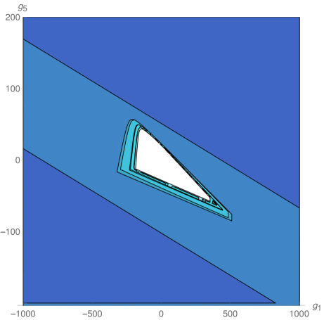
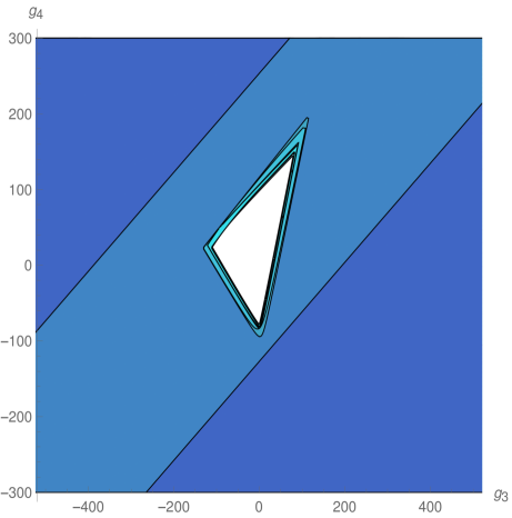
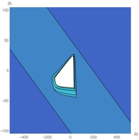
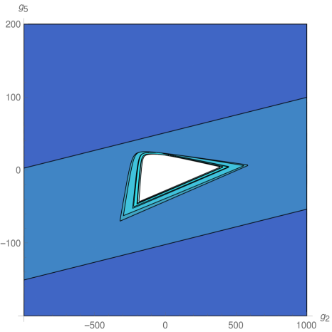
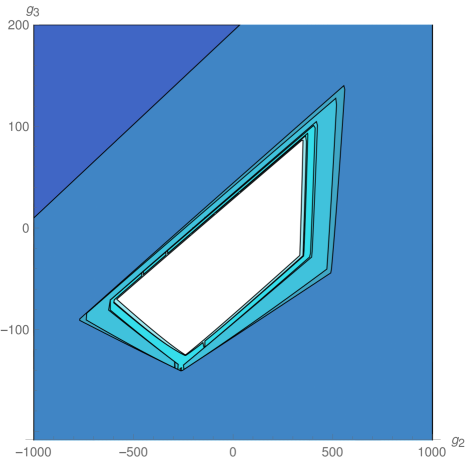
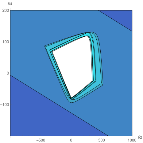
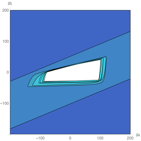
We explored the phase diagram by turning on the coupling constants by pairs. Sitting at different values of the non-vanishing couplings on every coupling plane, we evaluated the minors in equations (12) and (13) order by order. For example, on the plane -, we obtained the plots at the top of Fig.1. The regions are painted with a color that depends on the order of the first unstable minor. The plot on the top left correspond to instabilities that preserve rotational invariance, while that on the top right denotes instabilities that break it completely. These plots were combined on the one at the bottom. The resulting unstable regions of the phase diagram can be seen in Fig. 2, in which all different coupling planes are presented. We see that as grows (and so does the degree of the polynomial in point 4 above) the region in coupling space where the system is stable gets smaller, converging to an isolated wide island around the origin, which is simply connected.
In order to interpret our results from the boundary perspective, we recall that the electron star describes a holographic strongly coupled theory whose ground state has a fermionic condensate Hartnoll:2010gu . Classical spinor perturbations on the bulk then correspond to fermionic excitations on the boundary theory Hartnoll:2011dm .
The interesting point is that, as we decompose the bulk spinor into -modes, the set of Fermi momenta we obtained for them corresponds exactly to those defining the “holographically smeared Fermi surface” in reference Hartnoll:2011dm . It is natural then to interpret collective bulk modes, made by deforming the Fermi surface of each bulk mode, as corresponding to collective excited states on the boundary theory. These “deformations of the smeared Fermi surface” become unstable when a bulk Pomeranchuk instability shows up, leading to an instability of the boundary state that could easily be interpreted as a boundary Pomeranchuk instability.


6 Conclusions and outlook
We developed a general method to study anisotropic fermionic instabilities on a strongly coupled Fermi liquid via the AdS/CFT duality. It entails to perform a Pomeranchuk analysis on the dual bulk fermion, adapting the formalism to a curved space-time with a planar slice. The key step is to rewrite the single fermion in the bulk in terms of its modes in the holographic direction, resulting on a multi-component systems of lower dimensional fermions which move in the planar slice. By analyzing the minors of a quadratic form, we are able to detect when the fermionic modes become unstable under anisotropic deformations of their Fermi surface. The resulting phase transition breaks the rotational symmetry in the planar slice, and consequently in the boundary theory, potentially leading to a nematic phase.
We kept the formalism as general as possible, being suitable to be applied to many Euclidean-invariant boundary theories. This includes the zero temperature electron star Hartnoll:2010gu ; Hartnoll:2011dm , the finite temperature electron star Puletti:2010de ; Hartnoll:2010ik , as well as other examples222Since the method relays on the existence of a bulk Fermi surface, to adapt it to backgrounds such like the holographic metal Lee:2008xf ; Liu:2009dm ; Faulkner:2010da ; Faulkner:2009wj , the holographic superconductor Hartnoll_2008 , the magnetically charged black-hole Albash_2008 , or the Lifshitz geometry Kachru:2008yh , one would need to work in the limit in which a bulk fermion condensate would not backreact. This limit can be subtle, and it is hard to reconcile with the validity conditions for the WKB method, so the fermion wave functions should be solved using a different approximation.. We applied the method to the zero-temperature electron star background, being able to identify the unstable region on a five dimensional coupling space.
The method can be extended to more general situations relevant to condensed matter systems. Some examples of possible future directions are:
-
•
Finite doping: the inclusion of a doping axis should be straitforward, following the lines described in Kiritsis2016 .
-
•
Finite magnetic field: the inclusion of a magnetic field would require a magnetically charged background Albash_2008 333See footnote 2., and it would modify the bulk fermion coupling. Also, the Pomeranchuk analysis needs to be adapted dos .
-
•
Finite temperature fluid: as it stands, the method can be applied to the background of Puletti:2010de ; Hartnoll:2010ik in which the temperature is included via the presence of a horizon, while the bulk fluid is approximated as a finite temperature Fermi liquid. Including the effect of temperature in the bulk matter would modify the background, as well as the Pomeranchuk analysis uno .
-
•
Lifshitz scaling: considering Lifshitz geometries Kachru:2008yh would require a rewriting of the asymptotic conditions on the near boundary fermion, but the rest of the analysis remains mostly unchanged.
-
•
Lattice fermions: describing an underlying lattice in the holographic setup would imply the inclusion of a lattice-like metric Horowitz2012 or momentum relaxation Andrade2014 , and a modification of the Pomeranchuk analysis according to the lines of PhysRevB.78.115104 .
These are only some of the situations to which the method can be extended, we think that they deserve further investigation.
As a last remark, one could wonder whether Pomeranchuk instabilities are evident in physical quantities as we approach the edge of the unstable region444We would like to thank the referee for rising this point.. In a weakly coupled Fermi liquid, standard Landau theory arguments show that Landau parameters appear into some response functions. This happens for example for the compressibility or the spin susceptibility. The expressions are such that these functions become infinite when the instability is triggered by the correct Landau parameter.
Recalling that, according to Kubo formulae, response functions are written in terms of two-point correlators of local quantities, we can calculate them in holography. This is done by perturbing the background fields with the right IR boundary conditions and then evaluating the quotient of the leading and subleading parts of the perturbations at the UV. However, it is evident that in such calculation the fermionic couplings would only enter at higher loops. Since there is no reason to assume that bulk perturbation theory would break down close to the edge of the unstable region, the natural conclusion is that, in the strongly coupled boundary theory, the response functions are not sensitive to the instability.
Aknowledgements
The authors thank Pablo Rodríguez Ponte and Ignacio Salazar Landea for relevant contributions during the early stages of this work. We also thank Carlos Lamas for helpful comments. This work has been funded by the CONICET grants PIP-2017-1109, PIP-2015-0688 and PUE 084 “Búsqueda de Nueva Física”, and UNLP grants PID-X791, PID-11/X910.
Appendix A Fermionic states in a holographic background
In this Appendix, we work out a basis of free fermionic modes in a charged planar holographic background. We do so by writing the background in terms of vielbein and spin connection (section A.1), deriving the form of the corresponding Dirac equation (section A.2), separating it into spin components and Fourier modes in the planar and time directions (section A.2.1), and obtaining an effective Schrödinger equation that describes the fermion profile in the holographic direction (section A.2.2). We write the solution (section A.3) and notice that boundary conditions would generically imply a quantization of the frequencies as functions of the momenta (section A.3.1), resulting in a bunch of dimensional dispersion relations. We finally obtain the normalization constants, and check that with the so defined basis the resulting second quantized theory satisfy correctly normalized commutation relations (section A.3.1).
A.1 The background
We work with a generic planar asymptotically AdS charged background, with the form
| (14) | |||||
| (15) |
Here , and , and consequently and , are functions of . Since we want to couple fermions to the present background, we need the explicit form of the vielbein and dual vector basis that we wrote in the second equality. In terms of the planar indices , they read
| (16) |
This allows us to calculate the non-zero components of the spin connection by imposing metricity , and torsionless conditions. They take the form
| (17) | |||||
| (18) | |||||
| (19) |
This allows us to write the Dirac equation for a charged fermion in the present background, as we do in the next subsection.
A.2 The Dirac equation
A.2.1 Separation of variables and spin components
We consider a four-component Dirac spinor with charge under the gauge field coupled to gravity through the covariant derivative
| (20) |
where the Dirac gamma-matrices obey , and are the generators in the spinorial representation of the local Lorentz group in dimensions. We use along the paper the following representation for the gamma matrices
| (21) |
where are the Pauli matrices.
The free fermionic modes satisfy the Dirac equation
| (22) |
To solve it, we find convenient to work in momentum space
| (23) |
where , are the energy and momentum along the plane, is a normalization constant, and the factor has been included for later convenience. We can use rotational invariance to refer the momentum to the -axis, as
| (30) |
This allows us to write where
| (31) |
is the spinor representation of the rotation matrix (30), where is the identity matrix, and we used the explicit form of the generator . The resulting form of the equation (22) for now reads
| (32) |
Notice that this equation is real due to the choice of gamma matrices (21).
Let us now introduce the projectors
| (33) |
With their help we can decompose the Dirac field into “spin” states as , where the projected fields are
| (34) |
where each of the have two components. Inserting the resulting decomposition in (23), we obtain a solution with energy momentum and “spin” of the form
| (35) |
Plugging this back into the field equation (32) we get a decoupled system for the bi-spinors , as
| (36) |
This system can now be turned into a second order, Schrödinger-like equation for a single function , that is completely determined (up to normalization) by imposing smoothness at the boundary and smoolthness/ingoing boundary conditions at the horizon. We do this in the next subsection 555 It is worth to notice that from the representation (21) the generators of the Lorentz subgroup in dimensions are (37) From here it should be clear that are not Dirac spinors in dimensions, since they mix under Lorentz transformations. .
A.2.2 The effective Schrödinger equation.
We want to transform (36) into a second order Schrödinger equation to which we can apply our intuitions regarding wave functions. In order to do that, let us introduce the functions
| (38) |
Now, if we consider first , we can parameterize the bi-spinor in terms of two functions and , in the form
| (39) |
then substituting in (36) we get from its components the pair of coupled first order equations
| (40) | |||||
| (41) |
from the first of which we can rewrite
| (42) |
and now plugging this into the second equation, we get a second order Schrödinger-like equation for
| (43) |
where the potential is given by
| (44) |
If instead we consider , we can parametrize the bi-spinor in terms of the functions and , as
| (46) |
After introducing it in (36) we get as before a pair of coupled first order equations
| (47) | |||||
| (48) |
From the first equation we can obtain
| (49) |
and by plugging it into the second equation of (47) we get a second order Schrödinger-like equation for the function , with the form
| (50) |
with exactly the same potential (44) as before.
We look for solutions of (43) or equivalently (50) which do no diverge neither at the boundary nor at the horizon. In other words, we need normalizable solutions to the Schrödinger-like problem.
A last remark: we could try a solution of equations (36) such that: in (39) or (46). However, that would not be a smart choice since it would introduce a vanishing denominator at (42) or (49) whenever vanishes at negative value of the momenta. A better definition is to write (39) and (46) with the unique solution of (50), as we will show nextly.
A.3 General form of the free fermionic bases
A.3.1 Quantization of the frequencies
We must now impose boundary conditions on our solutions, in order to ensure smoothness everywhere. In particular, we impose regular boundary conditions in the ultraviolet, and we can chose either regular or in-going boundary conditions in the infrared.
The boundary conditions have an important consequence: the frequency is not free but is related to the modulus of the two-momentum through a dispersion relation that is in general labelled by some integer index , resulting in (see section F.2 for explicit forms of dispersion relations). This allows us to replace the indices in our functions of the previous sections by .
Taking into account these facts, and collecting the results given in (36)-(50) we can write for the fermionic mode in (35), the general form
| (58) |
where and are given in (42) and (49) respectively, in terms of the solution of (43) (or equivalently of (50)). Notice that the -tuple in parenthesis on the right corresponds to what was called in equation (35), and that will be referred bellow as in attention to the quantization of the frequencies.
A.3.2 Normalization
To completely define the modes (58) we need to fix their normalization. To this end we introduce in the space of spinors the following scalar product Birrell:1982ix
| (59) |
where is the space of constant and
| (60) |
is the induced metric on it. It is not difficult to prove that in the space of solutions to the Dirac equation (22) the operator is hermitian, i.e.
| (61) |
Standard arguments then show that eigenspinors of with different eigenvalues are orthogonal with respect to (59). By applying this result to the spinors (58) we know that they result orthogonal for different ’s. By using this fact we straightforwardly get the orthonormality relation
| (62) |
if the normalization constant is fixed such that
| (63) |
Finally, after the calculations above, the general solution of (22) can be written in coordinates space as
| (64) |
For later use, it is worth to remind that (62) yields for the above solutions the completeness relation
| (65) |
As we will see in the next section, the above defined normalization provides canonical anti-commutation relations for the corresponding Hamiltonian variables. This allows us to define canonical creation and annihilation operators for the fermionic modes in the bulk. With this, we will be able to establish a standard Landau description for the bulk Fermi liquid.
Appendix B Hamiltonian theory
In this Appendix we develop the Hamiltonian theory for the fermions in the bulk, using the orthonormal basis obtained in the previous section. In section B.1, we define our dynamics for the fermionic degrees of freedom, and write the generic form of the corresponding Hamiltonian. Then in section B.2 we deal with its free part, while the interacting part is worked out in section B.3.
B.1 Dynamical setup
The action for our spinor field that propagates in the asymptotically AdS bulk reads
| (66) |
where the ’s are spin indices running from to , and we have defined the conjugate spinor . We included a four-fermion interaction term, which takes the most general form that respects covariance in four-dimensional curved space and fermion number conservation. It is written in terms of an invariant tensor given by
| (67) | |||||
| (68) |
where we defined . This tensor satisfies the condition , as well as the Lorentz invariance property
| (69) |
for any Lorentz transformation , where denotes its spinorial representation. This property will be useful in what follows, in particular when we apply it to the rotation on the plane represented by the unitary matrix defined in (31).
From the action (66) the momentum conjugate to the spinor field is
| (70) |
allowing us to write the Hamiltonian as
| (71) |
where can be read from (66).
Inserting the momentum (70) into the canonical anti-commutation relations for coordinates and momenta, we get that the spinor field satisfies
| (72) |
Then from the decomposition (64) we get the standard anti-commutation relations
| (73) |
identifying and as the creation and annihilation operators respectively for the fermionic modes in the bulk. In the rest of this section we rewrite the bulk dynamics given by (71) in terms of them.
B.2 The free Hamiltonian
Let us first take the free part of the Hamiltonian (71), which reads
| (74) |
now using the Dirac equation we get
| (76) |
Then inserting the decomposition (64) and using the orthogonality relation (65) we get the free Hamiltonian in terms of creation and annihilation operators, as
| (77) |
In other words, the bulk degrees of freedom are described by a set of independent fermionic species labelled with an integer index corresponding to the mode on the direction. Each species has a dispersion relation given by , with a two-fold degeneracy given by the spin .
B.3 The interaction Hamiltonian
Regarding the interacting part of the Hamiltonian, we have
| (78) |
Plugging the decomposition (64) into (78) we get
where the integral has been performed explicitly giving origin to the momentum conservation -function, while the integral is contained in the definition of the momentum-space interaction tensor
in terms of the integrals
| (81) |
where functions are defined as in equation (35) and correspond to the -tuples in parenthesis on the right of equation (58). As we show below, only a subset of the integrals (LABEL:eq:fermion.integrals.all) is needed for a Landau description of the bulk fluid.
Appendix C Landau description of the bulk fermions
In the previous section we rewrite the dynamics of the Dirac spinor in the bulk as that of a bunch of fermionic species in one less dimension, indexed by the energy mode and the spin . In the present appendix, we develop a description in terms of the Landau theory for a multi-component Fermi liquid. We do that by using a perturbative approach.
C.1 Perturbative derivation
We work in the grand canonical ensemble at chemical potential and temperature (that we will take to zero at the end of the calculations). We define the expectation value of an operator by
| (83) |
where is the number of particles and is the grand canonical potential. The last formula can be inverted according to
| (84) |
To perform a perturbative approximation, we write the Hamiltonian as
| (85) |
and assume that the constants in (67) are small. With the help of the free Hamiltonian we define the zeroth order quantities
| (86) |
Then expanding (83) to first order in , we obtain
| (87) |
which implies for the grand canonical potential
| (88) |
For the first term in (88) we can write
| (89) |
where are the occupation numbers of the one-particle states . This implies for the free part of the grand canonical potential
| (90) |
On the other hand, to write the second term in (88), we use (B.3) to have
| (91) |
Calculating the expectation value in the right hand side
| (92) | |||
we replace back in (91) to get
| (93) |
where the “Landau interaction functions” are defined according to
| (94) |
Here we used the definition (B.3), and re-absorbed into the couplings an infinite constant coming from collapsing the momentum integrals666Formally this is accomplished by regularizing through the introduction of a finite volume in coordinate space, and then taking the infinite volume limit at the end of the calculations.. The Landau interaction functions contain all the information about the interactions on the multi-component Fermi liquid. They verify the following relations
| (95) |
At this point of the discussion, a remark is in order. It is usual for condense matter theorists to think about the Landau interaction function as a correlation function. More precisely, let us introduce the index and denote by
| (96) |
the one-particle irreducible vertex that describes the interacction of two elementary excitations. Then it can be shown that 777 As they are not essential for the argument, we do not care here with numerical factors and propagators residues, that in any case are irrelevant in the order at which we work, see nozieresdupuis for details.
| (97) |
At leading order in perturbation theory the right hand side of (96) reads peskin
| (98) | |||||
| (99) |
where in the first line all the operators are in the interaction picture, with the interacting Hamiltonian given in (B.3), and in the second line we omitted a momentum conservation delta-function. By plugging (98) into (97) we get our result (94).
A perturbation of the ground state occupation numbers gives us a variation of the grand canonical potential with the form
| (101) |
where the quasiparticle dispersion relation has been defined as
| (102) |
For any perturbation the quantity must be positive to have a stable ground state. Whenever it becomes negative, an instability is triggered.
C.2 Explicit form of the Landau interaction functions
We want to obtain a more explicit form of the Landau interaction functions suitable of being implemented into a numerical code. The integrals (LABEL:eq:fermion.integrals.all) we need are
| (103) |
and they satify what can be used to rewrite (B.3) as
| (104) | |||||
| (105) |
To further disentangle the angle dependence, we find convenient to use the explicit form of the spinorial rotations matrices (31) to write
| (106) |
where the constant, cosine and sine auxiliary tensors are given respectively as
| (107) | |||||
| (108) | |||||
| (109) |
By inserting this expressions into (104)-(105) we finally obtain from (94) a completely factorized form for the Landau interaction functions, as
| (110) |
written in terms of three independent constant, cosine and sine components, which are given according to
| (111) | |||||
| (113) | |||||
| (115) | |||||
| (117) | |||||
| (119) | |||||
| (121) |
Notice that we dropped any auxiliary quantity, having obtained a formula for the Landau interaction functions which is completely written in terms of the interaction tensor (67) and the integrals (103) of the form (LABEL:eq:fermion.integrals.all), where the radial functions were defined in equations (35)-(58) in terms of the solutions of equation (50).
Appendix D Pomeranchuk method
We give in this section a brief introduction to Pomeranchuk’s method to detect instabilities in a Landau fermi liquid. We focus on the isotropic, two dimensional case, since it is what concern us in this paper. We begin by explaining the method for a single spinless fermion (section D.1), the generalization for multiple species of spinful fermions is given later (section D.2).
D.1 Single spinless fermion
Given a two-dimensional system of spinless fermion with quasiparticle dispersion relation , its Fermi surface is defined in momentum space by the relation . In the ground state all the single quasiparticle states with momenta are occupied, while those with momenta are empty. In other words, we can write the occupation number as , where is the Heavyside step function.
A fermionic excitation can then be represented by a small deformation of the Fermi surface, charactherized by a variation of the occupation numbers . The excitation energy at weak coupling is then given by Landau’s formula (101)
| (122) |
where is the Landau interaction function. The variation on the occupation numbers of the state take the values at any point with of momentum space. They can be parametrized as
| (123) |
where is an auxiliary function that characterizes the deformation of the Fermi surface. By using the expansion of the Heavyside function in terms of Dirac delta function and its derivatives, we get888This is a shorthand calculation, if the reader is uncomfortable with it, (124) can be smoothed by making the replacement and then taking the limit.
| (124) |
When replacing (124) into (122), the Dirac delta functions enforce the integrands to be evaluated at , namely at the Fermi surface. Using polar coordinates in momentum space, this implies that the integrand must be evaluated at and then the momentum integrals reduce to angular ones
| (125) |
where by using rotational invariance we wrote and . Here the Fermi velocity is defined as .
A Fourier expansion now allows us to write
| (126) |
and similarly, to parameterize the deformations by the amplitudes in the decomposition
| (127) |
Replacing (126) and (127) in (125) we obtain:
| (128) |
We see that the excitation energy ends up written as a quadratic form in the deformation amplitudes . In order to have a stable system, has to be positive for any possible excitation, or in other words for any possible amplitudes. This implies that the above defined quadratic form must be positive definite, leading to the stability conditions:
| (129) | |||||
| (130) |
If any of these conditions is violated, the system becomes unstable. Notice that the parameters completely disappear from the calculation. The parameters are called the “Landau parameters” of the Fermi liquid.
It is important to stress that, when working in perturbation theory, the dispersion relation is defined by (102) as
| (131) |
This implies that only the zeroth order forms of the Fermi momentum and Fermi velocity have to be kept in equations (129). Indeed, since the second term in those inequalities contains a Landau parameter , it is already first order in the coupling constants. Thus we can replace (129) by
| (132) | |||||
| (133) |
where is obtained from and we defined .
D.2 Multiple fermionic species with spin
The above procedure can be easily generalized to many species of spinful fermions, the resulting quadratic form being in general non-diagonal in the indices denoting spin and species . As we know, the excitation energy of such fermionic system is given by (101)
| (134) |
When the deformations of the occupation numbers get spin and species indices , so do the functions parameterizing the deformations
| (135) |
Notice that each species and spin component has its own Fermi momentum at which it dispersion relation vanishes . Going through the same steps as before we get for the energy fluctuation
| (136) |
where and .
Now we must decompose the interaction function as in (126)
| (137) |
Although from (110) we can already see that in our case only the modes are present in the decomposition (137), we mantain the general analysis for now. The deformation parameters can be decomposed in parallel with (127) to get
| (138) |
in terms of the deformation amplitudes .
Going ahead to plug the decompositions (137) and (138) into (136), we get the generalization of (128) to be
| (141) | |||||
On a stable state, this quadratic form has to be positive definite. Neccesary and sufficient conditions for stability can be obtained by considering the following two disantangled cases.
-
•
Putting and for , we have that the first line in (141) must be positive definite, that applying Sylvester’s criterion is equivalent to,
, (142) where stands for the -th minor, that is the determinant of the upper-left submatrix.
-
•
Considering now the opposite case: and for , we have to impose the positivity of the quadratic form: defined by the second and third lines in (141) for each separetely, since they do not couple. To simplify the analysis, we find convenient to introduce the perturbation vectors in indices : and . Then we can write,
(143) where the matrices and are read from (141). By further defining the complex vectors , (143) takes the simple form
(144) From here it is clear that the positivity condition of is just that the hermitian matrices must be positive, for any . By using the explicit expressions of and , this is equivalent to ask that
(145)
In conclusion, if any of the minors in (142) and (145) is negative, the quadratic form has a negative mode that would lead to an excitation with negative energy: , thus triggering an instability on the fermionic system.
D.3 Summary and application to the holographic setup
In summary, in order to perform the stability analysis, all we need are
- •
- •
-
•
The Fourier components of the Landau parameters, evaluated at the free Fermi momenta . Notice that equation (110) implies that only the modes with enter into the stability analysis in the holographic setup. The Landau parameters are obtained from (111) in terms of the integrals (103) evaluated at the free Fermi momenta. Since , we need only static wave functions in (103).
Appendix E The electron star background
In this appendix, we summarize the construction of the electron star solution. We do so in order to fix notation and to have a fully self-contained discussion. However, all the results presented in this section were obtained in the original reference Hartnoll:2010gu to which the interest reader is referred.
We work with the previously presented Ansatz (14)
| (146) | |||||
| (147) |
The field equations of -dimensional Einstein-Maxwell theory in the presence of a negative cosmological constant plus matter in the form of a charged perfect fluid are
| (148) | |||||
| (149) |
with and the gravitational and electromagnetic couplings respectively. Here the contributions to the energy-momentum tensor and current density read
| (150) | |||||
| (151) | |||||
| (152) |
The functions , and are the pressure, energy density and charge density of the fluid, respectively, and its four-velocity. Furthermore, the conservation equations must hold
| (153) |
Since we aim to describe a relativistic system of fermions of mass , we can try a description of the energy and charge densities in terms of the density of states in flat space of a free fermion gas . This description would be accurate as long as the wavelength of the fermions is much shorter than the local curvature radius. Furthermore, we must consider the equation of state of the system in terms of a grand canonical potential . At zero temperature the fluid functions read
| (154) | |||||
| (155) | |||||
| (156) |
where is the bulk Fermi energy. Consistency with Ansatz (146) imposes that all the functions be dependent only on . Moreover, the velocity of the fluid must be unitary, which identifies it with the vierbein temporal vector, i.e. , see (16). This last fact implies that the bulk Fermi energy coincides with the local (i.e. measured by comoving observers) chemical potential .
It is convenient to work with the dimensionless quantities
| (157) |
Here we introduced . In terms of these scaled variables (154) can be integrated to obtain the explicit expressions
| (158) | |||||
| (159) | |||||
| (160) |
where we introduced the two independent parameters and that can be used to define the electron star
| (161) |
By plugging (146) and (158) in (148) we get the field equations
| (162) | |||||
| (163) | |||||
| (164) |
These equations have to be solved numerically for each value of and to obtain the metric and gauge functions .
Regarding the boundary conditions in the IR, we observe from (158) that the electron star extends from infinity to the radius such that
| (165) |
whose position is determined by the equation
| (166) |
Outside the electron star, i.e. , we have that , implying that the equations of motion (162) reduce to
| (167) |
whose general solution is the AdS Reissner-Nördstrom black hole
| (168) |
To specify this solution we have to give the four integration constants. . In the electron star context they must be obtained by matching at the radius with the solution inside the star.
On the other hand, in the IR limit the solution acquires the form of a Lifshitz metric. In fact, an Ansatz for large of the form:
| (169) |
solves (162) if takes some of the following three values
| (170) |
The parameter is called the dynamical critical exponent. One can show that an IR non-singular, asymptotically exact Lifshitz solution exists only if
| (171) |
and the root selected is the negative one: , see Hartnoll:2010gu for details. From the leading order of (162) we get,
| (172) | |||||
| (173) | |||||
| (174) |
The first two equations determine the coefficients that define the Lifshitz metric in terms of and , while that the last equation relates implicitly in terms of and also. So it is possible, and convenient to make numerics, to think the Lifshitz parameter and the mass as the free parameters of the electron star. The expansions (169) result completely determined by (), and by that remains free. However, the scalings leave the Ansatz (146) invariant and induce the invariance of the system (162) under
| , | (175) | ||||
| , | (176) |
These scalings allow to fix the leading order term of in (169) together with the absolute value of , while the sign to get the solution with the right behaviour in the UV results to be the negative one. In the paper we work out the electron star solution by fixing .
In figure 3 we present the electron star background solution obtained after solving numerically the system (162). We can see how the electron star solution matches the AdS-RN and Lifshitz solutions in the UV () and IR () respectively.
An important point to be stressed is that, in the weak gravity regime both and conditions should hold, or what is the same, and . On the other hand, in Hartnoll:2010gu was shown that the flat treatment (158) is consistent only if we restrict the electron star parameters to the region . Together with the weak gravity conditions, they imply that
| (177) |
We will see in appendix F that these conditions are closely linked to the validity of the WKB approximation for the fermionic perturbations.
Appendix F The WKB solution
In the electron star background, we are assuming that we have a large number of particles inside one AdS radius. This is equivalent to the statement that the particle wavelength is much shorter than the characteristic length of the background in which it is moving. This implies that we can solve the effective Schrödinger equation (43) (or equivalently (50)) in the Wentzel-Kramers-Brillouin (WKB) approximation, as we do in the rest of this section.
F.1 Basics of the WKB approximation
Let us remember basic facts about the WKB approximation (see for example merzbacher1998quantum ). Let us consider the one-dimensional Schrödinger equation written in the form
| (178) |
We will assume that the potential is repulsive and positive at the boundary, implying that at close enough to we have and . As we move into positive values of we have a first turning point at which and . At larger values of additional turning points appear at which .
Away from any given turning point, we introduce the functions
| (179) |
As can be checked by direct substitution, they are good approximate solutions of (178) as long as is large enough, which means in particular that we can use them away from the turning points. On the other hand, close to any turning point we can linearize the potential, and the solution is then written in terms of Airy functions and . Then the WKB approximate solution around takes the form
| (185) |
where and are numerical constants to be determined in order to ensure the boundary conditions and the continuity around each turning point.
The coefficients of the functions at left and right of a given turning point are linearly related, as in
| (186) |
where the explicit form of the matrix is obtained by matching the functions across the turning point using the intermediate Airy form of the solution. It has the expression when , and when , with
| (187) |
The relation between the approximate WKB solutions around any pair of successive turning points can be found by shifting the limits of integration in (179) from to
| (188) |
in terms of the connection coefficients , which read
| (189) |
Compatibility with the form (185) for the solution around each turning point thus implies the additional linear relation
| (190) |
in terms of the connection matrix
| (191) |
With all the above, we can express the whole set of coefficients of the solution around each of the turning points, in terms of and , as follows
| (196) | |||||
| (201) | |||||
From this, we can write the relation between the initial (leftmost) and final (rightmost) coefficients for a system with a total of turning points. It takes the form
| (202) |
where
| (203) |
In the present context, Bohr-Sommerfeld quantization relations arise when we impose boundary conditions at both extremes of the axis. This leads to constraints on the matrix elements of and consequently on the parameters of the theory.
F.2 Application to the electron star background
After the re-scalings , together with (157) and (161), the potential (44) entering into the effective Schrödinger equation acquires the following form
| (204) |
As we will be working in an electron star background, we have to consider the large limit. From (204) we then see that this regime coincides with the semiclassical limit where the WKB approximation is reliable. In such limit we can neglect the last two terms in (204) and consider
| (206) |
Close to the AdS boundary , we can replace the functions and by their corresponding UV expansions (168), obtaining . This implies that the potential diverges at the boundary. Since the resulting function in (179) diverges as we move into the boundary , in order to have a normalizable solution, we need to impose .
In the deep IR, the functions take their Lifshitz form (169), and we get . In consequence, for zero frequency the potential goes to a positive constant at infinity. The corresponding function diverging, we need to impose . Combined with the conditions at the boundary we obtain or in other words
| (207) |
where the matrix element was defined in (203) in terms of integrals involving the potential . For finite frequency on the other hand, the potential diverges into negative values. This results in an with the form of a wave moving into smaller values, i.e. entering the bulk from infinity, which implies that we must impose in order to avoid causality issues. Since this implies
| (208) |
Equations (207) and (208) impose a constraint between the parameters entering into . It often has a discrete set of solutions, being then understood as a quantization condition (see below).
According to the summary on section D.3, using this information we need to obtain the free Fermi momentum and Fermi velocity for each mode in the direction, as well as its static wave function or in other words the solution of the effective Schrödinger equation (43) with and .
F.2.1 Fermi momenta and static wave functions
Of particular interest to our problem are the Fermi momenta, i.e. the values of the momentum satisfying . This implies that the corresponding potential in (206) has a vanishing frequency, and then goes to a positive constant at infinity. In consequence it has none or an even number of turning points.
The two last terms in the parenthesis in (206) are positive outside the star, and negative inside it, according to the rule (166). This implies that for large enough, the parenthesis remains always positive and there are no turning points. On the other hand, for smaller than some critical value , the potential becomes negative somewhere inside the star, giving rise to a pair of turning points . Only in this last case we are able to find values of the free Fermi momenta, all of them inside a “Fermi ball” Lee:2008xf of radius .
The connection matrix (203) has only three factors and the relevant matrix element in equation (207) takes the form
| (209) |
implying that the Bohr-Sommerfeld condition (207) reads
| (210) |
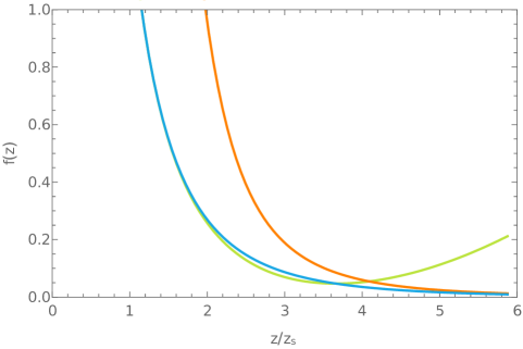
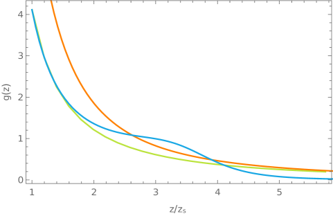
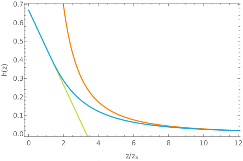
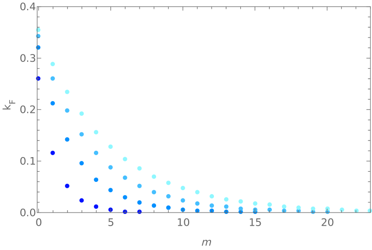
In terms of an integer , this equation determines the free Fermi momentum of the -th fermionic mode. The results of these calculations are shown in Fig. 4
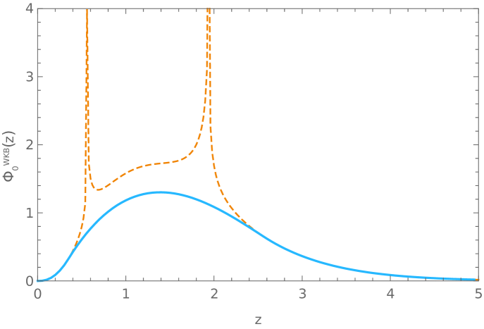
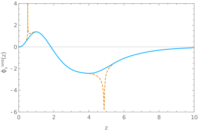
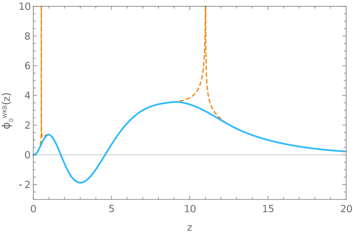
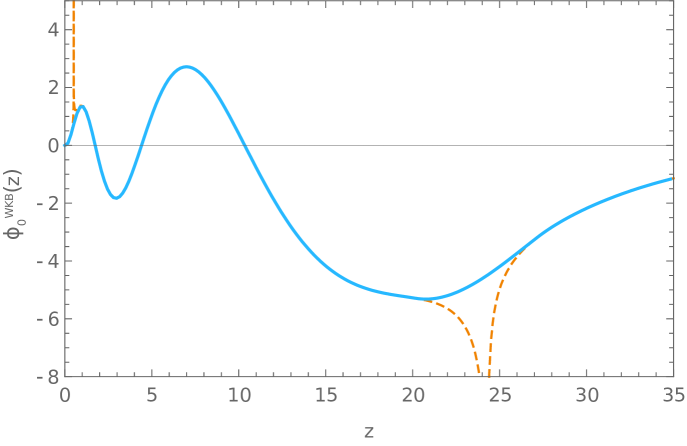
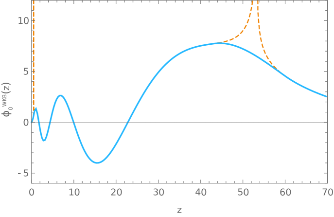
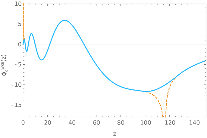
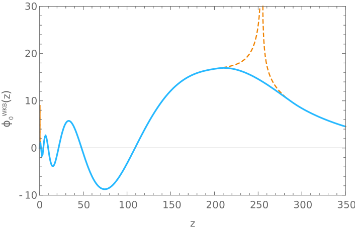
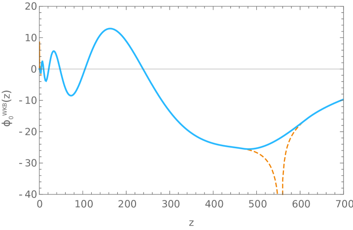
Next, we can replace the obtained values of the free Fermi momenta into equations (179)-(191) to obtain the corresponding solutions of (43) needed to build the static wave-functions. In our calculations we found useful to replace the Airy functions interpolating around the turning points in (185) by a quartic polynomial. Results are shown in Fig. 5.
F.2.2 Fermi velocities
To calculate the Fermi velocities , we need to concentrate in low energy excitations, with momenta very near to the Fermi momentum . This would result into small frequencies . As discussed previously, for any non-zero frequency the potential has an odd number of turning points. As our frequency is very small, along with the two turning points of the zero frequency case , only a third one appears. As goes to zero, the third turning point moves to infinity.
In this case the resulting connection matrix in (203) has the five factors , and (208) reads
| (211) |
The solution for the dispersion relation is necessarily complex, defining a problem of quasi-normal modes. Since the integral in the exponent of the right hand side of (211) diverges as goes to zero, the right hand side is very small. This implies that we can write (211) as
| (212) |
To the first order in and , we get
| (213) |
implying for the Fermi velocity
| (214) |
where the potential and the turning points are evaluated at zero frequency and .
In is worth to mention that a possible obstacle to get straight the dispersion relation at leading order from (212) arises from the non-analyticity of the complex right hand side of (211). However, as shown in Hartnoll:2011dm , it only affects (in fact, determines!) the imaginary part of the dispersion relation, while the real part is given as usual by the analytical left hand side.
References
- (1) S. Sachdev, Quantum Phase Transitions, Cambridge University Press (2000), 10.1017/CBO9780511622540.
- (2) G.R. Stewart, Non-fermi-liquid behavior in - and -electron metals, Rev. Mod. Phys. 73 (2001) 797.
- (3) I.Y. Pomeranchuk, On the stability of a fermi liquid, Sov.Phys.JETP 8 (1958) .
- (4) C.A. Lamas, D.C. Cabra and N. Grandi, Fermi liquid instabilities in two-dimensional lattice models, Phys. Rev. B 78 (2008) 115104.
- (5) C.A. Lamas, D.C. Cabra and N. Grandi, Generalized pomeranchuk instabilities in graphene, Phys. Rev. B 80 (2009) 075108.
- (6) C.A. Lamas, D.C. Cabra and N.E. Grandi, Pomeranchuk instabilities in multicomponent lattice systems at finite temperature, International Journal of Modern Physics B 25 (2011) 3539 [https://doi.org/10.1142/S0217979211102046].
- (7) P.R. Ponte, D.C. Cabra and N. Grandi, Reentrant behavior in landau–fermi liquids with spin-split pomeranchuk instabilities, Modern Physics Letters B 26 (2012) 1250125 [https://doi.org/10.1142/S0217984912501254].
- (8) P. Rodríguez Ponte, D. Cabra and N. Grandi, Fermi surface instabilities at finite temperature, The European Physical Journal B 86 (2013) 85.
- (9) O. Aharony, S.S. Gubser, J. Maldacena, H. Ooguri and Y. Oz, Large n field theories, string theory and gravity, Physics Reports 323 (2000) 183 .
- (10) S.-S. Lee, A Non-Fermi Liquid from a Charged Black Hole: A Critical Fermi Ball, Phys. Rev. D79 (2009) 086006 [0809.3402].
- (11) H. Liu, J. McGreevy and D. Vegh, Non-Fermi liquids from holography, Phys. Rev. D83 (2011) 065029 [0903.2477].
- (12) T. Faulkner, H. Liu, J. McGreevy and D. Vegh, Emergent quantum criticality, Fermi surfaces, and AdS(2), Phys. Rev. D83 (2011) 125002 [0907.2694].
- (13) T. Faulkner, N. Iqbal, H. Liu, J. McGreevy and D. Vegh, From Black Holes to Strange Metals, 1003.1728.
- (14) S.A. Hartnoll and A. Tavanfar, Electron stars for holographic metallic criticality, Phys. Rev. D83 (2011) 046003 [1008.2828].
- (15) S.A. Hartnoll, D.M. Hofman and D. Vegh, Stellar spectroscopy: Fermions and holographic Lifshitz criticality, JHEP 08 (2011) 096 [1105.3197].
- (16) M. Cubrovic, Y. Liu, K. Schalm, Y. W. Sun and J. Zaanen, Phys. Rev. D 84 (2011), 086002 doi:10.1103/PhysRevD.84.086002 [arXiv:1106.1798 [hep-th]].
- (17) M. Edalati, K.W. Lo and P.W. Phillips, Pomeranchuk Instability in a non-Fermi Liquid from Holography, Phys. Rev. D 86 (2012) 086003 [1203.3205].
- (18) Y. Liu, K. Schalm, Y. W. Sun and J. Zaanen, JHEP 05 (2014), 122 doi:10.1007/JHEP05(2014)122 [arXiv:1404.0571 [hep-th]].
- (19) S.A. Hartnoll, C.P. Herzog and G.T. Horowitz, Holographic superconductors, Journal of High Energy Physics 2008 (2008) 015–015.
- (20) V.G.M. Puletti, S. Nowling, L. Thorlacius and T. Zingg, Holographic metals at finite temperature, JHEP 01 (2011) 117 [1011.6261].
- (21) S.A. Hartnoll and P. Petrov, Electron star birth: A continuous phase transition at nonzero density, Phys. Rev. Lett. 106 (2011) 121601 [1011.6469].
- (22) K. Capelle and E.K.U. Gross, Relativistic framework for microscopic theories of superconductivity. i. the dirac equation for superconductors, Phys. Rev. B 59 (1999) 7140.
- (23) E. Kiritsis and L. Li, Holographic competition of phases and superconductivity, Journal of High Energy Physics 2016 (2016) 147.
- (24) T. Albash and C.V. Johnson, A holographic superconductor in an external magnetic field, Journal of High Energy Physics 2008 (2008) 121.
- (25) S. Kachru, X. Liu and M. Mulligan, Gravity duals of Lifshitz-like fixed points, Phys. Rev. D78 (2008) 106005 [0808.1725].
- (26) G.T. Horowitz, J.E. Santos and D. Tong, Optical conductivity with holographic lattices, Journal of High Energy Physics 2012 (2012) 168.
- (27) T. Andrade and B. Withers, A simple holographic model of momentum relaxation, Journal of High Energy Physics 2014 (2014) 101.
- (28) N. Birrell and P. Davies, Quantum Fields in Curved Space, Cambridge Monographs on Mathematical Physics, Cambridge Univ. Press, Cambridge, UK (2, 1984), 10.1017/CBO9780511622632.
- (29) E. Merzbacher, Quantum Mechanics, Wiley (1998). ISBN-13: 978-0471887027, ISBN-10: 0471887021
- (30) P. Nozières, Theory of interacting Fermi systems, Avalon Publishing (1997); N. Dupuis, Fermi liquid theory, lecture notes at Laboratoire de Physique des Solides, Universitè Paris-Sud, Orsay, France (2019).
- (31) M. Peskin and D. Schroeder, An Introduction To Quantum Field Theory, Avalon Publishing, (1995);