Pop-Stack Operators for Torsion Classes and Cambrian Lattices
Abstract.
The pop-stack operator of a finite lattice is the map that sends each element to the meet of , where is the set of elements covered by in . We study several properties of the pop-stack operator of , the lattice of torsion classes of a -tilting finite algebra over a field . We describe the pop-stack operator in terms of certain mutations of 2-term simple-minded collections. This allows us to describe preimages of a given torsion class under the pop-stack operator.
We then specialize our attention to Cambrian lattices of a finite irreducible Coxeter group . Using tools from representation theory, we provide simple Coxeter-theoretic and lattice-theoretic descriptions of the image of the pop-stack operator of a Cambrian lattice (which can be stated without representation theory). When specialized to a bipartite Cambrian lattice of type A, this result settles a conjecture of Choi and Sun. We also settle a related enumerative conjecture of Defant and Williams. When is an arbitrary lattice quotient of the weak order on , we prove that the maximum size of a forward orbit under the pop-stack operator of is at most the Coxeter number of ; when is a Cambrian lattice, we provide an explicit construction to show that this maximum forward orbit size is actually equal to the Coxeter number.
1. Introduction
1.1. Pop-stack
Let be a finite lattice with meet operation and join operation . The pop-stack operator and the dual pop-stack operator are defined by
where we write to mean that is covered by in . These operators have appeared in various contexts; they serve as both useful tools [AP22, BH, Eno23, ES22, Hana, Müh19, Rea11, Sak] and objects of interest in their own right [CS, CG19, CGP21, Def22b, Def22a, DW23, Hon22, PS19, Ung82]. When the lattice is understood, we will omit subscripts and simply denote these operators by and .
In [CG19, Def22b, Def22a, Hon22, PS19, Ung82], the pop-stack operator has been considered as a dynamical system. Given a map and an element , the forward orbit of under is the set
where is the map obtained by composing with itself times. To ease notation, let us write
for the forward orbit of under . If is sufficiently large, then is equal to the minimal element of (which is a fixed point of ). Thus, is equal to the number of iterations of needed to send to . Given an interesting lattice , one of the primary problems one can consider about its pop-stack operator is that of computing
For a fixed , one can also consider the -pop-stack sortable elements of , which are the elements such that .
Defant and Williams [DW23] also found that it is fruitful to study the image of the pop-stack operator when is a semidistrim lattice; this is because the image of has numerous interesting properties, some of which relate to a certain bijective rowmotion operator . For example, and are both equal to the number of elements such that . The images of and are also naturally in bijection with the set of facets of a certain simplicial complex called the canonical join complex of .
1.2. Lattices of torsion classes
In this article, we take a representation-theoretic perspective and consider a finite-dimensional basic algebra over a field . The set of torsion classes (see Section 3.2 for the definition) of finitely-generated (right) -modules forms a complete lattice [IRTT15] that we denote by . Examples of lattices arising in this way include the weak order and Cambrian lattices associated to any finite crystallographic Coxeter group [AHI+, Miz14, IT09]. This paper continues a rich tradition of using lattices of torsion classes as a tool for proving new results in both representation theory and in algebraic combinatorics; see, e.g., [DIR+23, Eno23, IRRT18, RST21, TW19b, TW19a] and many others.
We focus our attention on the case when is -tilting finite (in the sense of [DIJ17]); this is equivalent to assuming is finite. Our goal is to study the image and the dynamical properties of the pop-stack operator of . While has already appeared (sometimes under different names) in the theory of lattices of torsion classes [AP22, BH, Eno23, ES22, Hana, Sak], it has primarily been used as a tool rather than a dynamical operator worthy of its own investigation. Let us remark that the article [BTZ21] initiated the study of dynamical combinatorics of torsion classes by considering rowmotion.
In Section 4, we consider certain pairs of sets of modules called 2-term simple-minded collections and semibrick pairs. 2-term simple-minded collections were first introduced in the special case when is a symmetric algebra in [Ric02]; they are special cases of the more general simple-minded collections introduced in [AN09] (under the name spherical collections). Semibrick pairs are a generalization of 2-term simple-minded collections that were introduced in [HI21b] as a tool for studying a generalization of the picture group of [ITW]. As we recall in Section 3.3, there is a bijection between (with -tilting finite) and the set of 2-term simple-minded collections [Asa20]. By the results of [BCZ19], this bijection encodes information about cover relations and canonical join representations in .
The set also comes equipped with a set of mutation operators that categorify the mutation theory of cluster algebras. See [BY13, Section 3.7] and [KY14, Section 7.2] (special cases also appeared earlier in [KS, Section 8.1] and [KQ15, Section 3]). These mutation formulas can also be applied to many of the more general semibrick pairs; see [BH22, HI21a]. Moreover, under the bijection between and , the mutation operators give a representation-theoretic formula for how the corresponding 2-term simple-minded collection changes when one traverses a cover relation in .
For each semibrick pair , there is classically one mutation operator for each module in . In the present paper, we more generally define a mutation operator for each nonempty subset or . Our first main result (Theorem 5.1) states that, under the bijection between and , applying the pop-stack operator and its dual to a torsion class corresponds to performing certain mutations on the associated 2-term simple-minded collections.
In Section 5.2, we characterize the preimages of a prescribed torsion class under and . As corollaries, we obtain descriptions of the -pop-stack sortable and the -pop-stack sortable elements of (Corollaries 5.4 and 5.5).
1.3. Cambrian lattices
Let be a finite irreducible Coxeter group, and let denote the (right) weak order on . Given a Coxeter element of , one can construct the -Cambrian lattice , which is the sublattice of consisting of Reading’s -sortable elements [Rea06, Rea07]. (The -Cambrian lattice is also a lattice quotient of .) When is crystallographic, we can realize as the lattice of torsion classes of the tensor algebra associated to the weighted Dynkin quiver associated to [IT09].
Two very special Cambrian lattices are the Tamari lattice and the type-B Tamari lattice; the images of the pop-stack operators on these lattices were characterized and enumerated in [Hon22] and [CS], respectively. On the other hand, analogous results for the Cambrian lattice associated to a type-A bipartite Coxeter element have remained elusive: a conjectural enumeration of the image was formulated by Defant and Williams [DW23], while a characterization of the image was conjectured by Choi and Sun [CS].
It turns out that our representation-theoretic perspective is quite useful for understanding the image of . In Theorem 5.10, we provide a representation-theoretic characterization of the image of whenever is hereditary. When the Coxeter group is crystallographic, the tensor algebra is hereditary, and we can reformulate our description of the image of the pop-stack operator in purely lattice-theoretic and Coxeter-theoretic terms. We then check directly (by hand and by computer) that these lattice-theoretic and Coxeter-theoretic descriptions still holds when is not crystallographic.
Our Coxeter-theoretic description of the image of is surprisingly simple: we will prove (Theorem 7.8) that a -sortable element is in the image of if and only if the right descents of all commute and has no left inversions in common with .
To state our purely lattice-theoretic description of the image of , let us write for the simple reflections of ; these are the atoms of . For , let be the unique maximal element of the set
We will prove that an element is in the image of if and only if the interval (in ) is Boolean and for all . When is crystallographic, the elements correspond in a natural way to the projective indecomposable modules of the tensor algebra ; this is one reason why our representation-theoretic perspective was so useful for discovering and proving our description of the image of .
Along the way to proving our characterization of the image of , we prove (as part of Theorem 7.6) that for , the right descents of all commute with each other if and only if the interval of is equal to the interval of . By combining this surprising result with our characterization of the image of , we obtain an equally surprising dynamical corollary (Corollary 7.10); namely, for , we have
| (1.1) |
for all .
When is of type and is a bipartite Coxeter element, our description of the image of resolves the aforementioned conjecture of Choi and Sun [CS]. We will also construct a bijection from the image of to a certain set of Motzkin paths (Theorem 8.10); this allows us to resolve the aforementioned enumerative conjecture of Defant and Williams [DW23]. This result, the bijective proof of which utilizes the combinatorics of arc diagrams, provides an exact enumeration of the facets of the canonical join complex of a bipartite type-A Cambrian lattice.
Finally, we turn our attention to forward orbits under when is a lattice quotient of the weak order on a finite irreducible Coxeter group . In this setting, we first show that , where is the Coxeter number of . We then prove that this inequality is actually an equality when for some Coxeter element of . To do so, we utilize the combinatorial properties of the -sorting word for the long element of to construct an element such that .
1.4. Organization
Sections 2 and 3 provide necessary background on posets and representation theory, respectively. In Section 4, we discuss the theory of mutation of semibrick pairs, and we extend the theory to allow mutation at multiple bricks simultaneously; the proof of one of the main results of this section (Theorem 4.6) is postponed until Appendix A. Section 5 provides a representation-theoretic description of the pop-stack operator on , describes preimages of a torsion class under , and characterizes the image of . Beginning in Section 6, we fixate on Cambrian lattices. Section 6 provides background on Coxeter groups, root systems, and Cambrian lattices (including their realizations as lattices of torsion classes). Section 7 is devoted to characterizing the image of the pop-stack operator on an arbitrary Cambrian lattice and deducing Equation 1.1. In Section 8, we provide explicit combinatorial characterizations and enumerations of the images of pop-stack operators on Cambrian lattices of type A. In Section 9, we prove our results concerning the maximum sizes of forward orbits under the pop-stack operators on lattice quotients of the weak order. Section 10 collects several ideas for future work.
2. Posets and Lattices
Let be a finite poset. For with , the interval between and is the induced subposet of . We say covers and write if and . The Hasse diagram of is the graph with vertex set in which and are adjacent whenever or . We say is connected if its Hasse diagram is connected. A rank function on is a function such that whenever . We say is ranked if there exists a rank function on . An antichain is a poset in which any two distinct elements are incomparable (that is, if are such that , then ). The dual of is the poset with the same underlying set as defined so that in if and only if in . A subset of is called convex if for all and all with , we have . An order ideal is a subset of such that if and satisfy , then . An upper set of is a subset such that is an order ideal. We write for the set of order ideals of , ordered by inclusion.
A lattice is a poset such that any two elements have a greatest lower bound, which is called their meet and denoted by , and a least upper bound, which is called their join and denoted by . A finite lattice is distributive if it is isomorphic to for some finite poset . A lattice is Boolean if it is isomorphic to the power set of a set, ordered by inclusion. Hence, if is an antichain, then is Boolean.
A lattice is complete if every (possibly infinite) subset has a meet (i.e., greatest lower bound) and a join (i.e., least upper bound). We write and for the meet and join, respectively, of a subset of a complete lattice. Given lattices and , a lattice homomorphism is a map such that and for all . We say is a lattice quotient if there is a surjective lattice homomorphism from to .
Assume is a finite lattice. Then has a unique minimal element and a unique maximal element . An element of that covers is called an atom, while an element covered by is called a coatom. An element is called join-irreducible if there does not exist a set such that . Equivalently, is join-irreducible if it covers exactly one element of . (Note that is not join-irreducible because it is equal to .) Dually, an element is meet-irreducible if there does not exist a set such that . Equivalently, is meet-irreducible if it is covered by exactly one element of . (Note that is not meet-irreducible.) Let (resp. ) be the set of join-irreducible (resp. meet-irreducible) elements of . For and , let be the unique element covered by , and let be the unique element that covers . A set is join-irredundant (resp. meet-irredundant) if (resp. ) for every proper subset of . The canonical join representation of an element (if it exists) is the unique join-irredundant set satisfying the following:
-
•
.
-
•
For every join-irredundant set such that , there exist and such that .
Dually, the canonical meet representation of (if it exists) is the unique meet-irredundant set satisfying the following:
-
•
.
-
•
For every meet-irredundant set such that , there exist and such that .
We say a lattice is semidistributive if for all , we have
Suppose is finite and semidistributive. It is known that every element of has a canonical join representation and a canonical meet representation ; in fact, the existence of both representations for every is equivalent to semidistributivity (see [FJN95, Theorem 2.24]). Moreover, the collection of canonical join representations (resp. canonical meet representations) of elements of forms a simplicial complex called the canonical join complex (resp. canonical meet complex) of . There is a unique bijection such that and for all . The map is an isomorphism from canonical join complex of to the canonical meet complex of [Bar19, Corollary 5]. Moreover, the number of facets in each of these simplicial complexes is equal to both and by [DW23, Theorem 9.13]. Indeed, the facets of the canonical join complex (resp. canonical meet complex) of are precisely the canonical meet representations (resp. canonical join representations) of the elements of (resp. ). Let be the generating function that counts the facets of the canonical join complex (equivalently, the canonical meet complex) according to their sizes. Then
| (2.1) |
The canonical join complex of is equal to the canonical meet complex of the dual lattice , so
The Galois graph of a finite semidistributive lattice is the loopless directed graph with vertex set in which there is an arrow if and only if and . For each edge in the Hasse diagram of , there is a unique join-irreducible element such that and (see [Bar19, Proposition 2.2 & Lemma 3.3]). We call the shard label of the edge . The canonical join representation and canonical meet representation of an element are given by and . Moreover, the canonical join complex of is just the collection of independent sets of the Galois graph of .
Note that intervals in semidistributive lattices are semidistributive. The following lemma was stated in [DW23] for semidistrim lattices, which are more general than semidistributive lattices, but we only need to consider semidistributive lattices. (See also [RST21, Section 4].)
Lemma 2.1 ([DW23, Corollary 7.10]).
Let be a finite semidistributive lattice, and let be an interval in . There is a bijection from to given by . This bijection is an isomorphism from an induced subgraph of the Galois graph of to the Galois graph of . If is an edge in whose shard label in is , then the shard label of in is .
Example 2.2.
Let be a finite antichain, and consider the Boolean lattice . The join-irreducible elements of are the singleton subsets of . If is an edge in , then there exists such that . The shard label of is . The Galois graph of has no edges.
Example 2.3.
Let be the lattice obtained by adding a minimal element and a maximal element to a disjoint union of two chains and (so and are the atoms of , while and are the coatoms). This lattice is isomorphic to the weak order on the dihedral group (see Section 6). We have , and the bijection is given by , where we let . For , there is an arrow from to in the Galois graph of if and only if or . For , there is an arrow from to in the Galois graph of if and only if or . See Figure 1.

3. Finite-Dimensional Algebras
In this section, we recall background information on the representation theory of quivers and finite-dimensional algebras. We refer to the textbooks [ARS95, ASS06, Sch14] as standard background references.
Let be a finite-dimensional basic111Recall that a module is basic if there does not exist a nonzero module such that is a direct summand of . An algebra is basic if it is basic as a free -module. algebra over a field . In the second half of the paper, we will mainly consider the case where is the tensor algebra over a weighted Dynkin quiver; discussion of this special case is deferred to Section 6.3.
We denote by the category of finitely-generated right -modules and by the bounded derived category of with shift functor . We recall that is hereditary if for all and . Given a basic object , we denote by the number of indecomposable direct summands of . For , we will sometimes write (resp. ) to represent a monomorphism/injection (resp. epimorphism/surjection) in . A module is called a brick if every nonzero endomorphism of is invertible. In particular, every brick must be indecomposable.
Let , and choose an indexing of the indecomposable direct summands of . Then for every indecomposable and projective module , there exists a unique such that . Moreover, up to isomorphism, contains simple modules. These can be indexed so that if and only if . Moreover, each is a brick, and we have . Given an arbitrary module , we define its dimension vector to be
| (3.1) |
Remark 3.1.
As defined, the dimension vector depends on the indexing of the projective modules. To avoid this dependency, one can instead define to be the class of in the Grothendieck group . Indeed, this group is free abelian and has as a basis. Thus, identifying each with the standard basis element identifies the class with the vector as defined above.
The purpose of the remainder of this section is to recall the definitions of torsion pairs and 2-term simple-minded collections, as well as the relationship between them. In doing so, we follow much of the exposition of [BH, Section 3].
3.1. Subcategories and functorial finiteness
By a subcategory of , we will always mean a subcategory that is full and closed under isomorphisms. For a subcategory , we define several additional subcategories as follows:
-
•
is the subcategory of consisting of all direct summands of finite direct sums of the objects in .
-
•
is the subcategory of consisting of all objects that can be written as quotients of objects in .
-
•
is the subcategory of consisting of all objects that can be written as subobjects of objects in .
-
•
is the subcategory of consisting of all objects that can be written as iterated extensions of objects in ; that is, if and only if there exists a chain
of modules such that each factor is in .
-
•
.
-
•
.
-
•
.
-
•
-
•
.
-
•
and .
We also apply the above definitions to the objects of by considering (the isomorphism class of) a given object as a subcategory.
Now let be an arbitrary subcategory and . A minimal left -approximation of is a morphism with such that
-
(i)
the induced map is surjective for all and
-
(ii)
if is such that , then is an isomorphism.
Dually, a minimal right -approximation of is a morphism with such that
-
(i*)
the induced map is surjective for all and
-
(ii*)
if is such that , then is an isomorphism.
It is well known that minimal left and right -approximations are unique up to isomorphism whenever they exist. If every object of admits both a minimal left -approximation and a minimal right -approximation, then is said to be functorially finite. Almost all of the subcategories we consider in this paper will be functorially finite.
3.2. Torsion classes
A pair of subcategories of is called a torsion pair if
-
(i)
for all and and
-
(ii)
every is the middle term of an exact sequence with and .
In this case, we say that is a torsion class and that is a torsion-free class. We denote by and the sets of torsion classes and torsion-free classes in , respectively. Torsion pairs were introduced by Dickson in [Dic66] as a generalization of the torsion and torsion-free abelian groups. We refer to the expository article [Tho21] for background information on torsion pairs, including formal statements for the facts mentioned in this section.
It is well known that a subcategory (resp. ) is a torsion class (resp. torsion-free class) if and only if it is closed under extensions and quotients (resp. extensions and submodules). Moreover, every torsion class determines a unique torsion pair and vice versa via the associations and . Similarly, every torsion-free class determines a unique torsion pair and vice versa via the associations and .
For an arbitrary subcategory, we have that is the smallest torsion class containing ; the corresponding torsion pair is . Dually, is the smallest torsion-free class containing , and the corresponding torsion pair is .
We consider and as posets under the containment relation. Each of these is a complete lattice whose meet operation is given by intersection and whose join operation is given by . The associations and thus give lattice anti-isomorphisms between and . In particular, the join operation in can be rewritten as . The maximum element of is (the torsion class consisting of all modules), and the minimum element is (the torsion class consisting only of the zero module). The atoms of are precisely those torsion classes of the form for a simple module.
In this paper, we restrict our attention to algebras for which the lattice is finite. These are precisely the -tilting finite algebras introduced in [DIJ17]. They are also precisely the algebras for which every torsion class in is functorially finite. A related class is that of representation-finite algebras, which are characterized by the property that contains only finitely many indecomposable modules (up to isomorphism). If is hereditary, then it is -tilting finite if and only if it is representation-finite. For not hereditary, representation-finiteness implies -tilting finiteness, but not vice versa. Another special class is that of silting discrete algebras [AM17]; an algebra belongs to this class when every algebra that is derived equivalent to (including itself) is -tilting finite. All representation-finite hereditary algebras are silting discrete.
From now on, will always denote a -tilting finite algebra. While many of the results of the following subsections admit generalizations to arbitrary finite-dimensional algebras, this allows us to streamline the exposition.
3.3. Semibricks and 2-term simple-minded collections
Recall that a module is called a brick if is a division ring. A set of bricks is called a semibrick if for all distinct . We adopt the convention of using the term to represent both a set of bricks and the module . We denote by and the sets of (isomorphism classes of) bricks and semibricks in , respectively. This leads to the following definition, which we state in this form in light of [BY13, Remark 4.11]. See Section 1.2 for historical notes and references.
Definition 3.2.
Let .
-
(1)
We say is a semibrick pair if .
-
(2)
We say a semibrick pair is a 2-term simple-minded collection if the only triangulated subcategory of that contains and is closed under direct summands is itself.
-
(3)
We say a semibrick pair is completable if there exists a 2-term simple-minded collection with and .
We denote by the set of semibrick pairs and by the set of 2-term simple-minded collections.
Remark 3.3.
-
(1)
Not every semibrick pair is completable, even in the -tilting finite case; see, e.g., [HI21b, Counterexample 1.9].
-
(2)
If is a 2-term simple-minded collection, then . If the algebra is silting discrete, then the converse also holds by [HW, Corollary 6.12]; that is, if is a semibrick pair with , then must be a 2-term simple-minded collection.
3.4. Semidistributivity and the brick labeling
The lattice of torsion classes is known to be a (completely) semidistributive lattice [DIR+23, GM19]. Therefore, each edge in the Hasse diagram of has a join-irreducible shard label as described at the end of Section 2. In this section, we recall from [Asa20] (-tilting finite case) and [BCZ19, DIR+23] (general case) how this labeling can be formulated and interpreted representation-theoretically. We note that many of the results recalled in this section have been specialized to the -tilting finite case.
Theorem 3.4 ([BCZ19, BTZ21]).
Let be a -tilting finite algebra.
-
(1)
There is a bijection given by .
-
(2)
There is a bijection given by .
-
(3)
The bijection is given by for all .
The brick label of a cover relation in is the unique brick for which . For a fixed , we (slightly abusing notation) denote by and the sets of bricks that label cover relations of the form and , respectively.
Lemma 3.5 ([BCZ19, Corollary 3.9]).
Let .
-
(1)
If and is a surjection with nonzero kernel, then .
-
(2)
If and is an injection with nonzero cokernel, then .
Theorems 3.4 and 3.5 immediately yield the following characterization of the pop-stack operators.
Corollary 3.6.
For , we have
We now recall how Theorem 3.4 relates to 2-term simple-minded collections. Once again, we note that the following theorem is simplified since we consider only the case where every torsion class is functorially finite. This result is essentially contained in [Asa20, Theorems 2.3 and 2.12], but we give a short argument utilizing [BTZ21, Corollary 5.1.8] and other results from [Asa20]. Note that it is implicitly included in Theorem 3.71 that the sets and are semibricks for any .
Theorem 3.7.
-
(1)
There are bijections given by and . Their inverses are given by and , respectively.
-
(2)
If , then , with equality if and only if . In particular, there is a bijection given by . The inverse is given by .
-
(3)
There are bijections given by and .
Proof.
1 The fact that these associations are bijections is from [Asa20, Theorem 2.3]. The explicit description of the inverses follows from [Asa20, Proposition 1.26] and [BTZ21, Corollary 5.1.8].
In particular, Theorem 3.7 implies that any semibrick pair of the form or is completable. For , we write .
3.5. Wide and Serre subcategories
A subcategory is called wide if it is closed under extensions, kernels, and cokernels. Alternatively, a subcategory is wide if it is an exact-embedded abelian subcategory. We denote by the set of wide subcategories of .
It is a classical result of [Rin76] that there is a bijection given by . The inverse sends a wide subcategory to the set of objects that are simple in (i.e., those that admit no proper submodules in ). Combining this with Theorem 3.7, we see that, under the -tilting finite hypothesis, there are two bijections given by and . The inverses of these bijections are given by and , respectively. Moreover, these bijections correspond to the so-called Ingalls–Thomas bijections of [IT09, MŠ17]; that is, we have the following. (See also [Eno23, Remark 4.20], which relates this result to the rowmotion operators.)
Proposition 3.8 ([Asa20, Theorem 2.3]).
Let .
-
(1)
We have .
-
(2)
We have .
Remark 3.9.
We conclude this section with a brief discussion of Serre subcategories. A subcategory is called Serre if it is closed under extensions, submodules, and quotient modules. The following is well known.
Proposition 3.10.
Let . Then the following are equivalent.
-
(1)
The subcategory is Serre.
-
(2)
The subcategory is at least two of the following: a wide subcategory, a torsion class, and a torsion-free class.
-
(3)
The subcategory is a wide subcategory, a torsion class, and a torsion-free class.
-
(4)
We have for some set of modules that are simple in .
-
(5)
There exists a projective module such that .
-
(6)
There exists an injective module such that .
-
(7)
The subcategory is wide, and every object that is simple in is also simple in .
Given a wide subcategory , we will also say that a wide subcategory is Serre in if every object that is simple in is also simple in .
4. Mutation of Semibrick Pairs
In this section, we extend the theory of mutation of semibrick pairs established in [HI21a, Section 3] and [BH22, Section 3.4]. This extends the mutation formulas for 2-term simple-minded collections from [KY14, Section 7.2] and [BY13, Section 3.7]. In those papers, one mutates a semibrick pair (resp. 2-term simple-minded collection) at a single brick. In the present paper, we extend this to be able to mutate at multiple bricks simultaneously.
Recall that denotes a -tilting finite algebra, and let be a semibrick pair. For and , denote by a minimal right -approximation of . (Note that if .) Likewise for and , denote by a minimal left -approximation of . (Note that if .) We note that both and exist and are unique up to isomorphism because and are functorially finite wide subcategories; see Sections 3.1 and 3.5.
Definition 4.1.
We say a semibrick pair is singly mutation (SM) compatible if for all , , , and , the map is either injective or surjective and the map is either injective or surjective.
Remark 4.2.
Proposition 4.3.
Every completable semibrick pair is SM compatible.
Proof.
It suffices to prove the result only for 2-term simple-minded collections. We use an argument similar to that of [BTZ21, Proposition 5.2.1]. Let .
Let , and denote and . Recall from Theorem 3.7 that is a torsion pair, that and , and that and .
Let and , and suppose that is not injective. Then by Lemma 3.5. Denote by the inclusion map. Then for and , we have . Since , Proposition 3.8 implies that , and therefore that . The fact that is Serre in thus implies that . By the minimality of , we conclude that ; i.e., is surjective. The argument that each map is either injective or surjective is dual. ∎
We now prepare to define the mutation of an SM compatible semibrick pair at either a subset or a subset . We will first formulate the mutation formulas within the category (Definition 4.4) and then explain how they can be restated using the language of the bounded derived category (Remark 4.5).
Fix an SM compatible semibrick pair and subsets and . Let . Since the wide subcategory is functorially finite, it is well known that it contains a projective generator; that is, there exists such that is the subcategory obtained by closing under cokernels. See [Eno22, Proposition 4.12] for an explicit proof. Thus, we can consider a short exact sequence
where and are the projective cover and first syzygy of in the wide subcategory . Let be a minimal left -approximation of . Then is surjective because is a Serre subcategory of . Hence, we can form the following pushout diagram:
| (4.1) |
We can consider the short exact sequence as a morphism in the bounded derived category . Then is a minimal left -approximation of with cone .
Dually, let . Since is functorially finite, it contains an injective cogenerator; that is, there exists such that is the subcategory obtained by closing under kernels. Thus, we can consider a short exact sequence
where and are the injective envelope and first cosyzygy of in the wide subcategory . Let be a minimal right -approximation of . Then is injective because is a Serre subcategory of . Hence, we can form the following pullback diagram:
| (4.2) |
As above, we can consider the short exact sequence as a morphism in the bounded derived category . Then is a minimal right -approximation of with cocone .
We now present our generalized definition.
Definition 4.4.
Let be an SM compatible semibrick pair.
-
(1)
Let . Let
The left mutation of at is .
-
(2)
Let . Let
The right mutation of at is .
We note that and are well defined by the existence and uniqueness (up to isomorphism) of projective covers, injective envelopes, minimal left -approximations, minimal right -approximations, finite limits, and finite colimits. Note also that by the definition of either left or right mutation. Since for any semibrick pair, there is therefore no ambiguity in the notation.
Recalling that if is a monomorphism (resp. epimorphism) in , then its cone (resp. cocone) in is (resp. ), we have the following reformulation of Definition 4.4.
Remark 4.5.
Let be SM compatible, and consider .
-
(1)
Let . For , let be a minimal left -approximation in . Then
-
(2)
Let . For , let be a minimal right -approximation in . Then
In particular, in the cases and , Items 1 and 2 of Definition 4.4 correspond to the notions of left and right mutations of semibrick pairs from [HI21a, Section 3].
We conclude this section by stating the following result, which justifies the name mutation and tabulates several useful facts about mutations of semibrick pairs. In Appendix A, we prove Theorem 4.6 in multiple steps using arguments similar to those appearing in [HI21a, Section 3] and [KY14, Section 7.2].
Theorem 4.6.
Let be SM compatible. Let , and denote and . Then the following hold.
-
(1)
is a semibrick pair.
-
(2)
If is an SM compatible semibrick pair such that and , then and .
-
(3)
if and only if .
-
(4)
is completable if and only if is completable.
-
(5)
If , then
Similarly, let , and denote and . Then the following hold.
-
(1*)
is a semibrick pair.
-
(2*)
If is an SM compatible semibrick pair such that and , then and .
-
(3*)
if and only if .
-
(4*)
is completable if and only if is completable.
-
(5*)
If , then .
5. Pop-Stack Operators for Torsion Classes
Recall the definition of the pop-stack and dual pop-stack operators from Section 1. For a -tilting finite algebra, recall the description of and from Corollary 3.6. In this section, we study further properties of these operators. In Section 5.1, we explain how the pop-stack operators interact with the mutation of 2-term simple-minded collection. In Section 5.2, we describe preimages under the pop-stack operators. In Section 5.3, we describe the images of the pop-stack operators.
5.1. Pop-stack and mutation
We now prove our first main result, which describes the relationship between the pop-stack operators and the mutation of 2-term simple-minded collections.
Theorem 5.1.
For , let and . There are commutative diagrams as follows:
Proof.
Let . Then by Theorem 4.65 and Corollary 3.6, we have that
This shows that the left diagram commutes. Similarly, Theorem 4.65 and Corollary 3.6 imply that
This shows that the right diagram commutes. ∎
Remark 5.2.
One can also generalize the proof of Theorem 5.1 to show that the torsion classes of the form (with ) are precisely those obtained by intersecting with a subset of the torsion classes it covers. (The dual result likewise holds for right mutation.) In the language of [DL, DKW], these are precisely the torsion classes obtained by applying Ungar moves to . Intervals of the form have also appeared in many of the previously-cited papers on lattices of torsion classes such as [AP22, Hana].
5.2. Preimages under the pop-stack operators
We now characterize the preimages of a given torsion class under the pop-stack operator and its dual. As a consequence, we describe the 1-pop-stack sortable elements and the 2-pop-stack sortable elements.
Theorem 5.3.
Let . Then if and only if both of the following hold.
-
(1)
There is an inclusion .
-
(2)
For every , there exists admitting a surjection .
Moreover, if , then .
Dually, if and only if both of the following hold.
-
(1*)
There is an inclusion .
-
(2*)
For every , there exists admitting an injection .
Moreover, if , then .
Proof.
We prove only the first half of the theorem; the proof of the second half is dual.
First suppose . Then
by Theorem 5.1, so in particular, 1 holds. It follows from Theorem 4.62 that
Finally, because , 2 must hold by Definition 4.4.
Suppose now that 1 and 2 both hold. Then by Definition 4.4, and therefore . Theorem 4.62 then implies that
We conclude that by Theorem 5.1. ∎
We now characterize the 1-pop-stack sortable elements of .
Corollary 5.4.
Let . The following are equivalent.
-
(1)
We have .
-
(2)
Every brick in is simple.
-
(3)
The torsion class is a Serre subcategory of .
-
(4)
There exists a nonzero injective module such that .
Dually, the following are equivalent.
-
(1*)
We have .
-
(2*)
Every brick in is simple.
-
(3*)
The torsion-free class is a Serre subcategory of .
-
(4*)
There exists a nonzero projective module such that .
Proof.
We prove only the first result as the second is dual. The equivalences among 2, 3, and 4 are contained in Proposition 3.10.
To see that 1 implies 2, suppose . Then every brick in is simple. But by Theorem 5.3.
We now show that 3 implies 1. Suppose is a Serre subcategory. Then in particular, is closed under submodules. Thus, for , the map must be surjective. Theorem 5.1 then implies that , so . ∎
The following characterizes all 2-pop-stack sortable elements of ; it also describes the image under of each 2-pop-stack sortable element.
Corollary 5.5.
Let , and let be a set of simple modules. Then if and only if the following all hold.
-
(1)
We have .
-
(2)
The socle222Recall that the socle of a module is the sum of all of its semisimple submodules. of satisfies .
-
(3)
There does not exist with . (Equivalently, there is a surjection .)
Proof.
Suppose first that . Since , it follows from Theorem 5.3 that . Then the fact that 1 holds follows from the definition of a 2-term simple-minded collection. Theorem 5.3 also implies that for every , there exists that admits a surjection . This shows that 3 holds. To prove 2, consider . Since is closed under submodules, the map must be surjective. Moreover, we have that by Corollary 5.4. Theorem 5.1 implies that is in , which is precisely the set of simple modules. If follows that and therefore that .
To prove the converse, suppose satisfies Items 1, 2 and 3. Then 1 implies that is a semibrick pair. Moreover, for , the map must be surjective since is closed under submodules. This map must also have a semisimple kernel by 2. We then have that for . Proposition A.3 therefore implies that is simple for all . Letting denote the set of all simple modules, we find that is a 2-term simple-minded collection satisfying . By Proposition A.4, is a 2-term simple-minded collection satisfying . Now note that by Theorem 3.7. Hence, . Together with 3, this allows us to use Theorem 5.3 to conclude that . ∎
5.3. The image of pop-stack
We now build toward a complete description of the images of and (and, hence, the facets of the canonical join complex of ) for any -tilting finite algebra . Our first result is proven more generally for arbitrary semidistrim lattices in [DW23, Section 9]. We give a new representation-theoretic proof for lattices of torsion classes.
Proposition 5.6.
Let .
-
(1)
We have .
-
(2)
We have .
-
(3)
We have .
-
(4)
We have .
Proof.
We have by Theorem 5.1. By Theorem 3.4, this implies 1.
To prove 3, let . Let and . By Theorem 5.1, we need to show that . By Definition 4.4, this is equivalent to showing that , which is equivalent to showing that is surjective for every .
Now recall that . Thus, for , we have a quotient map for some . Since , this map must factor through the minimal right -approximation . This implies that must be surjective. ∎
As a consequence, we can characterize the image of the pop-stack operators as follows.
Corollary 5.7.
Let . Then the following are equivalent.
-
(1)
There exists such that .
-
(2)
We have .
-
(3)
The semibricks and coincide.
-
(4)
For all , the map is surjective.
-
(5)
For all , there exists such that there is a surjective map .
Dually, the following are equivalent.
-
(1*)
There exists such that .
-
(2*)
We have .
-
(3*)
The semibricks and coincide.
-
(4*)
For all , the map is injective.
-
(5*)
For all , there exists such that there is an injective map .
We now wish to further characterize the image of the pop-stack operators for representation-finite hereditary algebras. We first prove the following result (still in the generality of an arbitrary -tilting finite algebra).
Lemma 5.8.
Let .
-
(1)
If there exists a nonzero projective module , then is not in the image of .
-
(2)
If there exists a nonzero injective module , then is not in the image of .
Proof.
We claim that there exists such that there is a surjection and there does not exist admitting a surjection . We prove the claim by induction on the length of the shortest path from to in .
For the base case, we consider . In this case, there is a short exact sequence
such that and . (If is a brick, then and . Otherwise, is the sum of the images of the noninvertable endomorphisms of .) Now suppose for a contradiction that there exist and a surjection . Then by the definition of projective, there is a nonzero map such that . But , which is a contradiction.
For the induction step, suppose , and choose some such that . Let be the brick label of the cover relation . By the induction hypothesis, there exists such that there is a surjection and there does not exist admitting a surjection . Let be a minimal right -approximation of . Then is injective since there is no surjection from an object in onto . Thus, by Theorem 4.6. Moreover, is a quotient of since is, and we have that . Consequently, no map from an object in to can be surjective for the same reason as in the base case.
Given the claim, the result follows from Corollary 5.7. ∎
Note that a torsion class contains a projective module if and only if . Moreover, recall that the atoms of are precisely the torsion classes of the form for simple. We can thus give a combinatorial interpretation of what it means for a torsion class to contain a projective module as follows.
Proposition 5.9.
For , the following are equivalent.
-
(1)
There exists a projective module such that .
-
(2)
There exists a set of atoms of such that is the maximal element of that lies (weakly) above all of the atoms in and does not lie (weakly) above any of the atoms that are not in .
-
(3)
There exists a set of simple modules such that is the largest torsion class that contains all of the modules in and does not contain any simple module that is not in .
When these conditions hold, the semibrick is the top of the module (equivalently, is the projective cover of ); in particular, if and only if .
Proof.
Let us prove that 1 implies 3. Let be a projective module, and let be the set of simple modules that are direct summands of . Then is a quotient of , so . Moreover, for a simple , we have , so . It remains to show that is maximal with respect to these properties. Let be another torsion class satisfying and for any simple . Then . Thus, the projective cover of lies in , so . It follows that .
We now give a characterization of the image of the pop-stack operator when is hereditary (and representation-finite). We give a combinatorial interpretation of this characterization in Theorem 7.8.
Theorem 5.10.
Suppose is hereditary, and let . Then is in the image of if and only if both of the following hold:
-
(1)
for all .
-
(2)
There does not exist a nonzero projective module .
Dually, is in the image of if and only if both of the following hold.
-
(1*)
for all .
-
(2*)
There does not exist a nonzero injective module .
Proof.
We prove only the first statement since the second is dual. We first note that 2 is necessary by Lemma 5.8.
Suppose that 1 holds and that is not in the image of . By Corollary 5.7, this means there exists such that is injective. We will prove that is projective by induction on . First suppose . Then Theorem 5.1 implies that . Now, by Theorem 3.7 and [KY14, Corollary 5.5]333This is a classical and well-known fact that was proved much earlier than [KY14], but this logical deduction suits the organization of this paper., so . In particular, consists of only simple modules, so is a Serre subcategory. By Proposition 3.10, this means for some projective module . It is straightforward to show that must be the projective cover of the unique simple module that does not lie in .
For the induction step, suppose that the result holds for and that . Let , and let . By the assumption of 2, we have that . Furthermore, since is hereditary, is a wide subcategory444The perpendicular subcategory was first considered in [GL91].. Consequently, is a torsion class of that satisfies and . In particular, 1 holds for the torsion class , and the injective map is a minimal right -approximation. By the induction hypothesis, we conclude that is projective in ; i.e., for all .
Recall from Section 3.2 that every admits a short exact sequence with and . The module then fits into a short exact sequence with and . Note that is in since it is a quotient of and . By the above paragraph, we have . Similarly, since (by assumption) and is hereditary. Thus, to show that is projective in , it suffices to show that for all . Let , and let be a submodule. Then . If , we already know that . Otherwise, the fact that and means that there exist and a short exact sequence
such that the induced map is surjective. If we take to be minimal with respect to this property, then there is an induced long exact sequence
(We know that the first term is because is a brick and , so any nonzero morphism would have trivial intersection with and would consequently be a splitting of a composition .) It follows that and therefore that (since is projective in that wide subcategory). Hence, there is an induced exact sequence
We conclude that . Since is the closure under of all indecomposable quotients of the bricks in , this proves that is projective in .
It remains to show that if is in the image of , then 1 holds. To see this, suppose that is in the image of , and let . If , then there is nothing to show since all bricks over are also rigid. Otherwise, by Corollary 5.7, the map must be injective. Therefore, there is an induced exact sequence
where the last 0 comes from the fact that is hereditary. Since , it follows that ; i.e., 1 holds. ∎
Remark 5.11.
If is not hereditary, then the Ext-orthogonality of the bricks in is generally not a necessary or sufficient condition for to be in the image of . See Remark 7.9 for an explicit example.
We conclude this section by combining several known results into a lattice-theoretic interpretation of the Ext-orthogonality condition in Theorem 5.10. As we discuss in Remark 7.7, a special case of this result can also be interpreted (and proved) using Coxeter combinatorics.
Lemma 5.12.
Let be an arbitrary -tilting finite algebra, and let . The following are equivalent.
-
(1)
for all distinct .
-
(2)
The interval is a distributive lattice.
-
(3)
The interval is a Boolean lattice.
-
(4)
The map is an isomorphism from the Boolean lattice of subsets of to the interval of .
-
(5)
There exist a set of finite-dimensional local -algebras and an equivalence of categories .
Proof.
Denote . By [AP22, Theorem 6.3], Corollary 3.6, and Proposition 3.8, we have that . Since this is a functorially finite wide subcategory, there exists a finite-dimensional algebra such that is equivalent to . Moreover, [AP22, Theorem 1.4] says that the interval is isomorphic to . (See also [Jas15, Theorem 3.12] and [DIR+23, Section 4.2].) It therefore suffices to assume , in which case is the set of simple modules and . The result then follows from [LW, Theorem 1.1]. ∎
6. The Weak Order and Cambrian Lattices
6.1. Coxeter groups
A standard reference for much of the material in this subsection is [BB05].
Let be a finite Coxeter system. This means that is a finite set and that is a finite group with a presentation of the form
where is the identity element of and we have
for all distinct . (We often refer only to the Coxeter group, tacitly assuming is part of the data of .)
The elements of are called the simple reflections. A reflection is an element of the form for and . The Coxeter graph of is the graph with vertex set in which two simple reflections and are connected by an edge whenever ; this edge is labeled with the number if . We will assume that is irreducible, which means that is connected. We say is simply-laced if for all . There is a well known characterization of finite irreducible Coxeter groups (see [BB05, Appendix A1]).
We will use sans serif font when we write words over the alphabet ; this allows us to distinguish a word from the element that it represents.
A reduced word for an element is a word over the alphabet that represents and is as short as possible. The number of letters in a reduced word for is called the length of and is denoted . A right inversion (resp. left inversion) of is a reflection such that (resp. ). The (right) weak order is the partial order on defined so that if and only if there exists a reduced word for that has a reduced word for as a prefix. Equivalently, if and only if every left inversion of is a left inversion of . Let denote the poset . It is well known that is a ranked semidistributive lattice ( is a rank function). In fact, if is crystallographic, then is isomorphic to the lattice of torsion classes of the preprojective algebra of type (see Remark 7.7).
A cover reflection of an element is a reflection of such that and for some . Thus, the cover reflections of corresponds bijectively to the elements covered by in . Because is a semidistributive lattice, each element has a canonical join representation
The following result, which appears as [RS11, Theorem 8.1] (see also [BR18, Proposition 4.13]), describes the elements of more explicitly.
Proposition 6.1.
Let be a cover reflection of an element . The shard label of the edge in is the unique minimal element of
The long element of is the unique element of that has maximum length. It is known that . If , then the subgroup of generated by is called a (standard) parabolic subgroup of . The pair is a finite Coxeter system; the long element of is denoted by .
A descent of an element is a simple reflection such that ; in other words, it is a simple reflection that is also a right inversion of . Let denote the set of descents of . A simple reflection is a descent of if and only if there is a reduced word for that ends in . If , then . The pop-stack operator on has an alternative description [Def22b] given by
| (6.1) |
Let . For and in , let
| (6.2) |
Because is finite, it is known that is a positive definite symmetric bilinear form. For , we let denote the -th standard basis vector of , and we let . By abuse of notation, we use to denote the linear transformation given by . This definition extends to a linear representation of on . A vector is called a root of if there exists such that for some . A root is positive if its coordinates are all nonnegative. We denote by and the sets of roots and positive roots of , respectively.
The action of induces a permutation on the set of roots; that is, for all . Given a reflection in , we can write for some and ; let be the unique positive root in . It is known that does not depend on the choices of and . Moreover, the map is a bijection from the set of reflections of to the set of positive roots.
For , let
It is known that if and only if is a left inversion of . Thus, for , we have in the weak order if and only if .
6.2. Coxeter elements and Cambrian lattices
A (standard) Coxeter element of is an element obtained by multiplying the simple reflections in some order (with each appearing once in the product). Thus, a reduced word for is a word representing in which each simple reflection appears exactly once. Let us orient each edge in from to if and only if appears before in some (equivalently, every) reduced word for . The result is an acyclic orientation of . This construction establishes a one-to-one correspondence between Coxeter elements of and acyclic orientations of . We denote the acyclic orientation corresponding to a Coxeter element by . As is standard in representation theory, we will sometimes call a quiver instead of a directed graph. We write and denote by the set of vertices of , identifying each index with . Likewise, we denote by the set of arrows of . Our convention is to use the notation to represent an arrow pointing from the vertex to the vertex .
Fix a reduced word for a Coxeter element , and consider the infinite word , where each is a copy of . Following Reading [Rea07], we define the -sorting word of an element to be the reduced word for that is lexicographically first as a subword of . Let be the set of simple reflections that are taken from when we form as the lexicographically first subword of . Although depends on the Coxeter element , it does not depend on the choice of the reduced word . The element is called -sortable if .
The set of -sortable elements of forms a sublattice of called the -Cambrian lattice, which we denote by . We will recall in Section 6.3 that can be realized as the lattice of torsion classes of a finite-dimensional (hereditary) algebra when is crystallographic.
Example 6.2.
A basic yet important example of a Coxeter group is the dihedral group , whose Coxeter graph is (if , then there is no edge). Let . The -sortable elements of are and the elements .
For each , the set has a unique maximal element in the weak order; we denote this element by . The map is a surjective lattice homomorphism from to , so is a lattice quotient of [Rea06, Rea07]. The fibers of are the equivalence classes of an equivalence relation on known as the -Cambrian congruence.
According to [Def22a, Theorem 3.2], we have
| (6.3) |
The following lemma, which is immediate from the definition of a -sortable element (see also [Rea07, Lemmas 2.4 & 2.5]), gives a recursive characterization of -sortable elements.
Lemma 6.3.
Let be a finite Coxeter group, and let be a reduced word for a Coxeter element of . Let be the first letter in . Let . If , then is -sortable if and only if it is an -sortable element of the standard parabolic subgroup . If , then is -sortable if and only if is -sortable.
We will also make use of the following characterization of -sortable elements in terms of canonical join representations.
Lemma 6.4.
Let be a Coxeter element of a finite Coxeter group . An element is -sortable if and only if every element of the canonical join representation of in is -sortable. If is -sortable, then the canonical join representation of in is equal to the canonical join representation of in .
Proof.
According to [RS11, Proposition 8.2], if is -sortable, then each element of its canonical join representation is -sortable. On the other hand, if each element of the canonical join representation of is -sortable, then is -sortable because is a sublattice of the weak order. ∎
6.3. Cambrian lattices as lattices of torsion classes
Suppose for this subsection that is crystallographic (i.e., is not of type , , or for ). Fix a Coxeter element . Associated to the acyclic orientation of is a finite-dimensional algebra known as the tensor algebra of (More precisely, the definition of depends on a choice of symmetrizable Cartan matrix with Weyl group .) In this subsection, we recall the properties of that we will use to interpret Theorem 5.10 in terms of Coxeter combinatorics. Notably, the definition of the algebra is not needed in order to state these results and is thus omitted from this paper. Readers interested in more details are referred to [DR76].
Recall the notation of the projective modules and simple modules from Section 3. The indexing of these modules can be chosen so that for all . We fix this indexing for the remainder of this section. For , we then denote
| (6.4) |
Note that . The roots are sometimes called projective roots, a name that is justified by Item 5 in Proposition 6.5 below.
We now recall the following well-known properties of the algebra . Note that Items 2, 3 and 4 together constitute Gabriel’s Theorem. These results can be found in the classical references [DR75, DR76].
Proposition 6.5.
-
(1)
The algebra is hereditary.
-
(2)
The algebra is representation-finite.
-
(3)
The association is a bijection from the set of (isomorphism classes of) indecomposable modules in to the set of positive roots.
-
(4)
Every indecomposable module in is a brick.
-
(5)
For , the dimension vector of the indecomposable projective module is .
Remark 6.6.
Let be a torsion class that satisfies for all . Then Item 4 in Proposition 6.5 implies that there exists a nonzero projective module if and only if there exists an indecomposable projective module .
We now recall the explicit bijection between the Cambrian lattice and the lattice of torsion classes established in [IT09]. Note that while the result is only proved explicitly for the simply-laced case in [IT09], it is remarked in [IT09, Section 4.4] that the results can be generalized using folding arguments.
Theorem 6.7 ([IT09, Theorem 4.3]).
There is a lattice isomorphism characterized by the condition that
for every -sortable element .
7. The Image of Pop-Stack on a Cambrian Lattice
In this section, we recast Theorem 5.10 as a combinatorial description of the image of for any finite irreducible Coxeter group and any Coxeter element . As we discuss in the proof of Theorem 7.8, the results of Section 5 only yield a proof for of crystallographic type, while the non-crystallographic types can be verified by computer. Thus, when not directly specified, we assume that is an arbitrary finite Coxeter group (not necessarily crystallographic). When is crystallographic, we use the notation as in Section 6.3. In any case, we denote by a fixed Coxeter element of .
We first give an interpretation of the Ext-orthogonality condition in Theorem 5.101. For each , Lemmas 5.12 and 6.7 say that the torsion class satisfies the Ext-orthogonality condition if and only if is Boolean. Theorem 7.6 below provides several equivalent conditions characterizing when this holds. Before we state and prove this result, we require some lemmas.
Lemma 7.1.
Let be a finite lattice, and let . If the interval is distributive, then it is Boolean.
Proof.
Suppose is distributive, and let be a finite poset such that is isomorphic to . The bottom and top elements of are and , respectively, so , where is the set of maximal elements of . This implies that , so is an antichain. Hence, is Boolean. ∎
Lemma 7.2.
If is a finite semidistributive lattice with coatoms, then .
Proof.
The map is a bijection from to the canonical join complex of . Since , the canonical join complex of must have at least faces. ∎
The next result follows from [Rea04, Lemma 3.8]; we include a short self-contained proof.
Lemma 7.3 ([Rea04, Lemma 3.8]).
If and are two edges of with the same shard label, then .
Proof.
Let and . Proposition 6.1 tells us that the join-irreducible element has as a left inversion while does not have as a left inversion. If follows that is the unique cover reflection of . Similarly, is the unique cover reflation of . Since , we have . ∎
The following lemma is a special case of [Rea11, Proposition 5.7].
Lemma 7.4 ([Rea11, Proposition 5.7]).
If and are elements of such that the canonical join representation of contains that of , then the set of shard labels of edges in the interval is contained in the set of shard labels of the edges in the interval .
Lemma 7.5.
Suppose is a -sortable element of whose descents commute. The interval of is Boolean, and is -sortable.
Proof.
The fact that the interval is Boolean is immediate from the observation that it consists of the elements of the form such that is the product of some subset of . Let us now show that is -sortable. Our proof will proceed by induction on and (the base cases are trivial). To ease notation, let us write .
Let be the first letter in some reduced word for . Suppose first that . According to Lemma 6.3, is an -sortable element of . By induction, is an -sortable element of . Invoking Lemma 6.3 again, we find that is -sortable. The desired result now follows from the fact that .
Now assume that . Then , so every left inversion of is a left inversion of . Hence, every right inversion of is a right inversion of . It follows that . We consider two cases.
Case 1. Suppose (equivalently, ). Let . We have , and . Hence, , and . This shows that has a reduced word that contains a reduced word for as a suffix. Hence, .
This shows that , so . Because is -sortable, we know by Lemma 6.3 that is -sortable. Furthermore, the descents of commute. Because , we can use induction (replacing by ) to find that is -sortable. But since and , we can invoke Lemma 6.3 once again to find that is -sortable.
Case 2. Suppose (equivalently, ). Since is the meet of the elements covered by in , there must exist an element that is covered by such that . The unique left inversion of that is not a left inversion of is . Since is a left inversion of but not a left inversion , we must have . Hence, .
We have seen that , and we have just shown that . There exists such that . Because is Boolean, we must have , and it follows from Lemmas 2.1 and 2.2 that . Hence,
Since is -sortable, it follows from Lemma 6.4 that is also -sortable. The descents of commute, so we can use induction to find that is -sortable. ∎
Theorem 7.6.
Let be a Coxeter element of a finite Coxeter group . For every -sortable element , the following are equivalent.
-
(1)
The descents of commute.
-
(2)
The interval of is a distributive lattice.
-
(3)
The interval of is a Boolean lattice.
-
(4)
The interval of is a distributive lattice.
-
(5)
The interval of is a Boolean lattice.
-
(6)
The interval of equals the interval of .
Proof.
It is immediate from Lemma 7.1 that 2 and 3 are equivalent and that 4 and 5 are equivalent. Lemma 7.5 tells us that 1 implies 3. To see that 3 implies 1, suppose is Boolean, and suppose and are distinct descents of . Let . The interval in is contained in , so is Boolean. We also know that is isomorphic to the weak order on the dihedral group . This implies that , so and commute.
According to Lemma 6.4, the canonical join representations of in and are equal; thus, we can unambiguously write for this canonical join representation.
Let us show that 1 implies 6. Suppose the descents of commute. Let . According to Lemma 7.5, the interval in is Boolean, and the element is -sortable. This implies that is contained in and that has size . But is a semidistributive lattice with coatoms, so Lemma 7.2 tells us that it has size at least . This implies that equals .
In [Tho06], Thomas introduced the notion of a trim lattice; he proved that intervals in trim lattices are trim and that a lattice is distributive if and only if it is ranked and trim. Ingalls and Thomas [IT09] proved that Cambrian lattices are trim. These facts allow us to prove that 6 implies 2. Indeed, is an interval in the weak order on , so it is ranked. If is equal to an interval of , then it is trim, so it must be distributive.
We now know that Items 1, 2, 3 and 6 are equivalent and that Items 4 and 5 are equivalent. It is also obvious that 3 and 6 together imply 5. Therefore, to complete the proof, it suffices to show that 5 implies 1.
Assume is Boolean. Suppose by way of contradiction that and are descents of that do not commute. Because is contained in , it follows from Lemma 6.4 that there exists a -sortable element of whose canonical join representation is . Let and be the two elements covered by , and assume without loss of generality that and . Deleting the last letter in the -sorting word for yields the -sorting word for a -sortable element covered by ; this element must be or . Assume without loss of generality that is -sortable. By Lemma 7.3, we have and . It follows that and do not commute. Hence, the interval is isomorphic to the weak order on the dihedral group for some . Let be the unique element of covered by . Since is -sortable, Lemma 6.4 tells us that the shard label is -sortable. According to Lemma 7.4, is the shard label of an edge in . Since is -sortable, it is also a shard label of an edge in . Because is Boolean, it follows from Lemma 2.1 that . Because is an independent set of the Galois graph of and , there cannot be an arrow from to in the Galois graph of . However, since is isomorphic to the weak order on , it follows from Lemmas 2.1 and 2.3 that there is an arrow from to in the Galois graph of . This is our desired contradiction. ∎
Remark 7.7.
It is also possible to prove many of the equivalences in Theorem 7.6 using arguments from representation theory, or conversely to use Theorem 7.6 to prove special cases of Lemma 5.12. Since these arguments highlight further connections between Coxeter groups and lattices of torsion classes, we give a short overview of them here.
In addition to the hereditary algebras , one can also associate a (non-hereditary) preprojective algebra to each finite crystallographic Coxeter group . (For background outside the simply-laced case, see [Kül17, Section 4] and the references therein.) It is shown in [Miz14] (simply-laced case) and [AHI+, Section 7] (general case) that there is an isomorphism induced by the symmetric bilinear form .
For any Coxeter element , the hereditary algebra is a quotient of the preprojective algebra. Thus the algebra quotient induces a lattice quotient
and it is shown (in the simply-laced case) in [MT20] that this lattice quotient coincides with the map . The algebra quotient also induces a (fully faithful) inclusion , which is known to preserve Ext-orthogonality. Given this, Theorem 7.6 becomes equivalent to the specialization of Items 1, 2, 3 and 4 in Lemma 5.12 to the cases and .
We now turn toward interpreting Item 2 in Theorem 5.10. Recall that is precisely the set of atoms of . In the crystallographic case, Theorem 6.7 says that these atoms can be indexed (by ) so that for all . In the non-crystallographic case, we fix an arbitrary indexing of by . In either case, for , we let
and let . (One can show that is actually the unique maximal element of .) If is crystallographic, then Propositions 5.9 and 6.7 imply that for each . In particular, Remark 6.6 implies that, for , the torsion class contains a projective module if and only if for some .
We now state the main result of this section, which provides purely lattice-theoretic and Coxeter-theoretic descriptions of the image of the pop-stack operator on any Cambrian lattice.
Theorem 7.8.
Let be a finite irreducible Coxeter group, and let be a Coxeter element. For , the following are equivalent.
-
(1)
is in the image of .
-
(2)
The descents of all commute, and has no left inversions in common with .
-
(3)
The interval is Boolean, and for all .
Proof.
Suppose first that is crystallographic. By Theorem 6.7, we have that is in the image of if and only if is in the image of . Furthermore, it was established above that contains a nonzero projective module if and only if there exists such that , and we know that if and only if the root (defined in Equation 6.4) is in . Finally, we have that the descents of all commute with one another if and only if for all distinct by Lemmas 5.12 and 7.6. Therefore, the desired result follows from Theorems 5.10 and 7.6 and the fact that .
It remains to consider the non-crystallographic cases. We verified the theorem when is of type or using Sage [The23]. When is of type , it is straightforward to check the desired result by hand. ∎
Remark 7.9.
The naive analogue of Theorem 7.8 fails for the weak order on . For example, the pop-stack operator on sends the permutation to the permutation , but the descents of ( and ) do not commute with each other. In the language of representation theory, this means that there exist bricks such that (the notation is from Remark 7.7). Thus, the naive analogue of Theorem 5.10 likewise fails for the preprojective algebra .
It is also worth mentioning that the image of is not necessarily contained in the image of . For example, if and , then one can use [ABB+19, Theorem 1] and Corollary 8.5 below to show that the permutation is in the image of but not the image of .
The following surprising consequence of Theorem 7.6 tells us that when we compute a forward orbit of , all applications of the pop-stack operator after the first can be computed in the weak order. We believe this could have interesting further implications concerning the dynamical properties of .
Corollary 7.10.
Let be a Coxeter element of a finite irreducible crystallographic Coxeter group . If , then
for all .
Proof.
The result is trivial if , so we may assume and assume inductively that
Let . Since is in the image of , we know by Theorem 7.8 that all of the descent of commute with each other. Therefore, it follows from Theorem 7.6 that ; this is equivalent to the desired result. ∎
8. Cambrian Lattices in Type A
In this section, we restrict to Cambrian lattices of type A. We first recall the permutation model for the Coxeter group and the definition of bipartite Coxeter elements. In Sections 8.3 and 8.4, we recall two classes of combinatorial objects: arc diagrams and Motzkin paths. We use these in Section 8.5 to resolve a conjecture (stated in Equation 8.1) of Defant and Williams from [DW23]. This yields an explicit formula for the generating function that counts the images of the pop-stack operators on bipartite Cambrian lattices of type A.
8.1. Permutations and Coxeter elements
The Coxeter group is the same as the symmetric group whose elements are permutations of the set . We will frequently represent a permutation in one-line notation as the word . The simple reflections of are , where is the transposition that swaps and . The Coxeter graph is a path that contains an (unlabeled) edge for each . A simple reflection is a descent of if and only if ; when this is the case, we will also refer to the index as a descent of . A left inversion of is a transposition such that and .
Let
The bipartite Coxeter elements of are and . These will be the focus of much (but not all) of this section. The following result shows that it generally suffices to consider only .
Proposition 8.1.
The canonical join complexes of and are isomorphic.
Proof.
The map is an automorphism of ; when is even, it restricts to an isomorphism from to . Thus, the desired result is immediate when is even. The map is an antiautomorphism of ; when is odd, it restricts to an isomorphism from to . The canonical join complex of the dual of is equal to the canonical meet complex of . Therefore, when is odd, the desired result follows from the fact that the canonical join complex and the canonical meet complex of a semidistributive lattice are isomorphic. ∎
Recall that if is a finite semidistributive lattice, then the generating function
defined in Equation 2.1 counts the facets of the canonical join complex of according to their sizes. In [DW23, Conjecture 11.2], Defant and Williams conjectured555This conjecture was stated in [DW23] in terms of an explicit formula for for each particular , but we prefer to write it here in terms of the generating function that encompasses all . that
| (8.1) |
We will prove this conjecture in Section 8.5.
8.2. The image of pop-stack in
For this subsection, we let denote an arbitrary (not necessarily bipartite) Coxeter element of . Define by
| (8.2) |
The map is a bijection from the set of Coxeter elements of to the set of functions from to .
Theorem 8.2 ([Rea15, Example 4.9]).
Let be a Coxeter element of . An element is -sortable if and only if the following hold for all such that :
-
•
If , then .
-
•
If , then .
For , we recall that a simple reflection is in if and only if . We say that is a double descent of if and . Note that the descents of all commute with one another if and only if does not have any double descents.
Example 8.3.
Let . Then for all . A permutation is -sortable if and only if it avoids the pattern (i.e., there do not exist indices such that ). The -Cambrian lattice is often called the -st Tamari lattice.
The one-line notation of is . Hence, the left inversions of are the transpositions of the form for . It follows from Theorem 7.8 that a -sortable permutation is in the image of if and only if has no double descents and the one-line notation of ends with . This recovers one of the main results of [Hon22].
Example 8.4.
Let be the bipartite Coxeter element of . We have
for all .
One can readily compute that the left inversions of are
According to Theorem 7.8, a -sortable permutation is in the image of if and it has no double descents and does not have any of the seven transpositions in this list as left inversion.
A straightforward extension of Example 8.4 yields the following corollary to Theorem 7.8, which settles [CS, Conjecture 4.2].
Corollary 8.5.
An element is in the image of if and only if all of the following hold:
-
•
does not have any double descents;
-
•
for all integers with ;
-
•
for all integers with ;
-
•
if ;
-
•
if .
8.3. Arc diagrams
Arrange points along a horizontal line, and identify them with the numbers from left to right. An arc is a curve that moves monotonically rightward from a point to another point (for some ), passing above or below each of the points . Two arcs are considered to be the same if they have the same endpoints and they pass above the same collection of numbered points. A noncrossing arc diagram (of type ) is a collection of arcs that can be drawn so that no two arcs have the same left endpoint or have the same right endpoint or cross in their interiors. We write for the number of arcs in a noncrossing arc diagram . Let be the set of noncrossing arc diagrams of type .
Given a permutation , form a noncrossing arc diagram as follows. For each descent of , draw an arc from to such that for each integer satisfying , the arc passes above (resp. below) the point if (resp. ). This defines a map , and it is straightforward to check that is a bijection. (See [Rea15].)
Given a Coxeter element of , say an arc with left endpoint and right endpoint is -sortable if for every , passes above (resp. below) if (resp. ). Note that for all , there is a unique -sortable arc from to . Let be the set of noncrossing arc diagrams of -sortable elements of . It is immediate from Theorem 8.2 that a noncrossing arc diagram is in if and only if all of its arcs are -sortable. Hence, is a simplicial complex whose vertices are the -sortable arcs.
Example 8.6.
Suppose , and let . Then , and . Let be the permutation . The noncrossing arc diagram is depicted in Figure 2. In this figure, each of the points is represented by a circle filled with the number ; for , a blue semicircle appears on the top (resp. bottom) of the circle if (resp. if ). All of the arcs in are -sortable, so is a -sortable permutation.
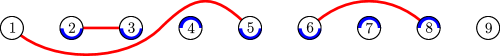
Remark 8.7.
Noncrossing arc diagrams and other similar objects have been used to model the bricks over hereditary and preprojective algebras of type A. In particular, (-sortable) arcs are in bijection with bricks, and (-sortable) noncrossing arc diagrams are in bijection with semibricks. One can then use noncrossing arc diagrams to compute information about morphisms and extensions between bricks, and thus also to model 2-term simple-minded collections. See, e.g., [BCZ19, BH22, Eno21, GIMO19, Hanb, HY23, Miz22] and references therein.
Cambrian lattices are semidistributive, so we can consider the canonical join complex and the canonical meet complex of (and we know these simplicial complexes are isomorphic by [Bar19, Corollary 5]). An element is join-irreducible if and only if it has exactly one descent, and this occurs if and only if contains a single arc. Therefore, establishes a one-to-one correspondence between the join-irreducible elements of and the -sortable arcs. Then for each , the noncrossing arc diagram corresponds to the canonical join representation of . It follows that the simplicial complex is isomorphic to the canonical join complex of . Say a noncrossing arc diagram in is maximal if it is a facet of . In other words, a noncrossing arc diagram in is maximal if it is not properly contained in another noncrossing arc diagram in . Let denote the set of maximal noncrossing arc diagrams in .
The preceding discussion yields the identity
| (8.3) |
8.4. Motzkin paths
A Motzkin path is a lattice path in the plane that consists of up (i.e., ) steps, down (i.e., ) steps, and horizontal (i.e., ) steps, starts at the origin, never passes below the horizontal axis, and ends on the horizontal axis. Let , , and denote up, down, and horizontal steps, respectively. Given a word over the alphabet , let , , and denote the number of , the number of ’s, and the number of ’s in , respectively. We can think of a Moztkin path as a word over the alphabet such that and for every prefix of . For example, the word represents the Motzkin path in Figure 3.
A peak of a Motzkin path is a point where an up step in ends and a down step in begins; the height of this peak is the number . If we view as a word over , then a peak corresponds to a consecutive occurrence of , and the height of the peak is , where is the prefix of that ends with the up step involved in the peak. The two peaks of the Motzkin path in Figure 3 are the points and .
Let denote the set of Motzkin paths of length , and let be the subset of consisting of Motzkin paths that do not have any peaks of height . Let and . Let
If is a nonempty Motzkin path, then either for some , or for some . This translates into the functional equation
which we can solve to find that
If is a nonempty Motzkin path with no peaks of height , then either for some nonempty and some , or for some . This translates into the functional equation
We can solve this equation and use the above formula for to obtain
| (8.4) |
Using Equation 8.4, one can readily check that the expression on the right-hand side of Equation 8.1 is
Therefore, in order to prove Equation 8.1, it suffices (by Equation 8.3) to exhibit a bijection such that for every .
8.5. The bijection
Throughout the remainder of this section, let us fix a positive integer and write . The map is given by
As in Section 8.3, we consider noncrossing arc diagrams drawn on points that are arranged horizontally and identified with the numbers from left to right.
Lemma 8.8.
If and , then is the left endpoint of an arc in , or is the right endpoint of an arc in (or both).
Proof.
Suppose instead that is not a left endpoint of an arc in and that is not a right endpoint of an arc in . Let be the unique -sortable arc whose endpoints are and . Because , it is straightforward to check that is a noncrossing arc diagram in . This contradicts the maximality of . ∎
Suppose . Let be the word , where for , we define
| (8.5) |
Lemma 8.8 guarantees that is well defined (i.e., that no letter in can be both and ). See Figure 4 for an illustration.
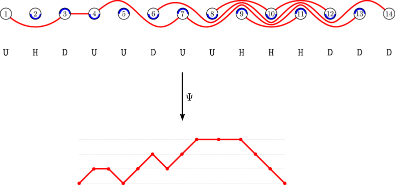
Proposition 8.9.
For each , we have and .
Proof.
Let , where the steps are as defined in Equation 8.5. It is immediate from Equation 8.5 that and are both equal to . In particular, .
Suppose is such that the prefix of satisfies . If , then is the number of elements of that are right endpoints of arcs in . Similarly, if , then is the number of elements of that are left endpoints of arcs in . It follows that either , or there is an arc from to in . In either case, it is immediate from Equation 8.5 that . Moreover, none of the arcs with left endpoints in have right endpoints in . If we had and , then we could add the arc from to to in order to form a larger noncrossing arc diagram in , contradicting the maximality of . Together, this shows that cannot pass below the horizontal axis and cannot have any peaks of height . Hence, . ∎
We can now state and prove the main theorem of this section; as mentioned at the end of Section 8.4, this theorem and Proposition 8.9 imply the identity in Equation 8.1, thereby settling the conjecture of Defant and Williams.
Theorem 8.10.
The map is a bijection.
Proof.
Given an arc and a vertical line that lies strictly between the endpoints of , let be the curve obtained from by deleting the portion of that lies to the right of . We call a curve obtained in this manner a partial arc.
Consider . Let us try to construct such that . We can build step by step from left to right. This process is illustrated in Figure 5. For the first step, we create a small partial arc that starts at the point . In general, at the -th step, we consider the point . At this point in time, there may be some partial arcs that were produced in the previous steps. If and , then we extend one of these partial arcs and attach it to the point in order to create an arc, and we extend the rest of the partial arcs above (if is odd) or below (if is even) the point . The condition that arcs cannot cross uniquely determines which partial arc we must attach to the point . During the same -th step, if and , then we create a new small partial arc that starts at the point .
To see that the above procedure succeeds in producing a noncrossing arc diagram in , we must check two things:
-
•
If and , then there is actually a partial arc from the first steps that we can attach to the point .
-
•
The total number of steps during which we create a new partial arc is equal to the total number of steps during which we attach a partial arc to a point to create an arc.
For the first item, note that the number of partial arcs remaining after the first steps is . Because is a Motzkin path, this quantity is nonnegative; furthermore, it can only be if the steps and are and (respectively) and form a peak of height . But has no peaks of height , so the number of partial arcs remaining after steps must actually be at least . The second bulleted item follows from the fact that .
Let us now show that the noncrossing arc diagram constructed through the above procedure is actually maximal in ; it will then follow immediately from the construction that . Note also that the steps outlined above for constructing were forced upon us; in other words, is injective.
Let denote the unique -sortable arc from to . Suppose by way of contradiction that there exist such that is not in and is a noncrossing arc diagram. We will assume is even; the case when is odd is almost identical. We consider three cases.
Case 1. Assume . Then we have and , so the steps and form a peak. Since does not cross any of the arcs in , none of the arcs in can pass below and above . Hence, every arc in whose left endpoint is in has its right endpoint in . It follows from the construction of that . But this implies that the peak formed by and has height , which contradicts the fact that has no peaks of height .
Case 2. Assume . Then the point is not the left endpoint of an arc in , and the point is not the right endpoint of an arc in . However, this implies that is both and , which is impossible.
Case 3. Assume . Note that . Since , there must be an arc in whose right endpoint is . The arc passes above and below . The left endpoint of cannot be since, if it were, the arcs and would cross. Therefore, passes above . The lower endpoint of also cannot be because is the left endpoint of . Therefore, passes below . However, this forces and to cross, which is a contradiction. ∎
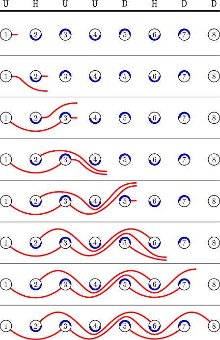
9. Maximum-Size Pop-Stack Orbits
Let be a finite irreducible Coxeter group. All Coxeter elements of are conjugate to each other, so they have the same group-theoretic order; this order is called the Coxeter number of and is denoted by . (It is also known that , where and are the number of reflection in and the number of simple reflections in , respectively.) Recall that, given a finite lattice , we write for the forward orbit of an element under the pop-stack operator. If is a Coxeter element of , then is a quotient of . Let be an arbitrary lattice quotient on . We begin this section by showing that is an upper bound for when is an arbitrary quotient of (Theorem 9.6). In the process, we also provide a formula for computing for any lattice quotient of the weak order. We then prove that this upper bound is tight when is a Cambrian lattice (Theorem 9.17). We also discuss how the techniques used in this section relate back to representation theory in Section 9.4.
9.1. Quotients of the weak order
As above, let be a finite lattice. An equivalence relation on is a lattice congruence provided that equivalence classes respect the meet and join operations in . That is, is a lattice congruence if for all satisfying , we have and .
Let be a lattice congruence. Let denote the equivalence class of an element under . One can define a lattice structure on the set of equivalence classes as follows. We set if and only if there exist and such that . We then have and . The lattice is called a lattice quotient of . Observe that there is a surjective lattice homomorphism that sends each element to its equivalence class . (See [Rea16, Proposition 9.5-4].)
Given an equivalence relation on , one can check that is a lattice congruence order-theoretically using the following result.
Proposition 9.1 ([Rea16, Proposition 9-5.2]).
An equivalence relation on a finite lattice is a lattice congruence if and only if the following three conditions hold:
-
•
Each equivalence class is an interval of .
-
•
The map that sends each element to the unique minimal element of its equivalence class is order-preserving.
-
•
The map that sends each element to the unique maximal element of its equivalence class is order-preserving.
Finally, we note that if is a lattice congruence on , then the map is a lattice homomorphism whose image (taken as an induced subposet of ) is isomorphic to the quotient . (Dually, the image of is also isomorphic to the quotient .)
Remark 9.2.
Although the subposet is a lattice in its own right, it meet and join operations may not coincide with those of . Said another way, is not generally a sublattice of . In general, the join operation of does coincide with that of ; dually, the meet operation of does coincide with that of . However, each -Cambrian lattice (of type ) is both a lattice quotient and sublattice of the weak order on .
Below, we realize an arbitrary lattice quotient of the weak order as the subposet induced by the image of , where is a lattice congruence. We have two main tasks as we consider the pop-stack operator on . First, we must we identify the lower covers of each ; this is done in the following lemma.
Lemma 9.3.
Let be a finite lattice, and let be a lattice congruence on . If , then the map restricts to a bijection from the set of elements covered by in to the set of elements covered by in .
Proof.
First assume that in , and let . Since is order-preserving, we have . Suppose that there exists with . We cannot have because is the largest element of lying below . Moreover, we cannot have because . Therefore, and are incomparable. This implies that (because and ). Since , we have . But this contradicts the fact that and are distinct elements of . From this contradiction, we deduce that in .
We have shown that restricts to a map from the set of elements covered by in to the set of elements covered by in ; we must show that it is bijective. To show it is injective, suppose instead that there exist distinct elements that are covered by in such that . Then , so , contradicting the fact that is the unique minimal element of . To prove surjectivity, suppose in . Then there exists such that . Since is order-preserving, we have . Thus, . ∎
Now that we have identified the lower covers of the elements of a lattice quotient , we describe the pop-stack operator on a lattice quotient of . It will be convenient to write and for the meet operation of and the meet operation of , respectively.
Proposition 9.4.
Let be a finite lattice, and let be a lattice congruence on . For , we have
Proof.
By Lemma 9.3, it suffices to show that for , we have . Observe that in . Since and are both in the image of , the desired result follows from the fact that is the largest element of lying below . ∎
Remark 9.5.
Let be a the weak order on a finite Coxeter group . Let be the -Cambrian congruence on . The fact that each -Cambrian lattice is a sublattice of the weak order implies that and the meet operation of the weak order commute (see, e.g., [Def22a, Lemma 3.1]). Hence,
We obtain equality from the first line to the second line because the meet taken in the -Cambrian lattice stays in the -Cambrian lattice (so the outermost acts as the identity). The equality from the second to the third line results from the fact that and the meet operation commute. Thus, we obtain the simpler expression for from Equation 6.3.
We now specialize to the case where is the weak order on and prove our main result of this subsection. Let denote a lattice quotient of coming from a congruence .
Theorem 9.6.
If is a lattice quotient of , then
Proof.
We may assume that is the subposet of , where is a lattice congruence on . We write and to denote meets and cover relations, respectively, in (while and will denote meets and cover relations in ). Define a map by
Note that
(recall that denotes the forward orbit of under ).
Following [Def22b], we say a map is compulsive if for all . [Def22b, Theorem 1.5] states that if is compulsive, then
Hence, it suffices to show that is compulsive.
Consider . By Lemma 9.3, we have
But then since for all , we have
On the other hand, whenever or . This shows that is compulsive. ∎
Remark 9.7.
One cannot weaken the hypothesis in Theorem 9.6 by assuming that is just a meet-semilattice quotient or a join-semilattice quotient. For example, suppose . Let be the meet-semilattice congruence on with one nontrivial equivalence class consisting of , , and . The lattice is a -element chain, so .
9.2. Heaps and combinatorial AR quivers
Our goal is now to show that the upper bound in Theorem 9.6 is tight when is a Cambrian lattice . We will do this by constructing an explicit element whose forward orbit under has size exactly . Our construction makes use of the combinatorial AR quivers of [STW, Section 9]. As we explain in Section 9.4, these are intimately related with the representation theory of the tensor algebra .
It will be convenient to think of the letters in a word over the alphabet as being distinct entities even if they represent the same simple reflection. For example, the two occurrences of in the word are considered to be different. If and are letters representing simple reflections and , then we let (recall that is the order of ). We can apply a commutation move to a word by swapping two consecutive letters and if (this move is not allowed if ). The commutation class of a word over is the set of words that can be obtained from via a sequence of commutation moves. We write if and are in the same commutation class.
Let be a word over . The heap of is the poset whose elements are the letters in (which we view as distinct from one another) and whose order relation is defined so that if and are two letters (which could represent the same simple reflection), then if and only if appears to the left of in every word in the commutation class of . A word is in the same commutation class as if and only if . More generally, is an order ideal of if and only if there exists a word such that .
Suppose is the heap of a word . We write for the element of represented by and write for the set of simple reflections that appear in . If , then and represent the same element of ; therefore, and depend only on (and not the particular word ). Let denote the set of order ideals of .
Let be a reduced word for a Coxeter element , and let denote the word obtained by concatenating with itself times. Let , and let denote the -th letter in that represents . For example, if , then
Lemma 9.8.
For each , the poset is ranked.
Proof.
Because is a tree, it is straightforward to see that is ranked. Let be the unique rank function of whose minimum value is . Let us extend this rank function to a map by letting . We claim that this map is a rank function on . To see this, suppose is a cover relation in . Then is an edge in . If appears before in , then we have and . If appears after in , then we have and . In either case, we compute that . ∎
Let be the rank function on that was constructed in the proof of Lemma 9.8. When we consider a heap that can be naturally identified with a convex subset of , the rank of an element of will simply be , the rank of in . We will also find it convenient to write
There is an involution given by ; this map is an automorphism of . We can extend to the set of words over by letting .
Let and ; note that and depend only on the Coxeter element (and not the reduced word ). It follows from [STW, Lemma 2.6.5] that
| (9.1) |
Therefore, we can think of as an order ideal of whose complement (in ) is . Define
Remark 9.9.
We have defined using Coxeter–Catalan combinatorics because we deemed this approach to be the most amenable for proving that . However, there is also a more direct lattice-theoretic way to define . The spine of , denoted , is the union of the maximum-length chains of . Thomas and Williams [TW19b] proved that is a distributive sublattice of . It is also known [TW19b] that
One can show that (where is the identity element).
Example 9.10.
Suppose . The edges in are for . The Coxeter number of is . The map is given by . Let and . The acyclic orientation of corresponding to is
Figure 6 shows the Hasse diagram of ; it is drawn sideways so that each cover relation is drawn with to the left of . As explained in Section 9.4, this Hasse diagram is referred to as the combinatorial AR quiver of in [STW, Section 9.2]. Note that is drawn by lining up copies of (depicted in different colors) in a row and adding (black) edges as appropriate. The columns are labeled from to from left to right; the column labeled consists of the elements of rank . The region shaded in yellow is , while the unshaded region is . The region outlined in blue is . Thus,
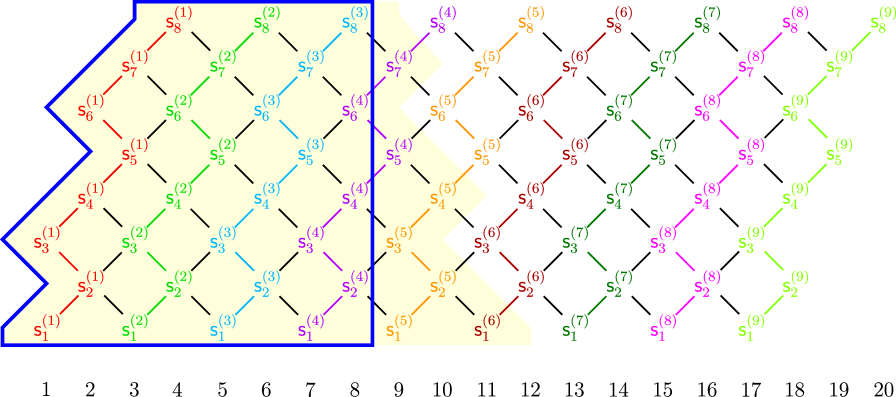
9.3. Realization of the upper bound
We need a little more preparation before we can prove that .
For , let
Note that for each , the parity of only depends on (and not ). Let
Then is a bipartition of the tree .
Lemma 9.11.
We have .
Proof.
We already know that , so we just need to prove the reverse containment. We will show that each element of has rank at least ; this will imply that the elements of with rank must belong to .
Fix a simple reflection , and let . Let be the smallest integer such that . Let be the smallest integer such that . Then is the number of letters in that represent , so it is also the number of letters in that represent . But the number of letters in that represent is , so . Hence,
Because is an automorphism of , the map is a poset isomorphism. It follows that . By definition, we have and , so
Rearranging this equation yields . Consequently,
In particular, . This shows that every element of that represents has rank at least . As was arbitrary, it follows that all of the elements of have rank at least .
Suppose , and let be the unique integer such that . It follows from the preceding paragraph that , so . This shows that . Hence, . ∎
Example 9.12.
Let us use Figure 6 to illustrate the proof of Lemma 9.11. Recall that, in this example, the map is given by . Let so that . Then , , , and . Note that and . We have , as Lemma 9.11 claims.
Let and , and fix reduced words and for and , respectively. The element is called a bipartite Coxeter element of . (In type A, this definition of coincides with that of either or from Section 8.1.) Let . Let be the word that begins with and alternates between and , using copies of and copies of . In other words,
It is known [Bou02, V.6 Exercise 2] that . Hence, for , the word is a reduced word for an element , and .
Lemma 9.13.
For each , we have .
Proof.
The reduced word ends with , and . Since all of the simple reflections in commute with each other, we have .
Now suppose by way of contradiction that . Let , and note that . Since , we have . Let
Then . We have
which is a contradiction because
Example 9.14.
Let . Our convention is that and that the edges of (each of which is unlabeled) are , , , . The Coxeter number of is . The map is given by , , and for all . Let and . The acyclic orientation of corresponding to is
We have and . The region outlined in blue in Figure 7 is (drawn sideways, similarly to Figure 6). The region shaded in yellow is . We have added the extra elements (and appropriate edges) to the left of in order to realize as the region enclosed by the black rectangle. The yellow shaded region that lies inside of the black rectangle is ; this illustrates how we can naturally identify with a subposet of .
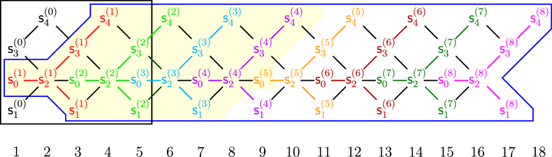
Lemma 9.15.
For each , we have .
Proof.
We have , so all of the elements of commute with each other. Therefore, . Because is an order ideal of whose complement (in ) is , we have , so . Now choose some ; we will show that .
Because for every , we can identify with a subposet of (as illustrated in Figure 7). We will also continue to use Equation 9.1 to view as an order ideal of whose complement is . We claim that is an upper set of . To see this, suppose and are such that in . Let be a simple reflection in such that . There is a unique integer such that . Then is maximal in . Since and are comparable (because ), we must have . It follows from Lemma 9.11 that ; in particular, . Because is an order ideal of , it contains . But , so . This proves that is an upper set of . Because is a reduced word for , it follows that (in the weak order). Consequently, .
Let be the unique element of rank in that represents . Because , there must be an element that represents . Because , we have in . But is an upper set of , so . As has rank , it must be in . This proves that , as desired. ∎
Lemma 9.16.
Let be a Coxeter element of . We have
Proof.
As before, let (resp. ) be the set of simple reflections such that the letters representing in have odd (resp. even) rank. For , let . In particular, , and . Suppose . We know that , so all of the elements of commute with each other. Along with Lemma 9.15, this implies that
We have , so it follows from Equation 6.1 that
Because is an order ideal of , we know by Remark 9.9 that is in the spine of ; in particular, it is in . Invoking Equation 6.3, we find that
As this is true for all , we deduce that
Combining Theorem 9.6 with Lemma 9.16 yields our last main result.
Theorem 9.17.
Let be a finite irreducible Coxeter group, and let be a Coxeter element. The maximum size of a forward orbit under is exactly the Coxeter number of .
9.4. Heaps and representation theory
We conclude this section with a brief explanation of how the heap of a -sortable word relates to representation theory of .
Let be an arbitrary finite-dimensional algebra. A morphism in is said to be irreducible if it is not an isomorphism and whenever , , and are such that , we have that either or is an isomorphism. For , we denote by the linear subspace of spanned by the irreducible morphisms. The Auslander–Reiten (AR) quiver of is then the directed graph defined as follows.
-
•
The vertices of the AR quiver are the indecomposable objects in .
-
•
For any two vertices , the number of arrows in the AR quiver coincides with the dimension of .
Now let be a word over . In [STW, Section 9.2], the Hasse diagram of is referred to as the combinatorial AR quiver of . To explain this, consider the special case when . By [STW, Theorem 9.3.1], there is a bijection . Under this bijection, we have if and only if there is an irreducible morphism from to . Thus, under the bijection , the Hasse diagram of is precisely the AR quiver of . (In this setting, the dimension of does not exceed 1.) In particular, the drawing of shown as the shaded yellow part of Figure 6 agrees with the standard way of embedding the AR quiver of in the plane; see, e.g., [Sch14, Section 3.1].
It is also shown in [STW, Theorem 9.3.1] that, for all , the projective module satisfies . Because every nonzero morphism can be written as a composition of irreducible morphisms, the first copy of in thus provides a visualization of the well-known fact that .
10. Future Directions
10.1. Images
Consider the linear Coxeter element of . The Cambrian lattice is the -st Tamari lattice. Hong [Hon22] proved that the size of the image of is the -th Motzkin number (i.e., the number of Motzkin paths of length ). In Section 8, we determined the size of the image of , where is a bipartite Coxeter element of . Using these formulas, one can verify that . Numerical evidence has led us to conjecture that the linear and bipartite Coxeter elements are, in some sense, extremal with regard to the sizes of the images of pop-stack operators.
Conjecture 10.1.
For every Coxeter element of , we have
10.2. Forward orbits
Suppose is a finite lattice, and let . Let
be the set of elements of whose forward orbits under attain the maximum possible size.
Let be a Coxeter element of a finite irreducible Coxeter group . We saw in Theorem 9.17 that is the Coxeter number , and we constructed an explicit element . However, we said nothing about the other elements . In the case when and is the linear Coxeter element (i.e., is the -st Tamari lattice), it is known that is the -st Catalan number [Def22a]. It would be interesting to understand for other choices of . In particular, we have the following conjecture.
Conjecture 10.2.
Assume , and let be the bipartite Coxeter element of type given by
The set of elements of whose forward orbits under the pop-stack operator have size is given by
The original use of the term pop-stack comes from the setting where is the weak order on ; in this case, Ungar proved that is (which is the Coxeter number of ).
Question 10.3.
What can be said about ?
Defant [Def22b] proved that if is a finite irreducible Coxeter group with Coxeter number , then . In Theorem 9.6, we found that whenever is a lattice quotient of , and we saw in Theorem 9.17 that this inequality is an equality whenever is a Cambrian lattice. We are naturally led to ask the following questions.
Question 10.4.
Let be a finite irreducible Coxeter group with Coxeter number . For which lattice quotients of is it the case that ?
Question 10.5.
Let be a lattice quotient of a finite lattice . Is it necessarily the case that
10.3. Generalizations
It would be interesting to see how much of our work on Cambrian lattices can be extended to more general families of lattices. For example, it could be interesting to study the pop-stack operators on -Cambrian lattices, which were introduced by Stump, Thomas, and Williams [STW].
Appendix A Proof of Theorem 4.6
In this appendix, we prove Theorem 4.6. More precisely, we prove only the first half of the theorem, as the second half is just the dual. We follow arguments similar to those appearing in [HI21a, Section 3] and [KY14, Section 7.2]. The main difference is that we work almost exclusively in the category (with the exception of a portion of the proof of Lemma A.1 below), while the referenced papers work primarily in the bounded derived category.
In the arguments that follow, we recall that for any wide subcategory and any , we have and . On the other hand, we may have that for .
Lemma A.1.
Let be SM compatible. Let , , and .
-
(1)
The map induced by the short exact sequence from Equation 4.1 is bijective.
-
(2)
The map induced by the short exact sequence from Equation 4.1 is injective.
Proof.
1 Since is a wide subcategory, we have that . We have since is a wide subcategory. Now, is a Serre subcategory of , so in particular, there is a torsion pair in . This implies that . From the exact sequence
we therefore conclude that the induced map is a bijection.
2 We first claim that . We know from Theorem 3.7 that there exists such that is a 2-term simple-minded collection. Then, as in [KY14, Lemma 7.8], there exist a finite-dimensional algebra and a triangle functor
such that the following hold:
-
•
.
-
•
acts as the identity on .
-
•
For all , the induced map is a bijection, and the induced map is an injection.
Now, is a Serre subcategory of and a wide subcategory of . Thus, taking and above, we find that induces an inclusion . To prove the claim, it therefore suffices to show that .
Consider the following commutative diagram, where the first row consists of projective covers and syzygies in and the second row consists of projective covers and syzygies in .
Since is a Serre subcategory of , every module in has the same top in both and in . Thus, the induced map , and so also , must be surjective. Now for , we get an induced exact sequence
where the last term is 0 because is projective in . Since and have the same top, this implies that , and hence also that . Moreover, we see that the top of is a direct summand of the top of , and thus that the induced map is surjective. From the snake lemma, this means there is a surjective map . On the other hand, since is a Serre subcategory of . It follows that is surjective. In particular, the induced map is injective. This proves the claim.
Now consider the following commutative diagram of projective covers and syzygies in :
The induced map is a (split) epimorphism. Consequently, we have a surjection . On the other hand, we have that , as observed in the proof of 1. Similarly, we have since is a Serre subcategory of . We conclude that . In particular, the induced map
is injective. Together with the claim, the fact that then implies the result. ∎
Lemma A.2.
Let be SM compatible. Let , , and .
-
(1)
The map induced by is bijective.
-
(2)
The map induced by is injective.
Proof.
1 Let be such that . Equivalently, we have . Note that since is a wide subcategory. Since is a right minimal -approximation, it follows that ; i.e., . This shows that the induced map is injective; the fact that it is surjective comes from the definition of an approximation.
Proposition A.3 (Theorem 4.6, 1).
Let be SM compatible, and let . Then is a semibrick pair.
Proof.
The proof is similar to that of [HI21a, Proposition 3.5]. For readability, let and .
Claim 1: The set is a semibrick.
Let . First suppose that . If , then there is nothing to show since is a semibrick. If for some such that is surjective, then because and .
Now suppose that there exists such that is surjective and We first consider the case . Then we have a long exact sequence
where we know the indicated maps are 0 by Lemma A.2.
It remains to consider the case where there exists such that is surjective and . We then have a long exact sequence
where the last term is 0 by the case considered above. Similarly, we have a long exact sequence
Together, these sequences show that . In particular, setting , we conclude that is a brick. This proves the claim.
Claim 2: We have for all and .
Again, there are two possibilities. Suppose first that there exists such that . Then we have a long exact sequence
where we know the indicated maps are 0 by Lemma A.1. This proves the claim in this case.
The other case to consider is that in which there exists such that is injective and . In this case, we have a long exact sequence
where again we know the indicated maps are 0 by Lemma A.2. This proves the claim.
Claim 3: We have for all and such that is surjective.
Again, there are two possibilities. Suppose first that there exists such that . Then because . Moreover, we have a long exact sequence
where the first term is 0 by Claim 2 and the last term is 0 because . This proves the claim in this case.
The other case to consider is that in which there exists such that is injective and . The fact that then follows from the fact that . Moreover, we have an exact sequence
where the first and last terms are 0 by Claim 2. Likewise, we have an exact sequence
where the first and last terms are 0 since . Together, these two exact sequences yield that , as desired.
Claim 4: The set is a semibrick.
Let . First suppose that there exist such that and . Then there is an exact sequence
where the first and last terms are 0 by Claim 2. We also have a long exact sequence
Together, these sequences show that . In particular, by setting , we conclude that is a brick. This proves the claim in this case.
Now suppose there exists such that is injective and and that there exists such that . Then since . We then have an exact sequence
where the first term is 0 by Claim 2. Similarly, we have an exact sequence
where the first term is 0 by Claim 2 and the last term is 0 because . We conclude that .
It remains to consider the case where there exist such that and are injective, , and . As in earlier cases, we have an exact sequence
where the first and last terms are 0 by Claim 2. Similarly, we have an exact sequence
where the first and last terms are 0 since . We again conclude that . This concludes the proof. ∎
Proposition A.4 (Theorem 4.6,2–5).
Let be SM compatible, and let . Write .
-
(1)
If is an SM compatible semibrick pair such that and , then we have and .
-
(2)
if and only if .
-
(3)
is completable if and only if is completable.
-
(4)
If , then .
Proof.
1 First note that and therefore that by construction.
Now let so that . Then Lemma A.1 tells us that the map is a minimal right -approximation of that is injective and has cokernel . It follows that .
It remains to consider . Suppose first that is injective. For any , the quotient map induces a bijection . Thus, is a minimal right -approximation of that is surjective and has kernel . We conclude that .
It remains to consider the case when is surjective. Let . We consider the commutative diagram
where the bottom row consists of the injective envelope and first cosyzygy of in . The vertical maps are induced by the fact that the top row is an element of , so in particular, the right square is a pullback. Now for , we have an exact sequence
where the first and last terms are 0 since . Moreover, we have a canonical isomorphism since is a wide subcategory of . We conclude that induces a bijection , so it is a minimal right -approximation. Thus, the top row of our diagram coincides with the short exact sequence described above Definition 4.4. We conclude that .
2 Let . Then the short exact sequence corresponds to a triangle
in . Thus, any triangulated subcategory that is closed under direct summands and contains (some shift of) will contain if and only if it contains . Similarly, for , we have a triangle
where either or . Thus again, any triangulated subcategory that is closed under direct summands and contains will contain if and only if it contains . This proves the result.
4 Recall that and by Theorem 3.7.
The fact that follows from the definitions. Hence, let . Then for all such that is injective, we necessarily have that . It therefore suffices to show that for such that is surjective, we have that if and only if . The inclusion holds in general, so suppose that . Then the fact that implies that as well. This concludes the proof. ∎
Acknowledgments
Colin Defant was supported by the National Science Foundation under Award No. 2201907 and by a Benjamin Peirce Fellowship at Harvard University. Eric Hanson was partially supported by Canada Research Chairs CRC-2021-00120 and by NSERC Discovery Grants RGPIN-2022-03960 and RGPIN/04465-2019. A portion of this work was completed while Eric Hanson was a postdoctoral fellow at l’Université du Québec à Montréal and l’Université de Sherbrooke. We are grateful to Nathan Williams for helpful conversations.
References
- [AM17] A. Aihara and Y. Mizuno, Classifying tilting complexes over preprojective algebras of Dynkin type, Algebra Number Theory 11 (2017), no. 6, 1287–1315.
- [AN09] S. Al-Nofayee, Simple objects in the heart of a -structure, J. Pure Appl. Algebra 213 (2009), no. 1, 54–59.
- [AHI+] T. Aoki, A. Higashitani, O. Iyama, R. Kase, and Y. Mizuno, Fans and polytopes in tilting theory I: Foundations, arXiv:2203.15213.
- [Asa20] S. Asai, Semibricks, Int. Math. Res. Not. IMRN 2020 (2020), no. 16, 4993–5054.
- [AP22] S. Asai and C. Pfeifer, Wide subcategories and lattices of torsion classes, Algebr. Represent. Theory 25 (2022), 1611–1629.
- [ABB+19] A. Asinowski, C. Banderier, S. Biley, B. Hackl, and S. Linusson, Pop-stack sorting and its image: permutations with overlapping runs, Acta Math. Univ. Comenianae 88 (2019), 395–402.
- [ASS06] I. Assem, D. Simson, and A. Skowroński, Elements of the representation theory of associative algebras, volume 1: techniques of representation theory, London Math. Soc. Stud. Texts, vol. 65, Cambridge University Press, Cambridge, 2006.
- [ARS95] M. Auslander, I. Reiten, and S. O. Smalø, Representation theory of Artin algebras, Cambridge Stud. Adv. Math., vol. 36, Cambridge University Press, Cambridge, 1995.
- [Bar19] E. Barnard, The canonical join complex, Electron. J. Combin. 26 (2019).
- [BCZ19] E. Barnard, A. Carroll, and S. Zhu, Minimal inclusions of torsion classes, Algebr. Comb. 2 (2019), no. 5, 879–901.
- [BH] E. Barnard and E. J. Hanson, Exceptional sequences in semidistributive lattices and the poset topology of wide subcategories, arXiv:2209.11734.
- [BH22] E. Barnard and E. J. Hanson, Pairwise compatibility for 2-simple minded collections II: preprojective algebras and full rank semibirck pairs, Ann. Comb. 26 (2022), 803–855.
- [BR18] E. Barnard and N. Reading, Coxeter-biCatalan combinatorics, J. Algebraic Combin. 47 (2018), no. 2, 241–300.
- [BTZ21] E. Barnard, G. Todorov, and S. Zhu, Dynamical combinatorics and torsion classes, J. Pure Appl. Algebra 225 (2021).
- [BB05] A. Björner and F. Brenti, Combinatorics of coxeter groups, Graduate Texts in Mathematics, vol. 231, Springer, Berlin, Heidelberg, 2005.
- [Bou02] N. Bourbaki, Lie groups and Lie algebras Chapters 4-6, Springer–Verlag, Berlin, Copyright Information Springer-Verlag Berlin, Heidelberg, 2002.
- [BY13] T. Brüstle and D. Yang, Oriented exchange graphs, In (D. J. Benson, H. Krause, and A. Skowroński, eds.) Advances in Representation Theory of Algebras, EMS Series of Congress Reports, vol. 9, 2013.
- [CS] Y. Choi and N. Sun, The image of the pop operator on various lattices, To appear in Adv. Appl. Math.
- [CG19] A. Claesson and B. Á. Guðmundsson, Enumerating permutations sortable by passes through a pop-stack, Adv. Appl. Math. 108 (2019), 79–96.
- [CGP21] A. Claesson, B. Á Guðmundsson, and J. Pantone, Counting pop-stacked permutations in polynomial time, Experiment. Math. (2021).
- [Def22a] C. Defant, Meeting covered elements in -tamari lattices, Adv. Appl. Math. 134 (2022).
- [Def22b] C. Defant, Pop-stack-sorting for Coxeter groups, Comb. Theory 2 (2022).
- [DKW] C. Defant, N. Kravitz, and N. Williams, The Ungar games, arXiv:2302.06552.
- [DL] C. Defant and R. Li, Ungarian Markov chains, arXiv:2301.08206.
- [DW23] C. Defant and N. Williams, Semidistrim lattices, Forum Math. Sigma 11 (2023), no. 50, 1–35.
- [DIJ17] L. Demonet, O. Iyama, and G. Jasso, -tilting finite algebras, bricks, and -vectors, Int. Math. Res. Not. IMRN 2019 (2017), no. 3, 852–892.
- [DIR+23] L. Demonet, O. Iyama, N. Reading, I. Reiten, and H. Thomas, Lattice theory of torsion classes: beyond -tilting theory, Trans. Amer. Math. Soc. Ser. B 10 (2023), 542–612.
- [Dic66] S. E. Dickson, A torsion theory for abelian categories, Trans. Amer. Math. Soc. 121 (1966), no. 1, 223–235.
- [DR75] V. Dlab and C. M. Ringel, On algebras of finite representation type, J. Algebra 33 (1975), 306–394.
- [DR76] V. Dlab and C. M. Ringel, Indecomposable representations of graphs and algebras, Mem. Am. Math. Soc. 6 (1976).
- [Eno21] H. Enomoto, Bruhat inversions in Weyl groups and torsion-free classes over preprojective algebras, Comm. Algebra 49 (2021), no. 5, 2156–2189.
- [Eno22] H. Enomoto, Rigid modules and ICE-closed subcategories in quiver representations, J. Algebra 594 (2022), 364–388.
- [Eno23] H. Enomoto, From the lattice of torsion classes to the posets of wide subcategories and ICE-closed subcategories, Algebr. Represent. Theory (2023).
- [ES22] H. Enomoto and A. Sakai, ICE-closed subcategories and wide -tilting modules, Math. Z. 300 (2022), 541–577.
- [FJN95] R. Freese, J. Jezek, and J. Nation, Free lattices, Mathematical Surveys and Monographs, vol. 42, American Mathematical Society, 1995.
- [GIMO19] A. Garver, K. Igusa, J. P. Matherne, and J. Ostroff, Combinatorics of exceptional sequences in type A, Electron. J. Combin. 26 (2019), no. 1.
- [GM19] A. Garver and T. McConville, Lattice properties of oriented exchange graphs and torsion classes, Algebr. Represent. Theory 22 (2019), 43–78.
- [GL91] W. Geigle and H. Lenzing, Perpendicular categories with applications to representations and sheaves, J. Algebra 144 (1991), no. 2, 273–343.
- [Hana] E. J. Hanson, A facial order for torsion classes, arXiv:2305.06031.
- [Hanb] E. J. Hanson, -exceptional sequences and the shard intersection order in type A, arXiv:2303.11517.
- [HI21a] E. J. Hanson and K. Igusa, Pairwise compatibility for 2-simple minded collections, J. Pure Appl. Algebra 225 (2021), no. 6.
- [HI21b] E. J. Hanson and K. Igusa, -cluster morphism categories and picture groups, Comm. Alg. 49 (2021), no. 10, 4376–4415.
- [HW] W. Hara and M. Wemyss, Spherical objects in dimension two and three, arXiv:2206.11552.
- [HY23] E. J. Hanson and X. You, Morphisms and extensions between bricks over preprojective algebras of type A, J. Algebra (2023).
- [Hon22] L. Hong, The pop-stack-sorting operator on Tamari lattices, Adv. Appl. Math. 139 (2022).
- [ITW] K. Igusa, G. Todorov, and J. Weyman, Picture groups of finite type and cohomology in type , arXiv:1609.02636.
- [IT09] C. Ingalls and H. Thomas, Noncrossing partitions and representations of quivers, Compos. Math. 145 (2009), no. 6, 1533–1562.
- [IRRT18] O. Iyama, N. Reading, I. Reiten, and H. Thomas, Lattice structure of Weyl groups via representation theory of preprojective algebras, Compos. Math. 154 (2018), no. 6, 1269–1305.
- [IRTT15] O. Iyama, I. Reiten, H. Thomas, and G. Todorov, Lattice structure of torsion classes for path algebras, Bull. Lond. Math. Soc. 47 (2015), no. 4, 639–650.
- [Jas15] G. Jasso, Reduction of -tilting modules and torsion pairs, Int. Math. Res. Not. IMRN 2015 (2015), no. 16, 7190–7237.
- [KQ15] A. King and Y. Qiu, Exchange graphs and Ext quivers, Adv. Math. 285 (2015), 1106–1154.
- [KY14] S. Koenig and D. Yang, Silting objects, simple-minded collections, -structures and co--structures for finite-dimensional algebras, Doc. Math. 19 (2014), 403–438.
- [KS] M. Kontsevich and Y. Soibelman, Stability structures, motivic Donaldson-Thomas invariants and cluster transformations, arXiv:0811.2435.
- [Kül17] J. Külshammer, Pro-species of algebras I: Basic properties, Algebr. Represent. Theory 20 (2017), no. 5, 1215–1238.
- [LW] Y. Luo and J. Wei, Boolean lattices of torsion classes over finite-dimensional algebras, arXiv:2303.15802.
- [MŠ17] F. Marks and J. Šťovíček, Torsion classes, wide subcategories, and localisations, Bull. Lond. Math. Soc. 49 (2017), no. 3.
- [Miz14] Y. Mizuno, Classifying -tilting modules over preprojective algebras of Dynkin type, Math. Z. 277 (2014), no. 3-4, 665–690.
- [Miz22] Y. Mizuno, Arc diagrams and 2-term simple-minded collections of preprojective algebras of type A, J. Algebra 595 (2022), 444–478.
- [MT20] Y. Mizuno and H. Thomas, Torsion pairs for quivers and the Weyl groups, Selecta Math. 3 (2020), no. 46.
- [Müh19] H. Mühle, The core label order of a congruence-uniform lattice, Algebra Universalis 80 (2019).
- [PS19] L. Pudwell and R. Smith, Two-stack-sorting with pop stacks, Australas. J. Combin. 74 (2019), 179–195.
- [Rea04] N. Reading, Lattice congruences of the weak order, Order 21 (2004), 315–344.
- [Rea06] N. Reading, Cambrian lattices, Adv. Math. 205 (2006), 313–353.
- [Rea07] N. Reading, Clusters, Coxeter-sortable elements and noncrossing partitions, Trans. Amer. Math. Soc. 359 (2007), no. 12, 5931–5958.
- [Rea11] N. Reading, Noncrossing partitions and the shard intersection order, J. Algebraic Combin. 33 (2011), 483–530.
- [Rea15] N. Reading, Noncrossing arc diagrams and canonical join representations, SIAM J. Discrete Math. 29 (2015).
- [Rea16] N. Reading, Lattice theory of poset of regions, In (G. Grätzer and F. Wehrung, eds.) Lattice Theory: Special Topics and Applications, vol. 2, Birkhäuser, 2016.
- [RS11] N. Reading and D. E Speyer, Sortable elements in infinite Coxeter groups, Trans. Amer. Math. Soc. 363 (2011), no. 2, 699–761.
- [RST21] N. Reading, D. E Speyer, and H. Thomas, The fundamental theorem of finite semidistributive lattices, Selecta Math. 27 (2021), no. 59.
- [Ric02] J. Rickard, Equivalences of derived categories for symmetric algebras, J. Algebra 257 (2002), 460–481.
- [Rin76] C. M. Ringel, Representations of -species and bimodules, J. Algebra 41 (1976), 269–302.
- [The23] The Sage Developers, Sagemath, the Sage Mathematics Software System (Version 9.2), 2023, https://www.sagemath.org.
- [Sak] A. Sakai, Classifying -structures via ICE-closed subcategories and a lattice of torsion classes, arXiv:2307.11347.
- [Sch14] R. Schiffler, Quiver representations, CMS Books in Mathematics/Ouvrages de Mathématiques de la SMC, Springer, Cham, 2014.
- [STW] C. Stump, H. Thomas, and N. Williams, Cataland: Why the Fuß, To appear in Mem. Amer. Math. Soc.
- [Tho06] H. Thomas, An analogue of distributivity for ungraded lattices, Order 23 (2006), 249–269.
- [Tho21] H. Thomas, An introduction to the lattice of torsion classes, Bull. Iranian Math. Soc. (2021).
- [TW19a] H. Thomas and N. Williams, Independence posets, J. Comb. 10 (2019), no. 3, 545–578.
- [TW19b] H. Thomas and N. Williams, Rowmotion in slow motion, Proc. Lon. Math. Soc. 119 (2019), no. 5, 1149–1178.
- [Ung82] P. Ungar, noncollinear points determine at least directions, J. Combin. Theory Ser. A 33 (1982), 343–347.