[Appendix]tocatoc \AfterTOCHead[toc] \AfterTOCHead[atoc]
Position: Adopt Constraints Over Penalties
in Deep Learning
Abstract
Recent efforts to develop trustworthy AI systems with accountability guarantees have led to widespread use of machine learning formulations incorporating external requirements, or constraints. These requirements are often enforced via penalization—adding fixed-weight terms to the task loss. We argue this approach is fundamentally ill-suited since there may be no penalty coefficient that simultaneously ensures constraint satisfaction and optimal constrained performance, i.e., that truly solves the constrained problem. Moreover, tuning these coefficients requires costly trial-and-error, incurring significant time and computational overhead. We, therefore, advocate for broader adoption of tailored constrained optimization methods—such as the Lagrangian approach, which jointly optimizes the penalization “coefficients” (the Lagrange multipliers) and the model parameters. Such methods \raisebox{-.7pt}{{\hspace{-0.8mm} \small1}}⃝ truly solve the constrained problem and do so accountably, by clearly defining feasibility and verifying when it is achieved, \raisebox{-.7pt}{{\hspace{-0.8mm} \small2}}⃝ eliminate the need for extensive penalty tuning, and \raisebox{-.7pt}{{\hspace{-0.8mm} \small3}}⃝ integrate seamlessly with modern deep learning pipelines.
1 Introduction
The rapidly advancing capabilities of AI systems—exemplified by recent models like GPT-4 (OpenAI, 2023) and Gemini (Gemini Team, 2024)—have enabled their deployment across a wide range of domains, including sensitive applications such as credit risk assessment (Bhatore et al., 2020), recidivism prediction (Larson et al., 2016), and autonomous driving (Bachute and Subhedar, 2021). These developments have raised concerns regarding the reliability, interpretability, fairness, and safety of such tools (Dilhac et al., 2018), prompting increasing calls for their regulation and standardization (European Parliament, 2024).
In response, ensuring that models satisfy desirable or mandated properties has become a central goal in deep learning. A principled approach is to express these requirements as constraints, embedding them into the optimization process to guide training toward compliant models. This procedure ensures accountability: compliance is demonstrated by verifying whether the constraints are satisfied. Such constrained learning problems have been applied in fairness (Cotter et al., 2019b) and safety (Dai et al., 2024), among others.
To solve these problems, the deep learning community has predominantly adopted the penalized approach (Chen et al., 2016; Kumar et al., 2018; Louizos et al., 2018; Higgins et al., 2017; Zhu et al., 2017; Brouillard et al., 2020; Chakraborty et al., 2025; Shi et al., 2025; Dunion et al., 2023), which incorporates constraints into the objective via fixed-coefficient penalty terms and minimizes the resulting function (see §2.1 or (Ehrgott, 2005, §3)). This approach is applicable when all functions are differentiable and integrates naturally with standard tools for unconstrained deep learning optimization, such as Adam (Kingma and Ba, 2015) and learning rate schedulers.
However, as detailed in §3, this approach has two major drawbacks: \raisebox{-.7pt}{{\hspace{-0.8mm} \small1}}⃝ it may fail when the constrained problem is non-convex—as is common in deep learning—since there may be no choice of penalty coefficients for which the penalized minimizer optimally solves the constrained problem; and \raisebox{-.7pt}{{\hspace{-0.8mm} \small2}}⃝ tuning coefficients to obtain a desirable solution is often challenging, typically requiring repeated trial-and-error model training runs that waste both computational resources and development time.
Instead, we advocate for a paradigm shift toward broader adoption of tailored constrained optimization methods in deep learning—approaches more likely to truly solve the constrained problem while reducing the burden of hyperparameter tuning. The position of this paper is summarized as follows:
Deep learning researchers and practitioners should avoid the penalized approach and instead consider tailored constrained optimization methods—whenever the problem has explicit targets for some functions, that is, when it naturally fits a constrained learning formulation.111Even in multi-objective settings where all functions are minimized, we argue constrained formulations may be preferable to penalized ones for their superior ability to explore optimal trade-offs. See §3.1 for details.
In §4.2, we contrast a bespoke constrained method—the Lagrangian approach (Arrow et al., 1958), which also reformulates constrained problems via a linear combination of the objective and constraints—with the penalized approach to illustrate the superiority of principled constrained methods over penalization. The key distinction is that the Lagrangian approach is adaptable, as it optimizes its coefficients—the multipliers—instead of fixing them in advance. This adaptability underpins its effectiveness and has led to its widespread adoption for (principled) constrained deep learning (Robey et al., 2021; Dai et al., 2024; Stooke et al., 2020; Hashemizadeh et al., 2024; Hounie et al., 2023b; Elenter et al., 2022; Gallego-Posada et al., 2022).
Moreover, constrained optimization algorithms integrate easily with deep learning frameworks such as PyTorch (Paszke et al., 2019) and TensorFlow (Abadi et al., 2016), via open-source libraries like Cooper (Gallego-Posada et al., 2025) and TFCO (Cotter et al., 2019c). This integration lessens friction that might otherwise lead practitioners to favor penalized approaches. Beyond this practicality, constrained methods offer benefits such as support for non-differentiable constraints (Cotter et al., 2019b) and scalability to problems with infinitely many constraints (Narasimhan et al., 2020) (see §4.3).
Finally, we highlight some limitations of current constrained deep learning algorithms in §5, aiming to encourage further research into methods better tailored to such large-scale and non-convex settings.
Alternative views. While we advocate in favor of constrained deep learning, it may not be ideal in applications where the goal is to optimize all objectives simultaneously or where acceptable constraint levels cannot be clearly defined. In such cases, bespoke methods may be more appropriate—though the constrained approach remains applicable (see Ehrgott (2005, §4.1) for multi-objective settings and Hounie et al. (2024) for cases where constraint levels are unknown or flexible).
Notably, in convex settings, the penalized and constrained formulations are equivalent (see §2.1), making the penalized approach appealing: it converts the problem into an unconstrained one and avoids the need for specialized constrained optimization techniques. However, we stress the limitations of penalty-based methods in constrained deep learning, where convexity is rare.
Scope. We primarily focus on inequality-constrained problems, as constrained deep learning setups that rely on penalization are typically framed via inequalities. For completeness, however, we present both the penalized (§2.1) and Lagrangian (§4.1) approaches for general constrained problems, including equality constraints. While the penalized approach is not commonly used for equality-constrained problems, we emphasize that it inherits the same drawbacks as in the inequality case—along with the added risk of failing to recover any feasible solution at all (see §3.1)—and should also be avoided.
Related works. Many of the ideas presented in this paper are not new. For example, the inability of penalization to fully explore all optimal trade-offs between non-convex functions is a well-established result (Ehrgott, 2005, Ex. 4.2), and has also been raised in the context of deep learning optimization (Degrave and Korshunova, 2021a; Gallego-Posada et al., 2022; Gallego-Posada, 2024). Likewise, the difficulty of tuning penalty coefficients is a common critique in constrained deep learning and is often cited as a key motivation for adopting the Lagrangian approach instead. Where prior works typically mention these issues only in passing, this position paper consolidates, formalizes, and expands on them, offering a comprehensive and standalone perspective. We especially acknowledge the blog posts by Degrave and Korshunova (2021a, b), which share similar goals; we complement them with greater rigor and a perspective grounded in constrained optimization expertise.
2 Background
Let , and be twice-differentiable functions over . We consider the constrained optimization problem:
| (1) |
where and specify the constraint levels, and denotes element-wise inequality. We refer to as the objective function, and to and as the inequality and equality constraints, respectively.
A point is feasible if it satisfies the constraints, and is a constrained minimizer if it is feasible and satisfies for all feasible . An inequality constraint is active at if it holds with equality, i.e. . Equality constraints are always active at feasible points.
Constrained formulations are ubiquitous in machine learning. Typically, the objective captures the learning task, while the constraints steer optimization toward models satisfying desirable properties such as sparsity (Gallego-Posada et al., 2022), fairness (Cotter et al., 2019b) or safety (Dai et al., 2024). For example, in a sparsity-constrained classification task, may represent the cross-entropy loss over model parameters , while a constraint such as enforces a bound on the number of nonzero parameters. In some settings, however, learning is directly embedded in the constraints, as in SVMs and Feasible Learning (Ramirez et al., 2025).
A key distinction between the constrained problem in Eq.˜1 and a corresponding multi-objective optimization problem—where , , and are all minimized—is that here and need only be satisfied, not optimized. In constrained optimization, only solutions that meet all constraints are admissible; any minimizer of that violates them is disregarded, regardless of its objective value.222In practice, small numerical violations of the constraints are often tolerated.
Optimality. In unconstrained differentiable optimization, stationarity of the objective is a necessary condition for optimality. In constrained problems, however, stationary points of can be infeasible, and optimal solutions may lie on the boundary of the feasible set () without being stationary points of the objective. To characterize optimality in constrained problems, we define the Lagrangian:
| (2) |
where and are the Lagrange multipliers associated with the inequality and equality constraints, respectively. We refer to as the primal variables, and to and as the dual variables.
A necessary condition for constrained optimality of is the existence of multipliers and such that is a stationary point of the Lagrangian333 For convenience, we overload the term “stationary point” to include not only points where the gradient vanishes but also all other candidate optima such as boundary points (where all non-boundary variables have zero gradients). This definition enables us to capture all candidate optima under a unified notion of stationarity. For the Lagrangian, this includes both classical stationary points and points where for some (or several) indices , provided the usual stationarity conditions hold with respect to , , and the remaining terms. —this is equivalent to satisfying the Karush-Kuhn-Tucker (KKT) first-order conditions (Boyd and Vandenberghe, 2004, §5.5.3). A sufficient condition is that is positive definite in all directions within the null space of the active constraints and that strict complementary slackness holds (see Bertsekas (2016, Prop. 4.3.2) for details). Under regularity conditions at a constrained minimizer —such as Mangasarian-Fromovitz (Mangasarian and Fromovitz, 1967)—the existence of corresponding multipliers and satisfying these conditions is guaranteed.
A saddle-point of —where minimizes and , maximize—yields a constrained minimizer of Eq.˜1. However, note that being a saddle-point is a stronger condition than satisfying the KKT conditions and is not necessary for optimality: in general, need not minimize to be constrained-optimal, and need not be positive definite in all directions. That is, the Lagrangian may be strictly concave in some (infeasible) directions—unlike in unconstrained minimization, where strict concavity at a point precludes its optimality.
This distinction is important because saddle-points of the Lagrangian may not exist for general non-convex problems, yet stationary points corresponding to solutions to Eq.˜1 can still exist under constraint qualifications (e.g., see Example˜1). Moreover, even when constraint qualifications fail, asymptotic KKT conditions still hold at constrained minimizers : for every , -approximate stationary points of exist—even if forming exact stationary points including may require or (Birgin and Mart´ınez, 2014, Thm. 3.1).
Constrained deep learning—where represents the parameters of a neural network and evaluating , , and involves computations over data—presents unique challenges: \raisebox{-.7pt}{{\hspace{-0.8mm} \small1}}⃝ it is large-scale, often involving billions of parameters; \raisebox{-.7pt}{{\hspace{-0.8mm} \small2}}⃝ non-convex, due to network nonlinearities; and \raisebox{-.7pt}{{\hspace{-0.8mm} \small3}}⃝ stochastic, as , , and are typically estimated from mini-batches. These properties limit the applicability of many standard constrained optimization techniques; see §5 for details. Hence, the deep learning community largely relies on the penalized approach for handling constraints (§2.1)—which we argue in §3 is not principled. In §4, we present an alternative better suited to constrained deep learning.
2.1 The penalized approach
A popular approach to tackling Eq.˜1 in deep learning applications is the penalized approach—also known as a weighted-sum scalarization of multi-objective problems (Ehrgott, 2005, §3)—which minimizes a linear combination of the objective and the constraints:
| (3) |
where and are coefficients that encourage constraint satisfaction.
In deep learning applications, the popularity of the penalized approach likely stems from several factors: \raisebox{-.7pt}{{\hspace{-0.8mm} \small1}}⃝ it reformulates constrained problems as unconstrained ones, allowing the use of familiar gradient-based optimization tools without requiring specialized knowledge of constrained optimization; \raisebox{-.7pt}{{\hspace{-0.8mm} \small2}}⃝ it integrates smoothly with existing training protocols—such as Adam (Kingma and Ba, 2015) or learning rate schedulers—which are often highly specialized for deep neural network training (Dahl et al., 2023); and \raisebox{-.7pt}{{\hspace{-0.8mm} \small3}}⃝ it can be applied to problems where both the objective and constraint functions are differentiable, without relying on assumptions like convexity, making it well-suited to modern deep learning tasks.
Moreover, the penalized approach is computationally efficient in the context of automatic differentiation. The gradient of is a linear combination of the gradients of , and , and can be computed without storing each gradient separately. Since constraints often share intermediate computations with the objective—such as forward passes through the model—additional forward calculations and the backward pass can be executed with minimal overhead compared to optimizing a single function.
In the convex setting, the penalized approach is justified in the following sense:
Proposition 1 (Convex penalization).
[Proof] Let and be differentiable and convex, and let be affine. Assume the domain is convex.
Let be a constrained minimizer of Eq.˜1 that satisfies constraint qualifications, such that there exist optimal Lagrange multipliers and making a stationary point of the Lagrangian. Then, by choosing and , we have
| (4) |
Consequently, when \raisebox{-.7pt}{{\hspace{-0.8mm} \small1}}⃝ , , and are convex; \raisebox{-.7pt}{{\hspace{-0.8mm} \small2}}⃝ the constrained minimizer of Eq.˜1 is regular; and \raisebox{-.7pt}{{\hspace{-0.8mm} \small3}}⃝ reliable estimates of its corresponding optimal multipliers and are available, minimizing is a principled approach to solving Eq.˜1.
Furthermore, under these convexity assumptions, varying the weights allows the penalized formulation to recover every attainable (weakly) Pareto-optimal444For vector-valued functions , a point is weakly Pareto-optimal if there is no other feasible point such that for every index . point in the image of the map (Miettinen, 1999, Thm. 3.1.4, §3.1). Hence, with a suitable choice of coefficients, the penalized approach can recover a constrained minimizer of Eq.˜1 for all attainable constraint levels. In this sense, the penalized and constrained formulations are equivalent for convex problems.
However, while effective in the convex setting and applicable to any differentiable constrained problem, the penalized approach is ill-suited. First, Prop.˜1 no longer holds when , , or are non-convex: as discussed in §3.1, certain realizable values of and may be unattainable by minimizing the penalized objective , regardless of the choice of penalty coefficients (, ). Therefore, constrained minimizers for certain attainable constraint levels may not be recoverable using the penalized approach—even though proper constrained methods can recover them (see §4.2).
Moreover, the success of the penalized approach relies on having accurate estimates of the optimal Lagrange multipliers, such that and . In practice, however—and especially in non-convex problems—these multipliers are unknown. As a result, practitioners often resort to a costly trial-and-error process to tune the penalty coefficients (see §3.2).
3 Limitations of the penalized approach
While pervasive, the penalized approach has attracted substantial criticism (Degrave and Korshunova, 2021a; Platt and Barr, 1987; Gallego-Posada, 2024; Gallego-Posada et al., 2022). Here, we revisit and formalize these concerns; in §4, we discuss how constrained methods address them.
3.1 The penalized and constrained problems are not equivalent
In non-convex settings, the guarantees in Prop.˜1 no longer hold. The penalized approach may then fail to recover certain achievable constraint levels—regardless of the choice of penalty coefficients—resulting in an ill-posed formulation that cannot recover constrained minimizers of Eq.˜1.
Specifically, while (approximately) feasible solutions for inequality-constrained problems can always be recovered by choosing a sufficiently large penalty coefficient, recovering constrained-optimal solutions may be impossible—especially when these involve active constraints , which is often the case.555Under inequality constraints, optima often lie on the boundary: reducing below typically worsens . The situation is even more problematic for equality constraints: if the target value is unattainable, the penalized approach may fail to produce any feasible solution at all.
In extreme cases, the penalized objective can completely disregard certain functions and focus solely on minimizing others. This failure mode is illustrated by the two-dimensional inequality-constrained problem in Example˜1, originally presented in an insightful blog post pair by Degrave and Korshunova (2021a, b). We formalize their empirical observation of the penalized method’s failure in Prop.˜3.
Example 1 (Concave 2D problem).
Consider the following constrained optimization problem:
| (5) |
where , , and . This problem violates the premise of Prop.˜1 since both the objective and constraint functions are concave in over the interval .
For an illustration of Example˜1 and an intuitive derivation of its solution, see Fig.˜3 in Section˜B.1.
Proposition 2 (Solution to Example˜1).
[Proof] The constrained minimizer of Example˜1 is , with corresponding Lagrange multiplier . At this point, we have and , indicating that the constraint is active.
Proposition 3 (The penalized approach’s failure).
For any , the unique solution to Eq.˜6 is , with and . For , the unique solution becomes , yielding and . When , the penalized objective has two minimizers: and .
In fact, the penalized objective is concave in for all .
Prop.˜3 shows that for any choice of penalty coefficient, the penalized formulation of Example˜1 either recovers the unconstrained minimizer of by effectively ignoring the constraint —resulting in an infeasible solution—or prioritizes minimizing , yielding a feasible point with , but at the cost of significantly suboptimal performance on . Notably, even when the penalty coefficient is set to the optimal Lagrange multiplier of the constrained problem (), the penalized formulation still fails to recover the constrained minimizer at .
The penalized approach fails to solve Example˜1 because its objective is concave in for any coefficient choice, pushing minimizers to the domain boundaries. This issue extends to general non-convex problems: if a (local) constrained optimum lies within a non-convex region of the penalized function , it becomes unreachable, as it does not minimize . Moreover, verifying whether is convex around a solution often requires knowing the solution—i.e., solving the problem first.
A note on multi-objective problems. The exploration failure of the penalized approach carries over to multi-objective settings, where the goal is to minimize several objectives simultaneously. Its inability to capture the full range of optimal trade-offs can limit exploration of the Pareto front (Ehrgott, 2005, §4). As with constrained problems, we emphasize the importance of using specialized techniques for non-convex multi-objective optimization rather than relying on the penalized approach.666The constrained approach is a valid method for multi-objective optimization; see Ehrgott (2005, §4.1).
3.2 Penalty coefficients are costly to tune
Even when the penalized formulation is principled—i.e., when Prop.˜1 holds—selecting appropriate penalty coefficients remains a costly trial-and-error process. The penalized problem often must be solved repeatedly with different coefficient values before arriving at a solution that satisfies the constraints and delivers good performance. This iterative re-training wastes both computational resources and development time, placing a significant burden on the community.
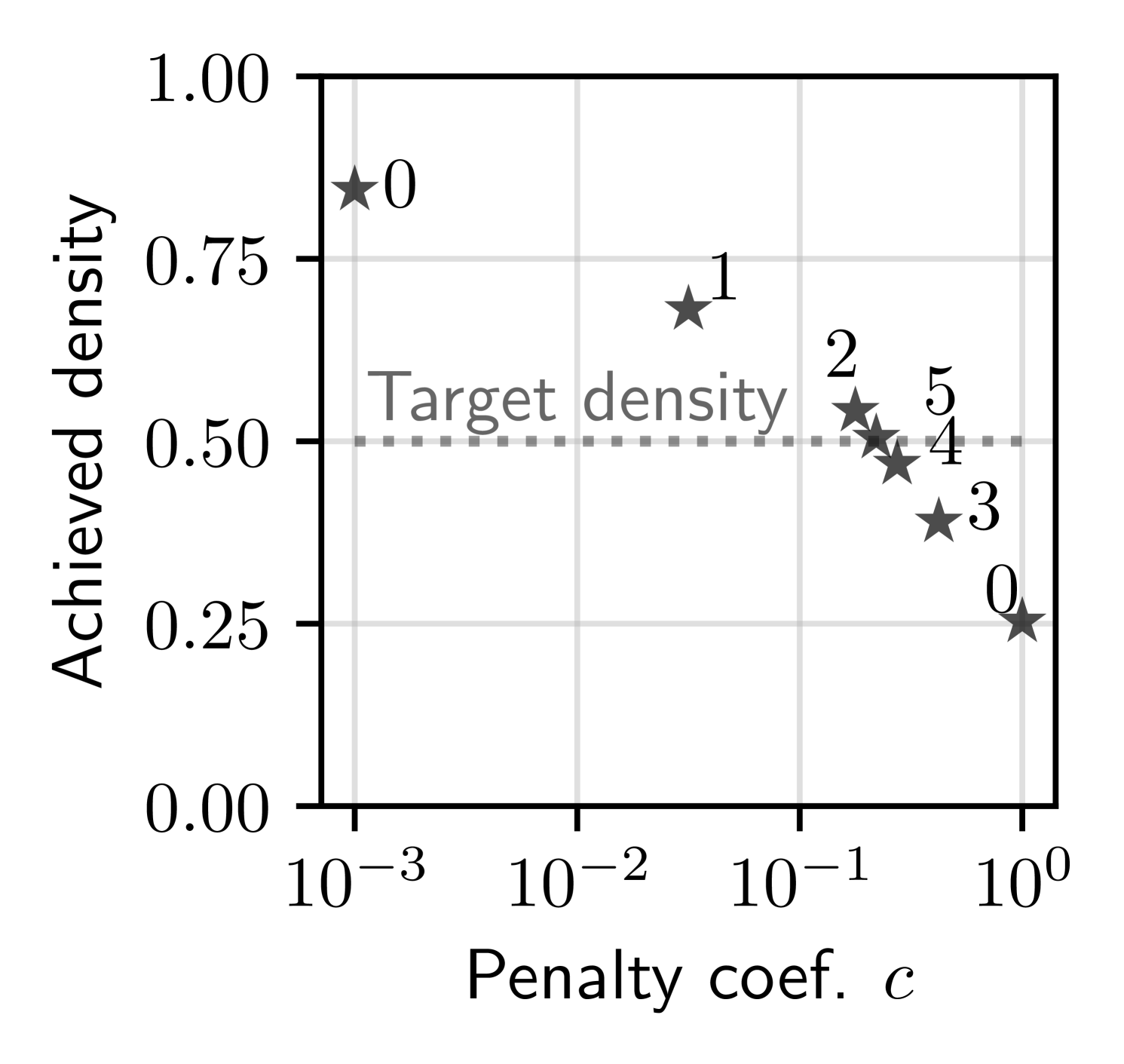
The unnecessarily lengthy process of tuning penalty coefficients is illustrated in Fig.˜1, where the goal is to train a neural network under a constraint enforcing at least sparsity. Using bisection search—which leverages the monotonic relationship between the coefficient and the resulting constraint value—the penalized problem must be solved five times before finding a satisfactory solution: one that is feasible but not overly sparse, as excessive sparsity would degrade performance. Even with this simple tuning method, the example demonstrates the process’s inefficiency. In contrast, a proper constrained optimization method can solve the problem in one shot, requiring only a single model training run (Gallego-Posada et al., 2022).
Several factors make coefficient tuning challenging: \raisebox{-.7pt}{{\hspace{-0.8mm} \small1}}⃝ The relationship between a given coefficient and the resulting values of , , and is often highly non-linear, requiring specialized hyperparameter tuning techniques or even manual intervention; \raisebox{-.7pt}{{\hspace{-0.8mm} \small2}}⃝ Penalty coefficients lack intuitive semantics, making them difficult to interpret; and \raisebox{-.7pt}{{\hspace{-0.8mm} \small3}}⃝ There is no general principled strategy for initializing them.
In contrast, constraint levels in constrained formulations \raisebox{-.7pt}{{\hspace{-0.8mm} \small1}}⃝ map directly to constraint values and \raisebox{-.7pt}{{\hspace{-0.8mm} \small2}}⃝ are interpretable, since their units match those of the constraints. In constrained approaches that learn the “coefficients”—e.g., the multipliers in the Lagrangian approach—\raisebox{-.7pt}{{\hspace{-0.8mm} \small3}}⃝ initialization is less critical, as they adapt during optimization and are thus typically set to zero for simplicity.
Moreover, tuning penalty coefficients becomes increasingly impractical in the presence of multiple constraints, and is further complicated by the fact that coefficient choices rarely transfer across tasks.
Multiple constraints. Tuning penalty coefficients becomes substantially more difficult in the presence of multiple constraints. Unlike the single-constraint case, multiple coefficients must be tuned jointly, as each one influences the satisfaction of all constraints. Moreover, while the monotonic relationship between coefficients and constraint values is straightforward to exploit in the single-constraint setting (e.g., as demonstrated in Fig.˜1), extending this to the multi-constraint setting is challenging. This interdependence significantly increases the complexity of the tuning process, often rendering it impractical and potentially leading practitioners to accept suboptimal—or even infeasible—solutions.
Penalty coefficients rarely transfer across settings. The same coefficient can yield different outcomes across architectures and datasets, due to changes in the landscape of the penalized objective. Moreover, adding new constraints to an existing problem typically requires re-tuning all coefficients, as feasibility may depend on rebalancing them to account for both existing and new constraints.
In contrast, the hyperparameters of the constrained approach—the constraint levels and —are agnostic to the number of constraints, their parameterization, or their relationship to model inputs. While some constrained methods may still require hyperparameter tuning when tasks change or new constraints are added, these typically transfer more reliably than penalty coefficients (see §4.2).
4 Getting started with constrained learning: the Lagrangian approach
We adopt the Lagrangian approach (Arrow et al., 1958) to illustrate how a principled non-convex constrained optimization method addresses the limitations of the penalized approach. We choose this approach because of its broad applicability (requiring only differentiability), its similarity to penalized methods (facilitating comparison), its widespread use for (principled) constrained deep learning (Gallego-Posada, 2024), and the limited repertoire of methods for large-scale non-convex constrained optimization (see §5 for details).
4.1 The Lagrangian approach
The Lagrangian approach (Arrow et al., 1958) amounts to finding stationary points of the Lagrangian, which may correspond to solutions of the original constrained optimization problem (see §2):
| (7) |
This reformulates the constrained problem as an effectively unconstrained777Given that can be easily handled via projections. optimization problem. Notably, the Lagrangian is always linear—and therefore concave—in the multipliers.
A simple algorithm for finding stationary points of is alternating gradient descent–ascent (GDA):
| (8) | ||||
| (9) | ||||
| (10) |
where denotes a projection onto to enforce , denotes a projection onto , and are step-sizes. The multipliers are typically initialized as and . We favor alternating updates over simultaneous ones due to their enhanced convergence guarantees under a strongly convex (Zhang et al., 2022), without incurring additional computational cost on Lagrangian games (Sohrabi et al., 2024).
Note that the update with respect to in Eq.˜8 matches that of (projected) gradient descent on the penalized objective, with and . However, unlike penalty coefficients, which require manual tuning, the multipliers are instead optimized to balance feasibility and optimality.
The Lagrangian approach has been successfully applied to a wide range of constrained deep learning problems (Cotter et al., 2019b; Hashemizadeh et al., 2024; Gallego-Posada et al., 2022; Robey et al., 2021; Stooke et al., 2020; Elenter et al., 2022; Hounie et al., 2023b; Dai et al., 2024; Hounie et al., 2023a; Ramirez et al., 2025). Beyond this effectiveness, it is also viable in practice, as discussed below.
Dynamics of GDA. Consider a single inequality constraint . The corresponding dual variable is updated based on the constraint violation: when , increases by . Repeated violations drive larger, which shifts the primal update toward reducing and promoting feasibility. Conversely, when , decreases. In turn, a smaller multiplier shifts focus away from constraint satisfaction and toward minimizing the objective. When , the constraint is ignored. For instance, consider a classification problem with a sparsity constraint. When the number of non-zero parameters exceeds the constraint level, the multiplier increases, pushing the model to be sparser. For an equality constraint , the multiplier increases when . Conversely, it decreases—becoming negative—when . These dynamics encourage to approach .
Computational cost. Applying (mini-batch) GDA to the Lagrangian is as efficient as applying (mini-batch) GD to the penalized objective , since the primal updates in both cases follow a linear combination of the objective and constraint gradients. The only overhead is updating the multipliers, which is negligible when the number of constraints is much smaller than .
Tuning . A larger dual step-size makes the multipliers respond more aggressively to constraint violations: if is too small, constraints may remain unsatisfied within the optimization budget; if too large, rapidly growing multipliers can overshoot their targets and . In practice, however, tuning is significantly easier than tuning penalty coefficients—a point we elaborate on in §4.2.
Implementation. The Lagrangian approach is straightforward to implement in popular deep learning frameworks such as PyTorch (Paszke et al., 2019) and JAX (Bradbury et al., 2018). Open-source libraries like Cooper (Gallego-Posada et al., 2025) for PyTorch and TFCO (Cotter et al., 2019c) for TensorFlow (Abadi et al., 2016) offer ready-to-use implementations, along with additional features such as the Augmented Lagrangian (Bertsekas, 1975), Proxy Constraints (Cotter et al., 2019b), Multiplier Models (Narasimhan et al., 2020), and PI (Sohrabi et al., 2024).
Convergence. If is strongly convex in , Eq.˜7 becomes a strongly convex–concave min–max problem, for which alternating GDA enjoys local linear convergence (Zhang et al., 2022). Moreover, simultaneous GDA converges to local min–max points in non-convex–concave settings, provided the maximization domain is compact (Lin et al., 2025). While the domains of and are unbounded, if the optimal multipliers are finite, restricting optimization to a bounded region containing them allows these guarantees to hold.
Generalization. Chamon and Ribeiro (2020) develop a PAC learning framework for constrained learning. They argue that hypothesis classes that are PAC-learnable in the unconstrained setting may remain learnable under statistical constraints, probably approximately satisfying them on unseen data.
4.2 Contrasting the Lagrangian and penalized approaches
This section elaborates on why the simple Lagrangian approach is, in many respects, preferable to the penalized formulation. In short, transitioning to the Lagrangian approach—which can be seen as a principled alternative to manually tuning penalty coefficients by instead increasing them when constraints are violated and decreasing them when satisfied—yields an algorithm that: \raisebox{-.7pt}{{\hspace{-0.8mm} \small1}}⃝ is explicitly designed to solve the constrained problem, and is therefore expected to do so; and \raisebox{-.7pt}{{\hspace{-0.8mm} \small2}}⃝ requires substantially less manual hyperparameter tuning. As discussed in §4.3, it also offers several additional benefits, many of which remain relatively underexplored in the deep learning literature.
The Lagrangian approach is constrained by design. Lagrangian optimization continues until a feasible solution is found. In contrast, the penalized approach may converge while still producing an infeasible solution. This constrained-by-design philosophy also introduces a notion of accountability: by explicitly specifying acceptable values for and in the formulation, we adopt a more principled framework for both solving the problem and evaluating success—where infeasibility is not acceptable.
The Lagrangian approach can solve non-convex problems. As shown in Table˜1 (App. C.1), the Lagrangian approach successfully recovers the correct solution to Example˜1. Note that this requires either a specialized dual optimizer such as PI (Sohrabi et al., 2024), or the Augmented Lagrangian method; standard gradient descent-ascent fails in this setting due to the concavity of the Lagrangian with respect to . PI overcomes this by dampening the oscillations that arise with GDA, while the Augmented Lagrangian method convexifies the problem—both enabling convergence to the constrained optimum (see App. D for details). Hyperparameter choices for Table˜1 are provided in App. B.1.
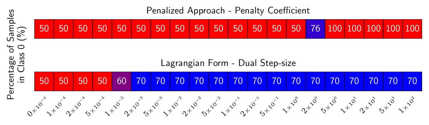
Hyperparameter tuning. The Lagrangian approach eliminates the need to tune penalty coefficients, but introduces a complementary challenge: selecting the dual step-size . However, this tuning is generally more forgiving—whereas typically only a single choice of penalty coefficient yields a satisfactory solution, a broad range of dual step-sizes often leads to feasibility, sometimes spanning several orders of magnitude. This is because the Lagrangian approach always pursues constraint satisfaction—regardless of how aggressively, as determined by the step-size—unlike the penalized approach, which is agnostic to the constraint levels. For this reason, we argue that this relative ease of tuning likely extends to other constrained optimization methods beyond the Lagrangian approach.
Figure˜2 illustrates this on a rate-constrained binary classification task (Cotter et al., 2019b), where 70% of predictions are required to belong to class “0”. Since the data is balanced, the optimal constrained solution should assign 70% of predictions to class 0—this is achieved with an optimal Lagrange multiplier of , as found experimentally via the Lagrangian approach. The penalized formulation is infeasible for all ; for , it satisfies the constraint but collapses to predicting a single class, degrading performance. Only at does it yield a reasonable prediction rate of 76%. In contrast, the Lagrangian approach with proxy constraints (Cotter et al., 2019b) consistently recovers the correct solution over a wide range of dual step-sizes by automatically learning the appropriate multiplier (see App. B.3).
4.3 Further benefits of the Lagrangian approach
Recent advances in constrained learning have equipped the Lagrangian approach with new capabilities that further strengthen its appeal in deep learning applications.
Non-differentiable constraints. Cotter et al. (2019b) show that the Lagrangian approach can be extended to satisfy non-differentiable constraints by using a differentiable surrogate during the primal update—where constraint gradients are required—while relying on the original, non-differentiable constraint when updating the multipliers. This “proxy constraints” approach ensures that constraint enforcement is driven by the true quantity of interest, independent of the choice of surrogate.
This capability is particularly relevant in machine learning, where optimization often relies on differentiable surrogates that do not match the true objective. While unconstrained empirical risk minimization offers no direct way to optimize for accuracy—e.g., optimizing cross-entropy instead—accuracy-based constraints can be enforced via the Lagrangian formulation with proxy constraints (Cotter et al., 2019b; Hashemizadeh et al., 2024).
Scaling the number of constraints. Each additional constraint introduces one more Lagrange multiplier—a single scalar. While this already scales efficiently, especially given the Lagrangian approach’s greater robustness to hyperparameters compared to the penalized formulation (§4.2), scalability can be further improved using parametric Lagrange multiplier models (Narasimhan et al., 2020). These models use a fixed set of parameters to represent all multipliers, regardless of the number of constraints, and can thus handle even problems with infinitely many constraints—unlike the penalized approach.
Sensitivity analysis via the multipliers. A standard result states that the optimal Lagrange multipliers and capture how much the objective would improve if a constraint were relaxed (Boyd and Vandenberghe, 2004, §5.6). This can be exploited to design algorithms that trade off constraint tightness for performance (Hounie et al., 2024), making the Lagrangian approach well suited to settings with flexible or uncertain constraint levels.
Efficient dual variance reduction. Variance reduction techniques (Gower et al., 2020), popular for accelerating convergence in unconstrained optimization, have seen limited adoption in deep learning due to poor scalability—e.g., SAGA (Defazio et al., 2014) requires storing gradients for each datapoint. In contrast, they are inexpensive to apply to Lagrange multiplier updates, as the dual gradient is simply the constraint value, and have been shown to enhance convergence for problems involving stochastic constraints (Hashemizadeh et al., 2024).
Hyperparameter scaling. We hypothesize that, for a given task, the choice of dual step-sizes transfers well across model architectures and datasets. This would make hyperparameter scaling in the constrained approach significantly easier—allowing practitioners to tune parameters on smaller models and reuse them as effective starting points for larger-scale training, saving time and resources.
5 Call for research: enhancing constrained deep learning
Constrained learning still has notable limitations. This section reviews the key challenges and seeks to spur further research on tailored constrained deep learning algorithms.
Choosing the constraint levels and . Domain knowledge often informs acceptable constraint levels; however these are sometimes unclear. If set too tightly, the problem may become infeasible; if too loose, the desired properties may be weakly enforced. In non-convex settings, it is often unclear whether the levels are overly strict or too lax. This can be mitigated by introducing slack variables that adjust constraint levels to balance the objective and constraints (Hounie et al., 2024). However, when no meaningful levels can be specified, tailored multi-objective optimization methods may be more appropriate.
Limited repertoire of methods for constrained deep learning. The non-convexity of the feasible set in Eq.˜1 rules out standard methods such as projected gradient descent (Goldstein, 1964; Levitin and Polyak, 1966; Bertsekas, 1976) and feasible direction methods (Frank and Wolfe, 1956; Zoutendijk, 1960), as computing projections or feasible directions over non-convex sets is often intractable. Methods that require all iterates to remain feasible, such as barrier methods (Dikin, 1967), also break down in practice when constraints are estimated from mini-batches, due to variability in feasibility assessment across batches. The scale of deep learning further limits practical options: for example, vanilla SQPs (Wilson, 1963; Han, 1977; Powell, 1978) incur a per-iteration cost of , which is prohibitive for large models. Penalty methods such as the quadratic penalty method (Nocedal and Wright, 2006, §17.1) remain applicable, but often require excessively large penalty coefficients to succeed—leading to numerical instability.
While the Lagrangian (Arrow et al., 1958) and Augmented Lagrangian (Bertsekas, 1975) approaches remain applicable—both reformulating constrained problems as min-max games—they still face challenges:
Non-existence of optimal Lagrange multipliers. A necessary and sufficient condition for the existence of finite optimal Lagrange multipliers satisfying the KKT conditions at in differentiable problems is the Mangasarian–Fromovitz constraint qualification (MFCQ) (Mangasarian and Fromovitz, 1967; Gauvin, 1977). However, when MFCQ fails, the Lagrangian and Augmented Lagrangian approaches do not necessarily break down. Convergence to can still be achieved approximately by allowing or (see §2 for details). Although large multipliers may lead to numerical instability when optimizing for , many problems still admit approximate constrained minimizers that are sufficiently close to without requiring excessively large multipliers.
Thus, the failure of MFCQ does not necessarily make the Lagrangian approach ill-posed. However, it does limit the effectiveness of dual updates via gradient ascent. As primal iterates approach feasibility and constraint violations decrease, the dual updates tend to slow and may eventually stall—causing the multipliers to plateau before they have fully closed the feasibility gap.
Optimization. The min-max structure of the Lagrangian formulation can induce oscillations in the multipliers and their associated constraints, slowing convergence—an issue further exacerbated by dual momentum (Sohrabi et al., 2024). These oscillations can be mitigated using PI controllers on the multipliers (Stooke et al., 2020; Sohrabi et al., 2024) or by the Augmented Lagrangian approach (Platt and Barr, 1987). However, both methods introduce additional hyperparameters: the damping coefficient in the former and the penalty coefficient in the latter.
While helpful in practice, tuning these additional hyperparameters remains challenging. Even setting the dual step-size—though much easier than tuning penalty coefficients—remains a burden. Ideally, we would develop self-tuning strategies for updating dual variables, akin to Adam (Kingma and Ba, 2015) in non-convex unconstrained minimization, that work reliably out of the box across a broad range of problems.
Generalization. When constraints depend on data, satisfying them on the training set does not guarantee feasibility on unseen samples. Despite PAC guarantees (Chamon and Ribeiro, 2020), constraint satisfaction often fails to generalize in practice (Cotter et al., 2019a; Hashemizadeh et al., 2024). Cotter et al. (2019a) propose a regularization strategy that uses a held-out set to train the multipliers, while updating the model parameters using the main training set. This decouples the signal enforcing constraint satisfaction (the multipliers) from the signal responsible for achieving it (the model), helping prevent the model from overfitting to the constraints. Nonetheless, exploring additional regularization strategies remains an important research direction.
6 Conclusion
Recent efforts to build trustworthy and safe AI systems with accountability guarantees have led to a growing focus on constrained optimization in deep learning. We argue against penalized approaches for solving such problems, due to their unreliability and the difficulty of tuning them—especially in settings where domain knowledge prescribes desirable constraint levels, making the constrained formulation both natural and principled. We also identify open research directions for constrained deep learning methods which—building on their success in large-scale, non-convex problems—offer opportunities to further enhance their optimization adaptability and generalization performance.
Broader Impact Statement
This paper is pertinent to nearly all machine learning practitioners, not just a niche sub-community. This is because researchers and practitioners very frequently encounter tasks requiring the enforcement of multiple properties. Through this work, we aim to enhance the entire community’s toolkit by providing more robust methods for addressing these problems, beyond the flawed penalized approach. Moving beyond the penalized approach offers significant advantages, such as:
-
•
Achieving better objective-constraint trade-offs: This would enable practitioners to reach trade-offs that were previously out of reach. As a result, techniques or models that were once discarded for failing to meet desired requirements could become viable.
-
•
Reducing tuning overhead: It would lessen the time and resources spent tuning penalty coefficients, which is a major burden on the machine learning community. This also lowers the computational footprint linked to repeated model training during hyperparameter searches.
-
•
Spurring further research: Broader adoption of constrained methods would motivate more research into constrained learning. This would lead to the development of more effective and efficient algorithms, which would, in turn, further benefit the community.
Acknowledgements and disclosure of funding
This work was supported by the Canada CIFAR AI Chair program (Mila), the NSERC Discovery Grant RGPIN-2025-05123, by an unrestricted gift from Google, and by Samsung Electronics Co., Ldt. Simon Lacoste-Julien is a CIFAR Associate Fellow in the Learning in Machines & Brains program.
We thank Jose Gallego-Posada and Lucas Maes for their helpful discussions during the conceptualization of this work.
Many of the ideas presented in this work arose from discussions during the development of various research papers on constrained deep learning. This is especially true for Gallego-Posada et al. (2022). We would therefore like to thank our collaborators Yoshua Bengio, Juan Elenter, Akram Erraqabi, Jose Gallego-Posada, Golnoosh Farnadi, Ignacio Hounie, Alejandro Ribeiro, Rohan Sukumaran, Motahareh Sohrabi, and Tianyue (Helen) Zhang.
References
- Abadi et al. (2016) M. Abadi et al. TensorFlow: A system for Large-Scale machine learning. In 12th USENIX Symposium on Operating Systems Design and Implementation (OSDI 16), 2016.
- Arrow et al. (1958) K. Arrow, L. Hurwicz, and H. Uzawa. Studies in Linear and Non-linear Programming. Stanford University Press, 1958.
- Bachute and Subhedar (2021) M. R. Bachute and J. M. Subhedar. Autonomous Driving Architectures. Machine Learning with Applications, 2021.
- Bertsekas (1975) D. Bertsekas. On the Method of Multipliers for Convex Programming. IEEE Transactions on Automatic Control, 1975.
- Bertsekas (2016) D. Bertsekas. Nonlinear Programming. Athena Scientific, 2016.
- Bertsekas (1976) D. P. Bertsekas. On the Goldstein-Levitin-Polyak Gradient Projection Method. IEEE Transactions on automatic control, 1976.
- Bhatore et al. (2020) S. Bhatore et al. Machine learning techniques for credit risk evaluation. Journal of Banking and Financial Technology, 2020.
- Birgin and Mart´ınez (2014) E. G. Birgin and J. M. Martínez. Practical Augmented Lagrangian Methods for Constrained Optimization. The SIAM series on Fundamentals of Algorithms, 2014.
- Boyd and Vandenberghe (2004) S. Boyd and L. Vandenberghe. Convex Optimization. Cambridge University Press, 2004.
- Bradbury et al. (2018) J. Bradbury et al. JAX: composable transformations of Python+NumPy programs. http://github.com/google/jax, 2018.
- Brouillard et al. (2020) P. Brouillard, S. Lachapelle, A. Lacoste, S. Lacoste-Julien, and A. Drouin. Differentiable Causal Discovery from Interventional Data. In NeurIPS, 2020.
- Chakraborty et al. (2025) D. Chakraborty, Y. LeCun, T. G. Rudner, and E. Learned-Miller. Improving Pre-trained Self-Supervised Embeddings Through Effective Entropy Maximization. In AISTATS, 2025.
- Chamon and Ribeiro (2020) L. Chamon and A. Ribeiro. Probably Approximately Correct Constrained Learning. In NeurIPS, 2020.
- Chen et al. (2016) X. Chen, Y. Duan, R. Houthooft, J. Schulman, I. Sutskever, and P. Abbeel. InfoGAN: Interpretable Representation Learning by Information Maximizing Generative Adversarial Nets. In NeurIPS, 2016.
- Cotter et al. (2019a) A. Cotter, M. Gupta, H. Jiang, N. Srebro, K. Sridharan, S. Wang, B. Woodworth, and S. You. Training Well-Generalizing Classifiers for Fairness Metrics and Other Data-Dependent Constraints. In ICML, 2019a.
- Cotter et al. (2019b) A. Cotter, H. Jiang, M. R. Gupta, S. Wang, T. Narayan, S. You, and K. Sridharan. Optimization with Non-Differentiable Constraints with Applications to Fairness, Recall, Churn, and Other Goals. JMLR, 2019b.
- Cotter et al. (2019c) A. Cotter et al. TensorFlow Constrained Optimization (TFCO). https://github.com/ google-research/tensorflow_constrained_optimization, 2019c.
- Dahl et al. (2023) G. E. Dahl, F. Schneider, Z. Nado, N. Agarwal, C. S. Sastry, P. Hennig, S. Medapati, R. Eschenhagen, P. Kasimbeg, D. Suo, J. Bae, J. Gilmer, A. L. Peirson, B. Khan, R. Anil, M. Rabbat, S. Krishnan, D. Snider, E. Amid, K. Chen, C. J. Maddison, R. Vasudev, M. Badura, A. Garg, and P. Mattson. Benchmarking Neural Network Training Algorithms. arXiv preprint arXiv:2306.07179, 2023.
- Dai et al. (2024) J. Dai, X. Pan, R. Sun, J. Ji, X. Xu, M. Liu, Y. Wang, and Y. Yang. Safe RLHF: Safe Reinforcement Learning from Human Feedback. In ICLR, 2024.
- Defazio et al. (2014) A. Defazio, F. Bach, and S. Lacoste-Julien. SAGA: A Fast Incremental Gradient Method With Support for Non-Strongly Convex Composite Objectives. In NeurIPS, 2014.
- Degrave and Korshunova (2021a) J. Degrave and I. Korshunova. Why machine learning algorithms are hard to tune and how to fix it. Engraved, blog: www.engraved.blog/why-machine-learning-algorithms-are-hard-to-tune/, 2021a.
- Degrave and Korshunova (2021b) J. Degrave and I. Korshunova. How we can make machine learning algorithms tunable. Engraved, blog: www.engraved.blog/how-we-can-make-machine-learning-algorithms-tunable/, 2021b.
- Dikin (1967) I. I. Dikin. Iterative Solution of Problems of Linear and Quadratic Programming. In Doklady Akademii Nauk. Russian Academy of Sciences, 1967.
- Dilhac et al. (2018) M.-A. Dilhac et al. Montréal Declaration for a Responsible Development of Artificial Intelligence, 2018.
- Dunion et al. (2023) M. Dunion, T. McInroe, K. Luck, J. Hanna, and S. Albrecht. Conditional Mutual Information for Disentangled Representations in Reinforcement Learning. In NeurIPS, 2023.
- Ehrgott (2005) M. Ehrgott. Multicriteria Optimization. Springer Science & Business Media, 2005.
- Elenter et al. (2022) J. Elenter, N. NaderiAlizadeh, and A. Ribeiro. A Lagrangian Duality Approach to Active Learning. In NeurIPS, 2022.
- European Parliament (2024) European Parliament. Artificial Intelligence Act. https://artificialintelligenceact.eu, 2024.
- Frank and Wolfe (1956) M. Frank and P. Wolfe. An Algorithm for Quadratic Programming. Naval Research Logistics Quarterly, 1956.
- Gallego-Posada (2024) J. Gallego-Posada. Constrained Optimization for Machine Learning: Algorithms and Applications. PhD Thesis, University of Montreal, 2024.
- Gallego-Posada et al. (2022) J. Gallego-Posada, J. Ramirez, A. Erraqabi, Y. Bengio, and S. Lacoste-Julien. Controlled Sparsity via Constrained Optimization or: How I Learned to Stop Tuning Penalties and Love Constraints. In NeurIPS, 2022.
- Gallego-Posada et al. (2025) J. Gallego-Posada, J. Ramirez, M. Hashemizadeh, and S. Lacoste-Julien. Cooper: A Library for Constrained Optimization in Deep Learning. arXiv preprint arXiv:2504.01212, 2025.
- Gauvin (1977) J. Gauvin. A Necessary and Sufficient Regularity Condition to Have Bounded Multipliers in Nonconvex Programming. Mathematical Programming, 1977.
- Gemini Team (2024) Gemini Team. Gemini 1.5: Unlocking multimodal understanding across millions of tokens of context. arXiv preprint arXiv:2403.05530, 2024.
- Goldstein (1964) A. A. Goldstein. Convex Programming in Hilbert Space. University of Washington, 1964.
- Gower et al. (2020) R. M. Gower, M. Schmidt, F. Bach, and P. Richtárik. Variance-Reduced Methods for Machine Learning. Proceedings of the IEEE, 2020.
- Han (1977) S.-P. Han. A globally convergent method for nonlinear programming. Journal of optimization theory and applications, 1977.
- Hashemizadeh et al. (2024) M. Hashemizadeh, J. Ramirez, R. Sukumaran, G. Farnadi, S. Lacoste-Julien, and J. Gallego-Posada. Balancing Act: Constraining Disparate Impact in Sparse Models. In ICLR, 2024.
- Higgins et al. (2017) I. Higgins, L. Matthey, A. Pal, C. Burgess, X. Glorot, M. Botvinick, S. Mohamed, and A. Lerchner. beta-VAE: Learning Basic Visual Concepts with a Constrained Variational Framework . In ICLR, 2017.
- Hounie et al. (2023a) I. Hounie, L. F. Chamon, and A. Ribeiro. Automatic Data Augmentation via Invariance-Constrained Learning. In ICML, 2023a.
- Hounie et al. (2023b) I. Hounie, J. Elenter, and A. Ribeiro. Neural Networks with Quantization Constraints. In ICASSP, 2023b.
- Hounie et al. (2024) I. Hounie, A. Ribeiro, and L. F. Chamon. Resilient Constrained Learning. In NeurIPS, 2024.
- Kingma and Ba (2015) D. Kingma and J. Ba. Adam: A Method for Stochastic Optimization. In ICLR, 2015.
- Kumar et al. (2018) A. Kumar, P. Sattigeri, and A. Balakrishnan. Variational Inference of Disentangled Latent Concepts from Unlabeled Observations. In ICLR, 2018.
- Larson et al. (2016) J. Larson et al. Data and analysis for “Machine Bias”. https://github.com/propublica/compas-analysis, 2016.
- Levitin and Polyak (1966) E. S. Levitin and B. T. Polyak. Constrained Minimization Methods. USSR Computational mathematics and mathematical physics, 1966.
- Lin et al. (2025) T. Lin, C. Jin, and M. I. Jordan. Two-Timescale Gradient Descent Ascent Algorithms for Nonconvex Minimax Optimization. JMLR, 2025.
- Louizos et al. (2018) C. Louizos, M. Welling, and D. P. Kingma. Learning Sparse Neural Networks through Regularization. In ICLR, 2018.
- Mangasarian and Fromovitz (1967) O. L. Mangasarian and S. Fromovitz. The Fritz John Necessary Optimality Conditions in the Presence of Equality and Inequality Constraints. Journal of Mathematical Analysis and Applications, 1967.
- Miettinen (1999) K. Miettinen. Nonlinear Multiobjective Optimization. Springer Science & Business Media, 1999.
- Narasimhan et al. (2020) H. Narasimhan, A. Cotter, Y. Zhou, S. Wang, and W. Guo. Approximate Heavily-Constrained Learning with Lagrange Multiplier Models. In NeurIPS, 2020.
- Nocedal and Wright (2006) J. Nocedal and S. J. Wright. Numerical Optimization. Springer, 2006.
- OpenAI (2023) OpenAI. GPT-4 Technical Report. arXiv preprint arXiv:2303.08774, 2023.
- Paszke et al. (2019) A. Paszke et al. PyTorch: An Imperative Style, High-Performance Deep Learning Library. In NeurIPS, 2019.
- Platt and Barr (1987) J. C. Platt and A. H. Barr. Constrained Differential Optimization. In NeurIPS, 1987.
- Powell (1978) M. J. Powell. The convergence of variable metric methods for nonlinearly constrained optimization calculations. In Nonlinear programming 3. Elsevier, 1978.
- Ramirez et al. (2025) J. Ramirez, I. Hounie, J. Elenter, J. Gallego-Posada, M. Hashemizadeh, A. Ribeiro, and S. Lacoste-Julien. Feasible Learning. In AISTATS, 2025.
- Robey et al. (2021) A. Robey, L. Chamon, G. J. Pappas, H. Hassani, and A. Ribeiro. Adversarial Robustness with Semi-Infinite Constrained Learning. In NeurIPS, 2021.
- Shi et al. (2025) E. Shi, L. Kong, and B. Jiang. Deep Fair Learning: A Unified Framework for Fine-tuning Representations with Sufficient Networks. arXiv preprint arXiv:2504.06470, 2025.
- Sohrabi et al. (2024) M. Sohrabi, J. Ramirez, T. H. Zhang, S. Lacoste-Julien, and J. Gallego-Posada. On PI Controllers for Updating Lagrange Multipliers in Constrained Optimization. In ICML, 2024.
- Stooke et al. (2020) A. Stooke, J. Achiam, and P. Abbeel. Responsive Safety in Reinforcement Learning by PID Lagrangian Methods. In ICML, 2020.
- Wilson (1963) R. B. Wilson. A simplicial algorithm for concave programming. PhD Thesis, Graduate School of Bussiness Administration, 1963.
- Zhang et al. (2022) G. Zhang, Y. Wang, L. Lessard, and R. B. Grosse. Near-optimal Local Convergence of Alternating Gradient Descent-Ascent for Minimax Optimization. In AISTATS, 2022.
- Zhu et al. (2017) J.-Y. Zhu, T. Park, P. Isola, and A. A. Efros. Unpaired Image-to-Image Translation using Cycle-Consistent Adversarial Networks. In ICCV, 2017.
- Zoutendijk (1960) G. Zoutendijk. Methods of Feasible Directions: A Study in Linear and Non-linear Programming. Elsevier Publishing Company, 1960.
Appendix A Proofs
Proof of Proposition 1.
Since is a regular constrained minimizer with corresponding optimal Lagrange multipliers and , we can invoke the KKT conditions, which state:
| (11) |
Choose and . The stationarity condition then implies that is a critical point of the penalized objective
The objective is convex in , as it is the sum of the convex function , the convex function , and the affine function . For convex functions, any critical point is a global minimizer. Hence,
∎
Proof of Proposition 2.
We first show that the point satisfies the first-order necessary conditions for constrained optimality.
We verify the KKT conditions:
-
1.
Primal feasibility. We have .
-
2.
Stationarity. The gradients of with respect to the primal variables vanish at :
(13) (14) -
3.
Complementary slackness. We have . Since , strict complementary slackness holds.
We now verify that satisfies the second-order sufficient conditions for optimality [Bertsekas, 2016, Prop. 4.3.2]. Consider the Hessian of with respect to :
| (15) |
At , this becomes:
| (16) |
To satisfy the second-order sufficient conditions, we must ensure that the Hessian is positive definite on the null space of constraints at —that is, the set of feasible first-order directions that preserve the set of active constraints.
The gradient of the active constraint is:
| (17) |
Thus, the null space is:
| (18) |
For any :
| (19) |
Since the Hessian is (strictly) positive definite over , and satisfies the first-order conditions along with strict complementary slackness, it follows that is a strict local constrained minimizer of Example˜1.
Substituting the solution, we find:
To verify global optimality, we evaluate the objective and constraint at the boundaries of the domain:
-
•
At , the constraint evaluates to , which is infeasible.
-
•
At , we have , and the objective becomes , which is minimized at , giving .
However, , so we conclude that is the global constrained minimizer of Example˜1.
∎
Proof of Proposition 3.
We begin by factorizing the penalized objective as:
Since for and , the minimum with respect to is attained at . Let , and compute its derivatives:
| (20) | ||||
| (21) |
Thus, is strictly concave on the interval. While its maximum occurs at the critical point , we are minimizing , so the minimizer must lie at one of the boundaries.
-
•
For , we have , so the minimum is at .
-
•
For , we have , so the minimum is at .
-
•
When , both endpoints yield the same value: .
Evaluating the constraint and objective at the endpoints, we find: , ; and , . ∎
Appendix B Experimental Details
Our implementations use PyTorch [Paszke et al., 2019] and the Cooper library for constrained deep learning [Gallego-Posada et al., 2025]. Our code is available at: https://github.com/merajhashemi/constraints-vs-penalties.
B.1 Example 1
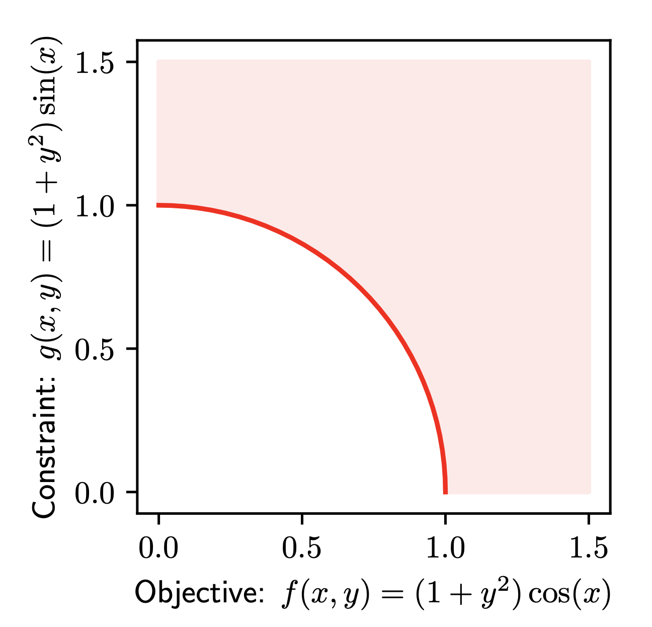
Figure˜3 illustrates the Pareto front of non-dominated solutions to Example˜1. Varying changes the angle (position) of a point along the Pareto front, while varying controls its distance from the front. Intuitively, this shows that all optimal solutions occur at . Moreover, imposing a constraint of the form restricts the optimization of to the region below the line ; since minimizing with respect to requires increasing , this constraint selects a specific solution on the front where . The choice of therefore determines the corresponding optimal value of , that is, the position along the front.
Intuitively, the concavity of this Pareto front—which is tied to the concavity of the penalized function for this problem—causes gradient descent on the penalized objective to fall to the corners of the front. In contrast, a convex Pareto front—which would arise under the convexity assumptions outlined in Prop.˜1—would allow gradient descent to reach intermediate points, enabling proper exploration of the trade-offs between and by varying .
See Degrave and Korshunova [2021a, b] for animations illustrating the optimization dynamics of \raisebox{-.7pt}{{\hspace{-0.8mm} \small1}}⃝ gradient descent on the penalized formulation, which falls to the corners; \raisebox{-.7pt}{{\hspace{-0.8mm} \small2}}⃝ gradient descent-ascent on the Lagrangian, which oscillates without converging; \raisebox{-.7pt}{{\hspace{-0.8mm} \small3}}⃝ and gradient descent-ascent on the Augmented Lagrangian, which does converge.
Hyper-parameters. We use the Lagrangian approach to solve Example˜1, applying gradient descent with a step-size of as the primal optimizer and PI [Sohrabi et al., 2024]—as implemented in Cooper [Gallego-Posada et al., 2025]—as the dual optimizer, with a step-size of , damping coefficient , and . To enforce , we apply a projection after every primal update. Table˜1 in Section˜C.1 presents results after 10,000 training iterations. We elaborate on this choice of dual optimizer in Appendix˜D—it is necessary for convergence, as standard gradient ascent would otherwise lead to undamped oscillations.
B.2 Sparsity Constraints
Louizos et al. [2018] propose a model reparameterization that enables applying -norm regularization to the weights via stochastic gates that follow a Hard Concrete distribution parameterized by . This is formulated in a penalized fashion as follows:
| (22) |
where are the model parameters, is the task loss, is the dataset, denotes the norm, and is a penalty coefficient.
To illustrate the tunability advantages of constrained approaches over the penalized approach, we replicate the bisection search experiment from Figure 5(b), Appendix E of Gallego-Posada et al. [2022]. We use their MNIST classification setup with an MLP (300–100 hidden units), as shown in Fig.˜1. To achieve 50% global sparsity, we perform a log-scale bisection search over penalty coefficients. The corresponding results, including model training accuracy, are reported in Table˜2 in Section˜C.2.
Akin to Gallego-Posada et al. [2022], we set the temperature of the stochastic gate distribution to and use a stretching interval of . The droprate init is set to , resulting in a fully dense model at the start of training. We use Adam [Kingma and Ba, 2015] with a step-size of for optimizing both the model and gate parameters. Training is performed for epochs with a batch size of .
B.3 Rate Constraints
We consider a linear binary classification problem , where the model is constrained to predict class 0 for at least 70% of the training examples. The resulting optimization problem is:
| (23) |
where denotes the cross-entropy loss, and are the weights and bias of the linear model, are input-label pairs drawn from the data distribution , and is the sigmoid function.
This rate-constrained setup matches the experiment in Figure 2 of Cotter et al. [2019b], originally designed to showcase the effectiveness of their method for handling non-differentiable constraints. Here, we repurpose it to highlight the tunability advantages of the Lagrangian approach over the penalized one.
Since the constraint is not differentiable with respect to the model parameters, we follow Cotter et al. [2019b] and use a differentiable surrogate to update the model parameters, while still using the true non-differentiable constraint to update the multipliers.888While possible, using the Lagrangian formulation with a constraint on the surrogate——does not, as noted by Cotter et al. [2019b], yield solutions that satisfy the original, non-differentiable constraint. This highlights the strength of their proxy constraints approach. As a surrogate, we use the hinge loss:
| (24) |
which represents the expected proportion of inputs predicted as class 0.
To construct the penalized formulation of Eq.˜23, we penalize the objective with the surrogate term:
| (25) |
where is a penalty coefficient. Note that it is not possible to use the non-differentiable constraint with the penalized formulation, as gradient-based optimization requires a differentiable objective.
In Figure˜2, we present an ablation over the dual step-size when solving Eq.˜23 using the Lagrangian approach with proxy constraints [Cotter et al., 2019b], and over the penalty coefficient when solving the corresponding penalized formulation, Eq.˜25. The results illustrate that tuning dual step-sizes in the Lagrangian approach is significantly easier than tuning penalty coefficients. Corresponding tables with the same results, including accuracy measurements, are provided in Tables˜4 and 3 in Section˜C.3.
Hyper-parameters. For the constrained approach, we use gradient descent–ascent with a primal step-size of , training for iterations. The dual step-size is ablated over several orders of magnitude. For the penalized approach, we use the same primal optimization pipeline—gradient descent with a step-size of —and ablate over penalty coefficients using the same set of values as for the dual step-size. The dataset is a 2-dimensional, linearly separable binary mixture of Gaussians with datapoints per class. Training is done using full-batch optimization.
Appendix C Comprehensive Experimental Results
This appendix section provides comprehensive table results to compliment the experiments of the paper: on Example˜1, and Figures˜2 and 1 in §3.1 and §3.2, respectively.
C.1 Concave 2D Problem
Table˜1 reports results for solving Example˜1 using the Lagrangian approach (see Section˜B.1 for experimental details). Across all constraint levels, the method recovers the true constrained minimizer (see Prop.˜2), up to negligible numerical error. This is in contrast with the penalized approach, whose minimizers lie at either or —which are, respectively, suboptimal or infeasible for all choices of (Prop.˜3).
| at convergence | at convergence | ||
|---|---|---|---|
C.2 Sparsity Constraints
Table˜2 reports the same results as the bisection search experiment in Figure˜1, including the training accuracy of each model at convergence. Task and experimental details are provided in Section˜B.2. As shown, for example, by the result with , which yields a feasible solution with model density ( sparsity), overshooting the constraint reduces performance due to unnecessary loss of model capacity. The solution should instead lie closer to the constraint boundary, as with the final coefficient choice of .
| Iteration # | Penalty coef. | Model density (%) | Acc. (%) |
|---|---|---|---|
| 0 | |||
| 0 | |||
| 1 | |||
| 2 | |||
| 3 | |||
| 4 | |||
| 5 |
C.3 Rate Constraints
Tables˜4 and 3 report the same results as the rate-constrained classification experiment in Figure˜2, now including the training accuracy of each model at convergence. The task and experimental choices are described in Section˜B.3. Most penalty coefficients result in collapsed solutions—either optimizing only for accuracy and yielding a 50% classification rate, or focusing entirely on the penalty and classifying all inputs as class 0. As in the sparsity constrained experiment (Table˜2), overshooting the constraint degrades performance due to excessive emphasis on the penalty, which conflicts with the objective. In contrast, the Lagrangian approach with proxy constraints [Cotter et al., 2019b] recovers the desired solution for most of the considered dual step-sizes.
| Penalty coef. | Class 0 Percentage (%) | Accuracy (%) |
|---|---|---|
| Dual Step-size | Class 0 Percentage (%) | Accuracy (%) |
|---|---|---|
Appendix D On the Augmented Lagrangian Method
As discussed in Degrave and Korshunova [2021a, b]—and formally analyzed by Platt and Barr [1987] from a dynamical-systems perspective—standard gradient descent–ascent on the Lagrangian fails to solve Example˜1. The updates exhibit undamped oscillations around the optimal solution and its associated Lagrange multiplier, driven by the concavity of the Lagrangian with respect to (just as the penalized objective is concave in for any penalty coefficient ). Intuitively, these dynamics reflect a fundamental tension: minimizing the Lagrangian with respect to pushes toward the domain boundaries—mimicking the behavior of the penalized approach—while updates to the multiplier seek to enforce the constraint. As these two forces act out of phase, their interplay results in persistent oscillations, as also noted in Degrave and Korshunova [2021a, b].
Degrave and Korshunova [2021b], Platt and Barr [1987] instead propose optimizing the Augmented Lagrangian [Bertsekas, 1975]; we briefly explain in this section why it resolves the issue. However, to keep the presentation of the main paper streamlined and focused on the vanilla Lagrangian approach, we adopt a PI controller to update the dual variables [Stooke et al., 2020, Sohrabi et al., 2024], which still recovers the correct solution.
The Augmented Lagrangian function includes a quadratic penalty for constraint violations, in addition to the linear penalty used in the standard Lagrangian:
| (26) | ||||
| (27) |
where is a penalty coefficient. Violations of equality constraints are penalized both linearly, through the term involving the multiplier , and quadratically, via a penalty term with coefficient . Inequality violations are similarly penalized linearly and quadratically, but only when ; otherwise, no penalty is applied.
As in the standard Lagrangian approach, the Augmented Lagrangian method seeks a stationary point of the Augmented Lagrangian function:
| (28) |
It is straightforward to show that the Augmented Lagrangian shares the same set of stationary points as the original Lagrangian.999This follows because dual stationarity implies feasibility and complementary slackness, causing the augmented terms to vanish when evaluating the primal gradient—ultimately yielding the same stationarity condition as the standard Lagrangian; namely, that the objective gradient is a linear combination of the constraint gradients weighted by the multipliers. Thus, any stationary point of the satisfying the second-order necessary conditions [Bertsekas, 2016, Prop. 4.3.2] corresponds to a solution of the constrained problem. Therefore, finding stationary points of Eq.˜26 remains a principled approach to constrained optimization.
Crucially, for a local solution satisfying the second-order sufficient conditions and the Linear Independence Constraint Qualification [Bertsekas, 2016, Prop. 4.3.8], there exists a sufficiently large such that the Augmented Lagrangian becomes strictly convex at , regardless of whether is convex at [Nocedal and Wright, 2006, Thm. 17.5]. In practice, this convexification ensures that gradient descent–ascent locally converges on the Augmented Lagrangian, even when it oscillates or fails to converge on the standard Lagrangian.