Posterior covariance information criterion for general loss functions
Abstract
We propose a novel computationally low-cost method for estimating a general predictive measure of generalised Bayesian inference. The proposed method utilises posterior covariance and provides estimators of the Gibbs and the plugin generalisation errors. We present theoretical guarantees of the proposed method, clarifying the connection to the Bayesian sensitivity analysis and the infinitesimal jackknife approximation of Bayesian leave-one-out cross validation. We illustrate several applications of our methods, including applications to differential privacy-preserving learning, the Bayesian hierarchical modeling, the Bayesian regression in the presence of influential observations, and the bias reduction of the widely-applicable information criterion. The applicability in high dimensions is also discussed.
keywords:
Bayesian statistics; predictive risk; Markov chain Monte Carlo; infinitesimal jackknife approximation; sensitivity; widely-applicable information criterionand
1 Introduction
Bayesian statistics has achieved great successes in many applied fields because it can represent complex shapes of distributions, naturally quantify uncertainties, and accommodate the prior information commonly accepted in applied fields. The development of the Markov chain Monte Carlo (MCMC) methods has improved the utilization of Bayesian statistics. Nowadays, advanced MCMC algorithms are available and utilised in applied fields. Several softwares implement MCMC and enhance the accessibility of Bayesian methods.
Once Bayesian models are fitted to the data, the goodness of fit is evaluated. Measuring predictive performance is a method for this evaluation (e.g., Vehtari and Ojanen, 2012). It is also known as generalisation ability, and is an important concept in the machine learning literature. Many studies have been conducted to estimate the predictive risks of Bayesian models using specific evaluation functions. To construct an asymptotically unbiased estimator of the posterior mean of an expected log-likelihood, Spiegelhalter et al. (2002) employed the difference between the posterior mean of the log-likelihood and the log-likelihood evaluated at the posterior mean, and proposed the deviance information criterion (DIC). Ando (2007) modified DIC to accommodate the model misspecification. As an alternative approach to constructing an asymptotically unbiased estimator, Watanabe (2010b) employed the sample mean of the posterior variances of sample-wise log-likelihoods, and proposed the widely applicable information criterion (WAIC). As its name suggests, WAIC has now been popular in Bayesian data analysis. Okuno and Yano (2023) showed that WAIC is applicable to overparametrized models. Iba and Yano (2023) extended WAIC for the use in the weighted inference. More recently, Silva and Zanella (2023) proposed yet another estimator based on the mixture representation of a leave-one-out predictive distribution. These criteria successfully evaluate the posterior mean of the log-likelihood using samples from a single run of posterior simulation with primary data; additional simulations with leave-one-out data are unnecessary.
However, such useful tools for Bayesian models cannot accommodate arbitrary evaluation function for the prediction or arbitrary score function for the training. Because the choice of a predictive evaluation function is application-specific and intended to gain benefits from predicting the model, handling more general evaluation functions is desirable. Further, generalised Bayesian approach that accommodates arbitrary score function other than the log-likelihood in the Bayesian framework has growing attentions (Chernozhukov and Hong, 2003; Jiang and Tanner, 2008; Ribatet et al., 2012; Bissiri et al., 2016; Miller and Dunson, 2019; Giummolè et al., 2019; Nakagawa and Hashimoto, 2020; Mastubara et al., 2022). This approach makes the Bayesian approach more robust against misspecification of adequate prior distribution and model assumption. Cross-validation (Stone, 1974; Geisser, 1975) is a ubiquitous tool for handling arbitrary evaluation function and arbitrary score function. Although the leave-one-out cross validation (LOOCV) is intuitive and accurate, the brute force implementation requires recomputing the posterior distribution repeatedly, and is almost prohibitive. The importance sampling cross validation (IS-CV; Gelfand et al., 1992; Vehtari and Lampinen, 2003) estimates LOOCV without using leave-one-out posterior distributions. The Pareto-smoothing importance sampling cross validation (PSIS-CV; Vehtari et al., 2024) extends the range where an importance sampling technique is safely used. Vehtari (2002) proposed a generalisation of DIC to an arbitrary evaluation function. Underhill and Smith (2016) proposed the Bayesian predictive score information criterion (BPSIC) using information matrices, and showed that BPSIC is asymptotically unbiased to generalisation error for a differentiable evaluation function.
In this study, we develop yet another novel generalisation error estimate that accommodates general evaluation and score functions in line with Bayesian computation. The proposed method employs the posterior covariance to provide bias correction for empirical errors and presents an asymptotically unbiased estimator for generalisation errors. The proposed method demonstrates significant computational and theoretical features. First, the proposed method can avoid the naive importance sampling technique that is sensitive to the presence of influential observations (Peruggia, 1997); therefore, the proposed method is expected to be numerically stable with respect to such observations. Second, the proposed method is theoretically supported by its asymptotic unbiasedness. Third, and most importantly, users can simply subtract the posterior covariance to estimate the arbitrary generalization error, which is rooted in an important theoretical foundation discussed in the preceding paragraph and can avoid the unstable computation of information matrices and their inverse matrices. These advantages are illustrated in applications to differential privacy-preserving learning (Dwork, 2006) (Subsection 3.1), the Bayesian hierarchical modeling (Subsection 3.2), the Bayesian regression in the presence of influential observations (Subsection 3.3), the bias reduction of WAIC (Subsection 3.4), and the high-dimesitional models (Subsection 4.1).
Why does the form of posterior covariance appear in the proposal? This question leads us to find an interesting connection to the Bayesian local sensitivity and the infinitesimal jackknife approximation of the LOOCV. The Bayesian sensitivity formula (e.g., Pérez et al., 2006; Millar and Stewart, 2007; Thomas et al., 2018; Giordano et al., 2018; Iba, 2023; Giordano and Broderick, 2023) implies that the posterior covariance appears by the perturbation of the posterior distribution. This, together with the infinitesimal jackknife approximation of LOOCV (e.g., Beirami et al., 2017; Giordano et al., 2019; Rad and Maleki, 2020; Giordano and Broderick, 2023), leads us to find that the proposed method corresponds to an infinitesimal jackknife approximation of the Bayesian LOOCV, which is a reason for the appearance of the posterior covariance form; see Subsection 2.2. This aspect is reminiscent of the classical result on the asymptotic equivalence between LOOCV and Akaike information criterion (AIC; Akaike, 1973) discovered by Stone (1974). Also, it reduces to the asymptotic equivalence between WAIC and Bayesian LOOCV, given in Section 8 of Watanabe (2018), when the evaluation function is the log-likelihood.
The organization of this paper is as follows. Section 2 introduce our methodologies and present the infinitesimal jackknife interpretation of our methods. This interpretation gives a theoretical support (Theorem 2.4) to our methods. Section 3 illustrate the applications of our methods using both synthetic and real datasets. Section 4 discuss the applicability to high-dimensional models, the application to defining a case-influence measure, and the possibility of different definitions of the generalisation errors. Appendices include the proofs of the theorems and additional figures.
2 Proposed method
Suppose that we have observations with each observation following an unknown sampling distribution on a sample space in , and our target is to predict that follows the same sampling distribution and is independent from current observations. Let be the parameter space in .
2.1 Predictive evaluation
This subsection presents our methodologies. We work with the generalised posterior distribution given by
| (1) |
where is a prior density on and is a score function that is the minus of a loss function. The score function may be different from the log-likelihood.
For the predictive evaluation of the generalised Bayesian approach, consider an evaluation function for a future observation and a parameter vector . Examples include the mean squared error , the error , the log likelihood , the likelihood , and the p-value , where is a parametric model and is the expectation with respect to .
On the basis of , we consider two types of predictive measures: the Gibbs generalisation error
and the plugin generalisation error
where is the generalised posterior expectation, and is the expectation with respect to .
To estimate the Gibbs and plugin generalisation errors on the basis of current observations, we propose the Gibbs and the plugin posterior covariance information criteria and :
| (2) | ||||
| (3) |
where is the generalised posterior covariance. Table 1 summarises how we obtain estimates of the Gibbs and the plug-in generalisation errors. The first terms correspond to the empirical errors
Our proposed methods employ the posterior covariance as bias correction of empirical errors.
Remark 2.1 (Computation).
An important point of the proposed criteria is that their computation works well with the Bayesian computation. Typical generalisation error estimates such as Takeuchi Information Criterion (TIC; Takeuchi, 1976), Regularization Information Criterion (RIC; Shibata, 1989), and Generalised Information Criterion (GIC; Konishi and Kitagawa, 1996) employ information matrices like and their inverses, where is the gradient with respect to . In particular, the computation of is instable and demanding in the standard Bayesian computation. Instead of this, the proposed method utilises posterior covariance to avoid such a demanding computation.
Remark 2.2 (Connection to WAIC).
When working with a parametric model , we set the minus log-likelihood as the loss function, and consider the posterior distribution with learning rate . We then have and . In this case, is reduced to given in Section 8.3 of Watanabe (2018):
where is the generalised posterior variance.
2.2 Infinitesimal jackknife interpretation
Before presenting theoretical results, we shall discuss the infinitesimal jackknife (IJ) interpretation of the proposed method. The IJ approach is a general methodology that approximates algorithms requiring the re-fitting of models, such as cross validation and the bootstrap methods. In the recent machine learning literature, this methodology has been rekindled as a linear approximation of LOOCV; see Beirami et al. (2017); Koh and Liang (2017); Giordano et al. (2019); Rad and Maleki (2020). We briefly explain about the IJ approximation of the leave-one-out -estimates given as
To describe the IJ approximation, we introduce the weighted -estimate
where the leave-one-out -estimate is denoted by
Then, by using the introduced weight , the leave-one-out estimate is linearly approximated as
| (4) |
which is known as the infinitesimal jackknife (IJ) approximation of leave-one-out estimates. By the implicit function theorem, the derivative respect to the weight is evaluated as
and then the IJ approximation becomes
What is the Bayesian version of this formula? Here we consider the Gibbs LOOCV
| (5) |
and the plug-in LOOCV
| (6) |
where is the expectation with respect to the leave-one-out generalised posterior distribution:
To investigate the IJ approximation of these cross validations, we define the weighted generalised posterior distribution
| (7) |
and denote by the expectation with respect to . Observe that we have
This, together with employing a structure analogous to equation (4), leads us to the following IJ approximations:
To evaluate the second terms in the IJ approximations, we employ the following variants of local sensitivity formula (Millar and Stewart, 2007; Giordano et al., 2018). For more details on Bayesian local sensitivity, refer to Thomas et al. (2018).
Lemma 2.3.
The proof is given in Appendix B. We should note that the final equation in the lemma is crucial for assessing the frequentist variance; see Giordano and Broderick (2023).
For the Gibbs LOOCV, Lemma 2.3 yields the form of the IJ approximation given by
| (8) |
For the plug-in LOOCV, further calculi are required. If is 2-times continuous differentiable with respect to and its Hessian with respect to is bounded, then the Taylor expansion around yields
where , and is negligible under additional assumptions. Here Lemma 2.3 gives
Observe that the chain rule gives
implying that
This concludes that the IJ approximation for the plug-in LOOCV is
| (9) |
where the remaining term is negligible.
So, the IJ approximations (8) and (9) of LOOCV presents and . In the next subsection, we will show that the residual between the IJ appximations and the expected generalisation error is negligible.
In the literature on information criteria, the IJ methodology has been used to show the asymptotic equivalence between information criteria and LOOCV (Stone, 1974; Watanabe, 2010a); see also Konishi and Kitagawa (1996). The IJ approximation of the LOOCV -estimate requires the second order differentiation and its inverse calculation (c.f., Beirami et al., 2017; Koh and Liang, 2017). The discussion here emphasizes that in Bayesian framework, these calculi are avoidable and there are user-friendly surrogates, that is, the posterior covariances. Recently, Giordano and Broderick (2023) analyse the Bayesian infinitesimal jackknife approximation for estimating frequentist’s covariance in details, showing the consistency in finite dimensional models and giving discussions on the behaviours in high-dimensional models.
2.3 Theoretical results
On the basis of the IJ approximation discussed in the previous subsection, this section presents the theoretical support for the use of . The same result holds for , and it is omitted.
The following is the main theorem stating the asymptotic unbiasedness of the proposed criteria. The proof consists of two steps: (1) the analysis on the residual between the IJ appximation and the LOOCV; (2) the analysis on the expected values of the difference between the generalisation error and the LOOCV. Suppose that current observations are independent and identically distributed from an unknown sampling distribution on a sample space in , and our prediction target follows the same sampling distribution as that of each observation and is independent of . The expectation denotes the expectation with respect to .
Theorem 2.4.
Under Conditions C1-C3, the criterion is asymptotically unbiased to the Gibbs generalisation error:
| (10) |
Proof of Theorem 2.4.
First of all, we subtract from and denote the result by . This does not affect the proof, as we are simply subtracting the same quantity from both sides of equation (10).
Next, we analyse the Gibbs LOOCV (5) by continuing the Taylor expansion from the first order (8) to the second order. Then we have
where is defined in (7), is given in (8), is a point in . Since Lemma 2.3 gives the form of the second term on the right hand side above, we get
| (11) |
where and
Summing up (11) with respect to together with the form (8) of the IJ approximation yields the form of the Gibbs LOOCV
| (12) |
Observe that the expected Gibbs LOOCV is just the expected Gibbs generalisation error:
Thus we get
Condition C1 makes and Condition C2 makes , which completes the proof. ∎
We remark that the first part of the proof is essentially the same as the cumulant expansion used in the proof of asymptotic unbiasedness of WAIC (Watanabe, 2018).
3 Applications
This section presents applications of the proposed methods in the comparison with the following existing methods:
-
•
Exact leave-one-out cross validation (LOOCV);
-
•
A generalisation of DIC (GDIC; Vehtari, 2002);
-
•
Bayesian predictive score information criterion (BPSIC; Underhill and Smith, 2016);
-
•
Importance sampling cross validation (IS-CV; Gelfand et al., 1992);
-
•
Pareto smoothed importance sampling cross validation (PSIS-CV; Vehtari et al., 2024).
Our applications in this section are summarised as follows:
-
•
We first present an application to the differential private learning;
-
•
We second apply the methods to Bayesian hierarchical modeling;
-
•
We then apply them to Bayesian regression models in the presence of influential observations;
-
•
We lastly apply PCIC to eliminate the bias of WAIC due to strong priors.
Further, we remark that in Subsection 4.1, we apply PCIC to high-dimensional models.
3.1 Evaluation of differential private learning methods
Differential privacy is a cryptographic framework designed to ensure the privacy of individual users’ data while enabling meaningful statistical analyses with a desired level of efficiency (Dwork, 2006). It provides a formal guarantee that the inclusion or exclusion of a single individual’s data does not significantly affect the output of the analysis, thereby protecting sensitive information. Differential privacy has many real-world applications (for example, see Desfontaines and Pejó, 2020), and many strategies have been developed (Abadi et al., 2016; Wang et al., 2015a; Minami et al., 2016; Mironov, 2017; Jewson et al., 2023).
The foundational concept of ensuring differential privacy is the -differential private learner. For , an -differentially private learner is defined as a randomized estimator that satisfies the following property: for any pair of adjacent datasets , that is, datasets with
and for any measurable set , the inequality
holds. Here, represents the privacy budget, quantifying the level of privacy , while accounts for a small probability of privacy violation.
A widely employed strategy for achieving -differential privacy is the one-posterior-sample (OPS) estimator (Wang et al., 2015b; Minami et al., 2016). This estimator is a single sample from a generalized posterior distribution given by
where denotes a user-specified loss or score function. The hyperparameter is intricately controlled by the privacy parameters , the choice of the score function , and the dataset size . This approach leverages the flexibility of posterior sampling to balance the trade-off between privacy guarantees and statistical utility.
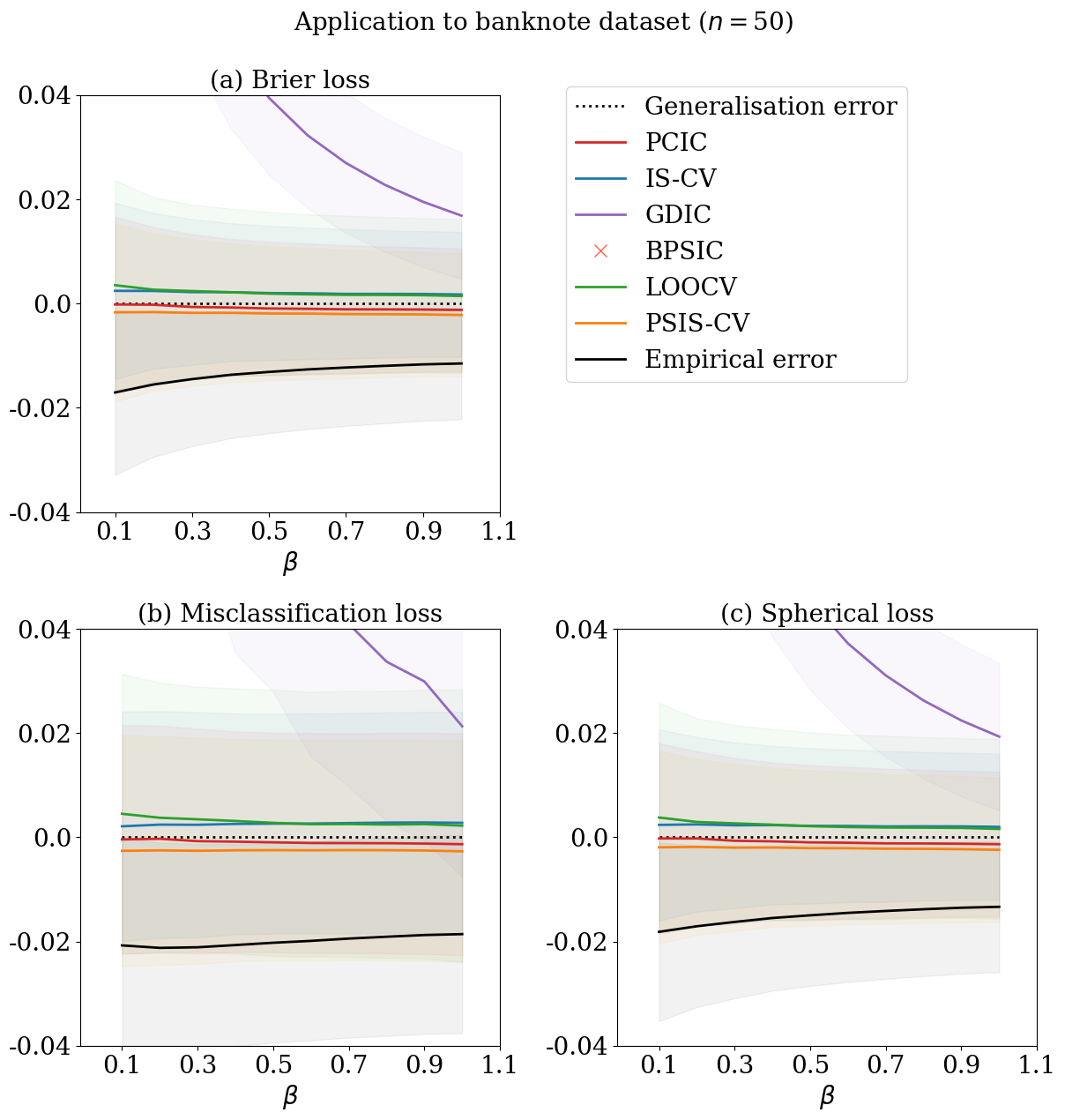
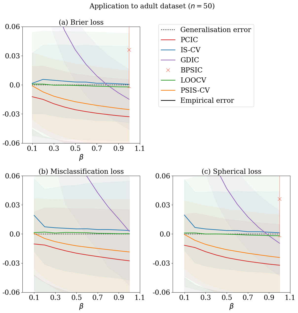
Here, we demonstrate the application of to understanding the predictive behaviour of OPS estimators with different values of . We use two sets of classification data from UCI Machine Learning Repository (Dua and Graff, 2017), namely, the banknote authentication data set and the adult data set. The banknote authentication data set classifies genuine and forged banknote-like specimens based on four image features. The adult data set predicts whether income exceeds K/yr based on 14 features from census data. We work with the generalised posterior distribution based on the logistic regression
where is the sigmoid function: . We consider predictive evaluation of OPS estimators using three major classification losses, the Brier loss, the misclassification loss, and the spherical loss:
where for the observation, is given by using . The misclassification loss is non-differentiable with respect to and our theoretical results may not imply accurate generalisation error estimation; so, we confirm the applicability by numerical experiments. First, we randomly split the whole data into a training dataset of a sample size 50, 20 times. The test dataset is set to be the remaining. We then calculate the empirical errors using the training dataset, and the average of generalisation errors using the test dataset. We used 3980 MCMC samples after thinning out by 5 and a burnin period of length 100. The MCMC algorithm here employs the Gibbs sampler based on Polya-Gamma augmentation (Polson et al., 2013).
Figures 1 and 2 display the average values of generalisation error estimates relative to the average of the generalisation errors. The exact LOOCV is very close to the average of the generalisation error irrelevant to the loss and the dataset, but its computational cost is almost prohibitive. GDIC is not close to the average of the generalisation error. BPSIC works only for and a differentiable evaluation function. The proposed method successfully estimates the generalisation errors of OPS estimators for all three evaluation functions, including the non-differentiable evaluation function. IS-CV and PSIS-CV are comparable to the proposed method; therefore, we cannot reach a conclusion regarding the performance difference of this setting.
3.2 Application to Bayesian hierarchical models
We then apply the proposed methods to predictive evaluation of Bayesian hierarchical modeling. Here we shall work with a simple two-level normal model:
where s are assumed to be given, is the sample size of the -th group (), and is the number of groups. Here we assume that is equal to 1 and denote by , which is always possible by the sufficiency reduction. The prior distributions of and are specified by the scale mixture of the normal distribution with the half Cauchy distribution and by the half normal distribution, respectively:
where and are hyper parameters.
We measure the prediction accuracy of the information fusion in the Bayesian hierarchical structure across groups by (unscaled) loss
The working posterior in this application is rewritten as
where is the normal density with mean and variance . So, becomes
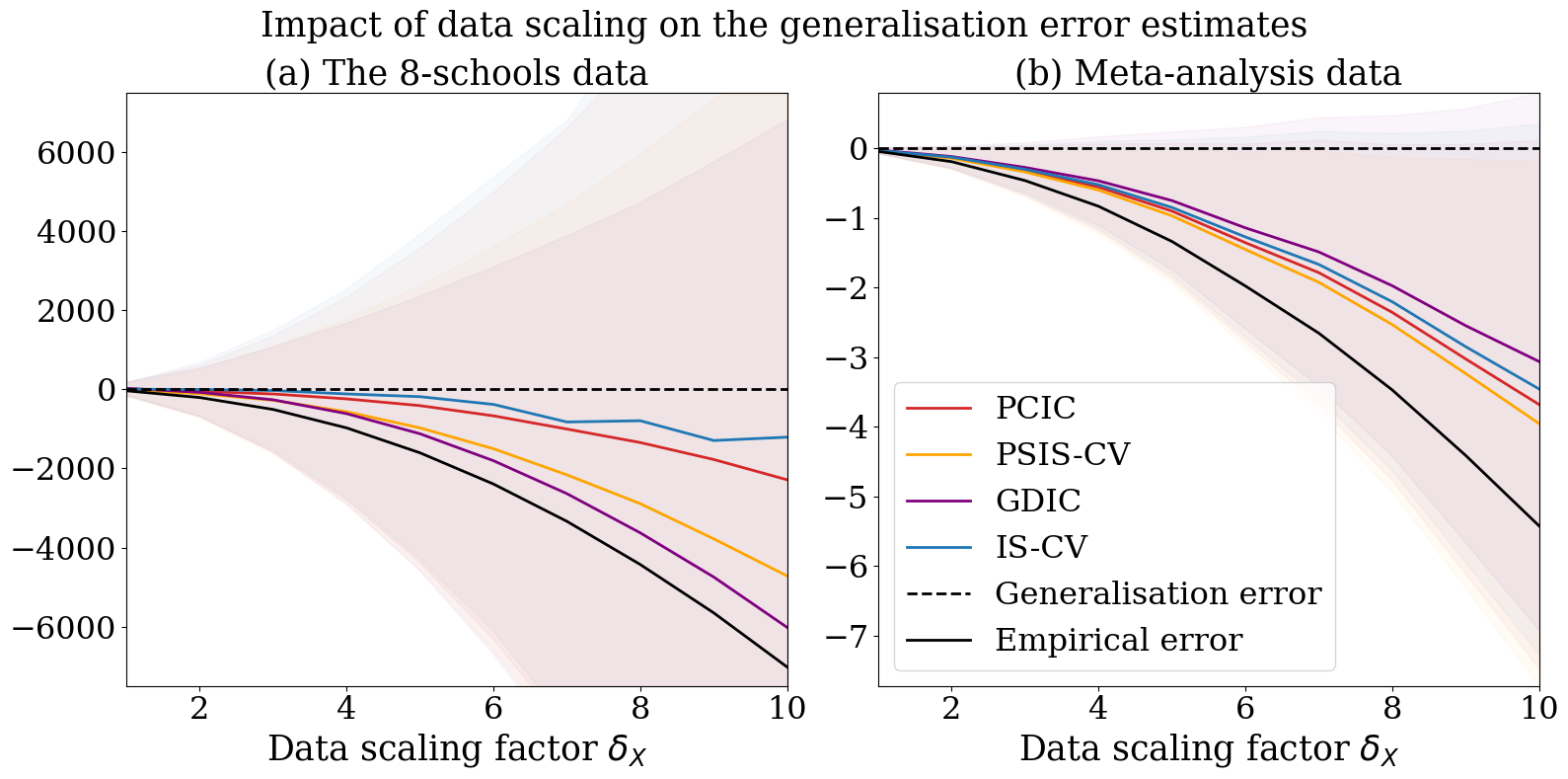
To check the behaviour, we use two datasets commonly used in the demonstration of the Bayesian hierarchical modeling. One is the 8-schools data: the dataset consists of coaching effects with the standard deviations in different high schools in New Jersey; see Table 5.2 of Gelman et al. (2013). The other is the meta-analysis data from Yusuf et al. (1985): the dataset consists of clinical trials of -blockers for reducing mortality after myocardial infarction; see Table 5.4 of Gelman et al. (2013). We apply empirical log-odds transformation so as to employ the normal model described above as in Section 5.8 of Gelman et al. (2013).
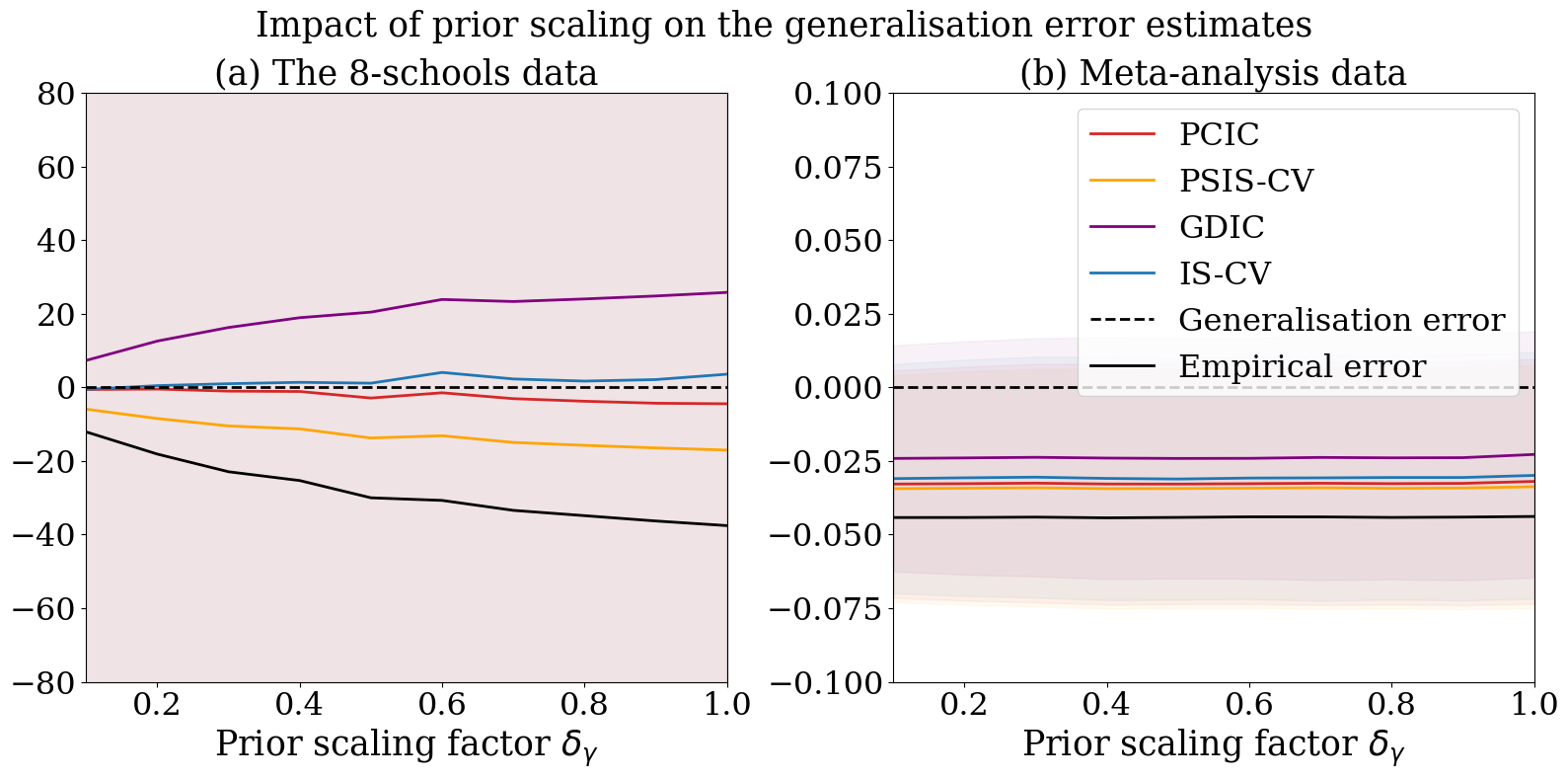
We design two types of experiments. One is changing the data scale by multiplying the data scaling factor to s. The other is changing the prior scale by multiplying the prior scaling factor to . We fix and set as initial values. In the experiments, we first randomly split the original datasets of groups into the training data of the remaining groups and the test data of groups 20 times. We then obtain 5000 posterior samples using PyMC (Abril-Pla et al., 2023), calculate the empirical errors and the generalisation error estimates using the training data set, and calculate the average of generalisation errors using the test data set.
Figure 3 displays the generalisation error estimates relative to the average generalisation errors along with the change of the data scaling factor . Figure 4 displays those along with the change of the prior scaling factor . As the data scaling factor becomes largers, all esitmates deteriorate (becomes far from the generalisation error) but the deteriorating rates of IS-CV and PCIC are slower than that of PSIS-CV. Fro any prior scaling factor, IS-CV and PCIC are closer to the generalisation error than PSIS-CV. GDIC is a relatively good metric for the meta-analysis data but not for the 8-school data.
3.3 Application to Bayesian regression in the presence of influential observations
We next apply the proposed method to Bayesian regression the presence of influential observations. The presence of influential observations impacts the variability of the case-deletion importance sampling weights, as discussed in Peruggia (1997), which results in the instability of IS-CV.
Here, we focus on the performance comparison between our method and IS-CV in Bayesian regression with influential observations. We work with the following Bayesian regression model in Peruggia (1997): Let be the sample size and let () be the covariates. Then,
| (13) |
where denotes the inverse gamma distribution, denotes the inverse Wishart distribution, and denotes the identity matrix. Three quantities are hyperparameters, and we fix . The score function in this subsection is simply the log-likelihood. For the loss functions, we use , , scaled and scaled losses:
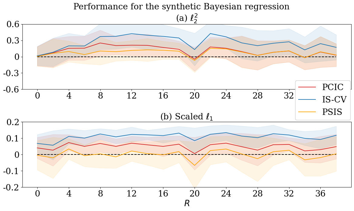
We begin with the following synthetic Bayesian regression model: for a given , are fixed to
and then are given as
where s are i.i.d. from the standard Gaussian distribution, and , , and are unknown parameters. We assign (0,1,1) to the true values of . We set 50 to the sample size . For each , we simulate the training data set 50 times and obtain 50 values of , PSIS-CV, and IS-CV. We then calculate the average of the generalisation errors using a test data set with a sample size of 10. By using the same Gibbs sampler as in Peruggia (1997), we obtained 2000 MCMC samples after thinning out by 10 and a burnin period of length 10000.
Figure 5 displays the comparison between and IS-CV. Consider . For , the performance of the two methods does not differ. For , the bias of IS-CV relative to the average of the generalisation errors, is larger than that of . Consider . In this case, for all , the bias of IS-CV, relative to the average of the generalisation errors, is larger than those of and PSIS-CV. In particular, PSIS-CV performs the best for this loss.
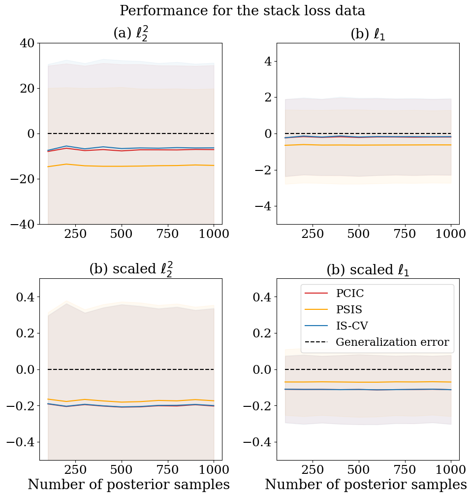
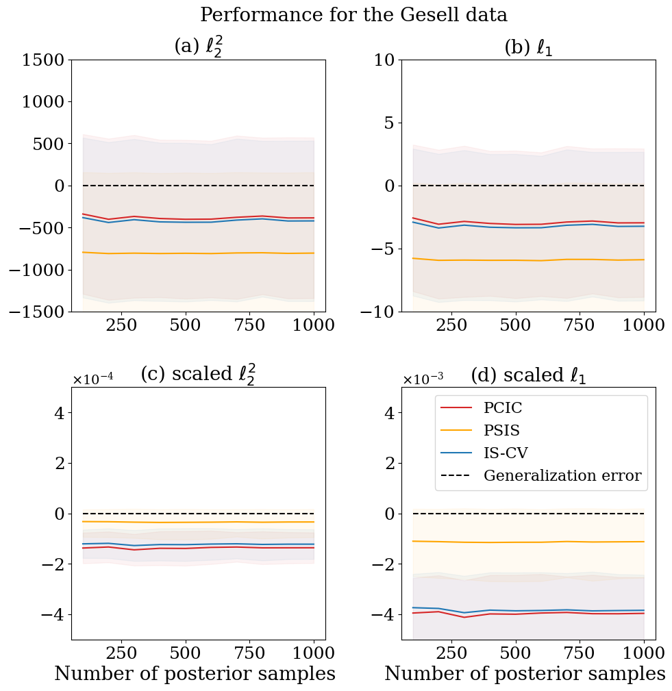
We next employ two real datasets containing influential observations. One is the the stack loss data: The data consists of days of measurements with three condition records . The other is the Gesell data: This consists of children’s records of the age at which they first spoke and their Gesell Adaptive Score . These datasets are known to contain influential observations; the indices for influential observations are and , respectively. In the experiments, we first randomly split the original datasets into the training data of samples and the test data of samples 20 times. We then obtain posterior samples with different sample sizes, calculate the empirical errors and the generalisation error estimates using the training data set, and calculate the average of generalisation errors using the test data set.
Figures D.1 and D.2 display the results. Overall, and IS-CV works better than PSIS-CV for the unscaled losses ( and losses), whereas PSIS-CV works the best for the scaled losses. One of the reasons is that the scaled losses works similar (in fact, the scaled loss is the half of log likelihood), and the weight smoothing in PSIS-CV only depends only on log-likelihood.
3.4 Application to eliminating biases due to strong priors
When using strong priors, WAIC is shown to have a bias in the generalisation error estimation (e.g., Vehtari et al. (2017); Ninomiya (2021)). We here employ to eliminate this bias. We begin with focusing on a simple example that enables a full analytic calculus and then provide a general scheme applicable to general models.
Analytic calculus in a location-shift model: Consider a simple location-shift model, where the observations follow
Here, is a vector in , and the error terms are i.i.d. from a possibly non-Gaussian distribution with mean zero and covariance matrix identity matrix. Consider the generalised posterior distribution given by
where is the norm in ; then, the generalised posterior distribution is with
and the score function in this case is , where let and let be the identity matrix.
Consider the evaluation function with a symmetric positive definite matrix . Thus, the Gibbs generalisation gap is given by
| (14) |
while the posterior covariance is given by
| (15) |
where and the detailed calculi are given in Appendix C. Thus, we obtain
| (16) |
where we let
From (16), we conclude that in simple location-shift models, under the assumption
| (17) |
even the naive estimates well the Gibbs generalisation error regardless of the dimension and the distribution of the error term. For non-strong priors (), we can make the assumption in (17). For strong priors (), we cannot expect the validity of the assumption, and the bias term
remains. Our generalised Bayesian framework provides a simple modification to remove this bias. Add the log-prior density (up to constant) divided by to ;
Then, we have
| (18) |
with an -term that is independent of , which implies that the bias term in the naive can be removed by changing the naive average posterior covariance to
A scheme for general models: The above scheme is applicable in eliminating the bias of in general models by changing the average posterior variance to
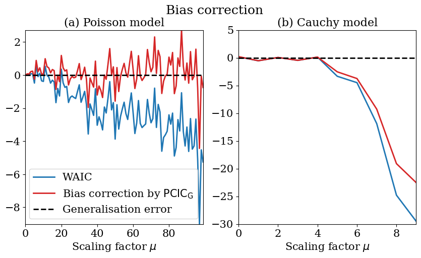
We check the effectiveness of this scheme by using the Poisson model and the Cauchy model. Figure 6 demonstrates the results for the Poisson model with the conjugate Gamma prior and the multivariate Cauchy model with the Cauchy prior; that is, the observation and the prior in the Poisson model are described as
while those in the Cauchy model are described as
After setting and , we vary the scaling factor . In the Poisson conjugate model, the bias correction successfully works as depicted in Figure 6 (a). In the Cauchy model, the bias correction does work but there appears an additional non-negligible bias. Note that such bias also appears with large data scaling in the application to Bayesian hierarchical models; see Figure 3.
4 Discussions
In this section, we discuss the following three topics:
-
•
the applicability in high dimensions;
-
•
the application to defining a case-influence measure; and
-
•
possibility of different definitions of generalisation errors.
4.1 Applicability in high dimensions
We first check the applicability of our methodologies as well as IS-CV and PSIS-CV in high dimensional models. If we view the location-shift model in Subsection 3.4 from a different perspective, the arguments in that subsection suggest that PCIC can be applied even in high-dimensional settings. This does not contradict the results of Okuno and Yano (2023), where WAIC is shown to work even in overparameterised linear regression models. However, since these fully rely on the model’s structures, further experiments are required.
Here, we employ the Poisson sequence model, a canonical model for count-data analysis. Incorporating the high-dimensional structure with Poisson sequence model becomes important in recent count-data analysis (Komaki, 2006; Datta and Dunson, 2016; Yano et al., 2021; Hamura et al., 2022; Paul and Chakrabarti, 2024). The working model here is
where is an index for the observation, is an index for the coordinate, and denotes the product of measures. In this model, each observation given follows from the -dimensional independent Poisson distribution. For example, in spatio-temporal count-data analysis, may be the index for the year and may be the index for the observation site such as a district; see Datta and Dunson (2016); Yano et al. (2021); Hamura et al. (2022) for the details.
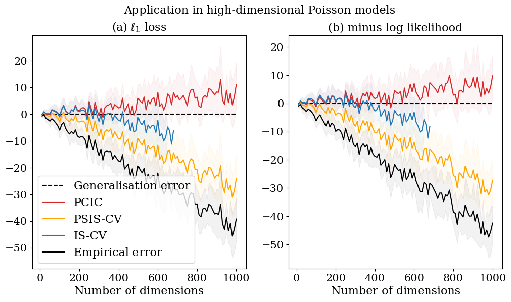
We start with checking the behaviours of generalisation error estimates along with the change of the number of dimensions. We fix the sample size to 10. In this numerical experiment, we work with the Stein-type shrinkage prior proposed by Komaki (2006):
where and . The reason of this prior choice is that it is non-informative, efficiently combines information across coordinates, and has an efficient exact sampling algorithm. We set and . For the true values of s, we set
Figure 7 depicts the success of even in high-dimensional models, though we have not ensured it theoretically. Okuno and Yano (2023) shows the success of even in overparameterized linear regression models; Giordano and Broderick (2023) discusses the Bayesian infinitesimal jackknife approximation of the variance in high dimensions. These together with our result might deliver a new research direction focusing on understanding the behaviour of the posterior covariance in high-dimensions. Understanding this might require further theoretical investigations on the approximation of cross validation in high dimensions (e.g., Rad and Maleki, 2020) and Bayesian central limit theorem in high-dimensions (e.g., Panov and Spokoiny, 2015; Yano and Kato, 2020; Kasprzaki et al., 2023).
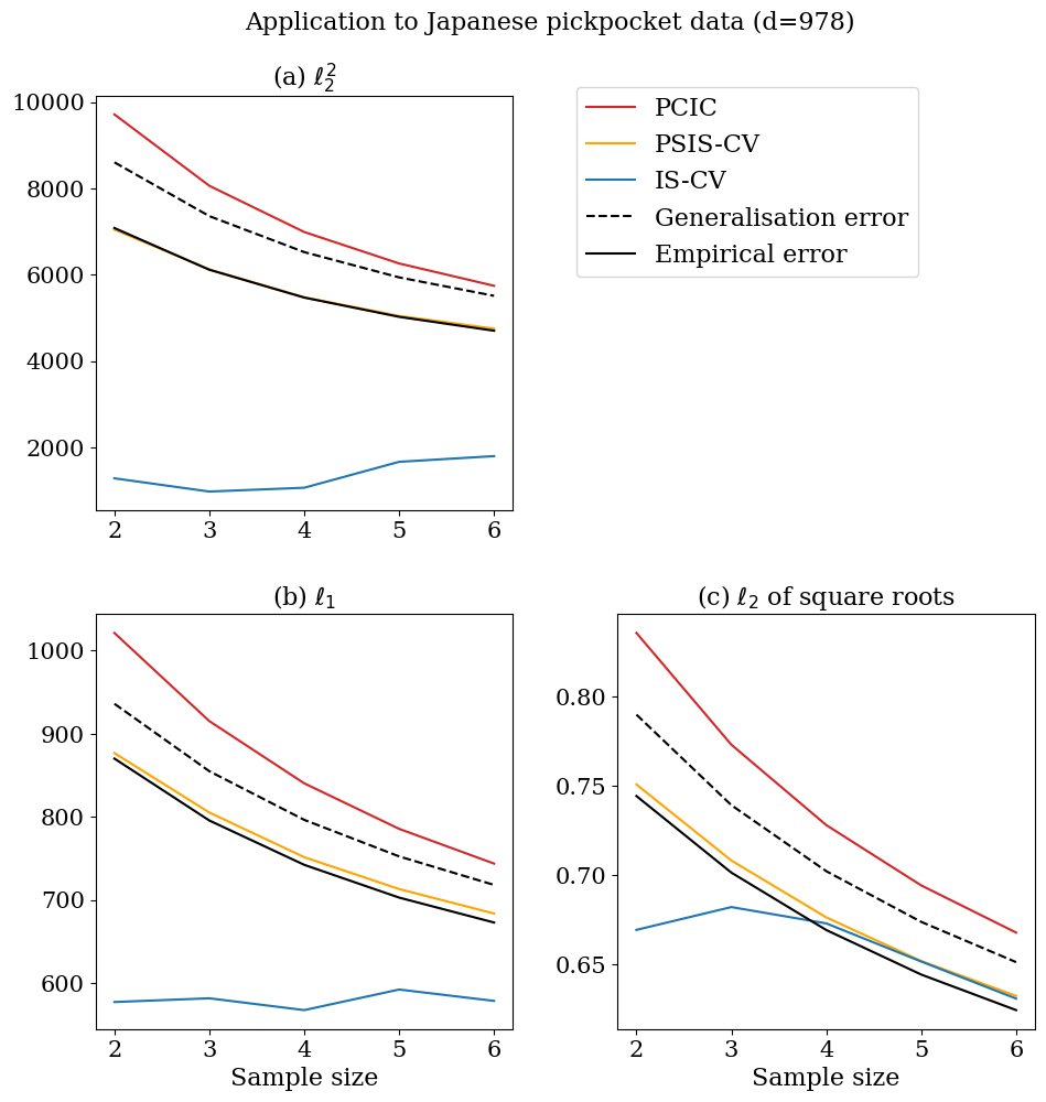
We next check the behaviours in the application to real data. We employ Japanese pickpocket data from Tokyo Metropolitan Police Department (2025). This data reports the total numbers of pickpockets in each year in Tokyo Prefecture, and are classified by town and also by the type of crimes. We use pickpocket data from 2012 to 2018 at 978 towns in 8 wards; So, we work with the Poisson sequence model (, ; is the number of years we use in the analysis). For , we consider all combinations of selecting out of years, and use each combination as training data while treating the remaining items as test data. For each training and test pair, we calculate the generalisation error as well as its estimates (, PSIS-CV, IS-CV, and the empirical error), and take their averages.
Figure 8 displays the results for three loss functions: loss, loss, and
For all loss functions, estimates the generalisation error well.
4.2 Application to defining a case-influence measure
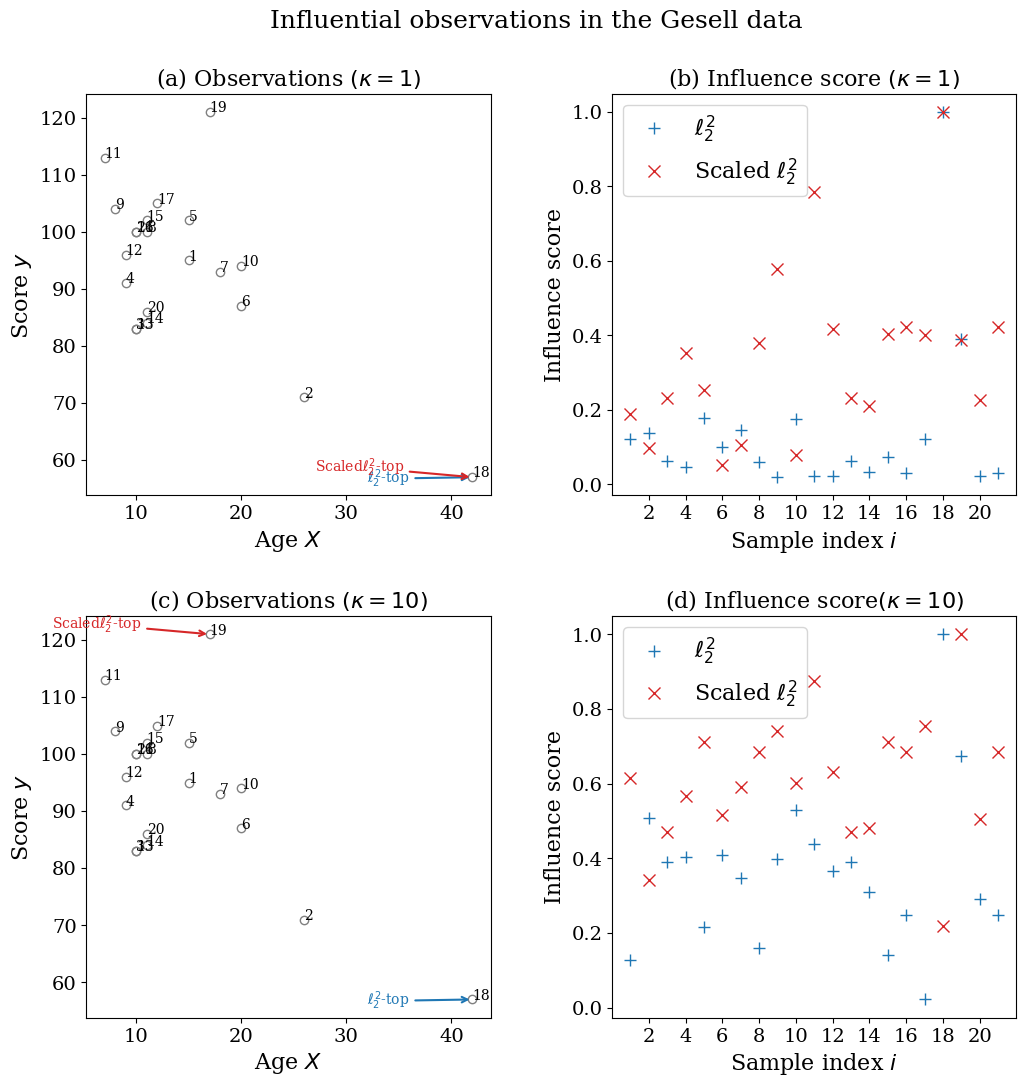
We next consider an application of the proposed method to defining yet another case-influence measure. From the perspective of estimating the generalisation error, the posterior covariance
expresses the contribution of each observation in filling the generalisation gap. So, we can utilise it to define yet another Bayesian case-influence measure in prediction. When and , this coincides with the Bayesian local case sensitivity defined in Millar and Stewart (2007); Thomas et al. (2018). Note that this is not always positive except for ; so we standardize it and take the absolute value.
Figure 9 showcases how the measure works in the Gesell data discussed in Subsection 3.3, where we use the unscaled and the scaled losses, and the score function is log likelihood. For relatively light-tailed prior (), the top-1 influential observations are the same for both losses (Figure 9 a) . For relatively heavy-tailed prior (), the top-1 influential observations are different (Figure 9 c).
Here we compare our results with those in Millar and Stewart (2007), where two types of sensitivities (parameter-scale and observation-scale) are defined. First, our results with the unscaled loss are similar to the results with the observation-scale sensitivity in Millar and Stewart (2007), and the results with the scaled loss are similar to the results with the parameter-scale sensitivity in Millar and Stewart (2007); Second, our results with the relatively light-tailed prior are similar to Millar and Stewart (2007)’s results in the known-variance case, and our results with the relatively heavy-tailed prior are similar to Millar and Stewart (2007)’s results the unknown-variance case with Bernard’s reference prior. Our result as well as Millar and Stewart (2007) and Thomas et al. (2018) suggest that the case influences also vary depending on the choice of loss functions. Also, our result as well as Millar and Stewart (2007) suggest that the case influences vary depending on the prior specification.
4.3 Possibility of different definitions of generalisation errors
Although we only consider the Gibbs and plug-in generalization errors, following the literature (e.g., Ando, 2007; Underhill and Smith, 2016), one could alternatively define the generalization error as
where is a scoring rule (Gneiting and Raftery, 2007; Dawid et al., 2016), and is a parametric model. This may be viewed as a natural extension of the generalization error used in WAIC (Watanabe, 2010b).
In the binary prediction setting discussed in Subsection 3.1, the plug-in generalization errors coincide with this definition. However, our current methodologies do not accommodate this scoring-rule-based generalisation error in more general prediction scenarios. In this paper, we have not pursued this direction because it remains unclear whether the use of the Bayesian predictive density is theoretically justified. While for the log score, the Bayesian predictive density is the Bayes solution (Aitchison, 1975), it is not necessarily the Bayes solution for other loss functions (see, e.g., Corcuera and Giummolè, 1999).
Recently, a quasi-Bayesian framework associated with scoring rules has been developed (Giummolè et al., 2019; Matsubara et al., 2024). Thus, extending our understanding of scoring-rule-based generalization errors in conjunction with such quasi-Bayesian theory would be an important future research direction.
5 Conclusion
We have proposed a novel, computationally low-cost method of estimating the Gibbs generalisation errors and plugin generalisation errors for arbitrary loss functions. We have demonstrated the usefulness of the proposed method in privacy-preserving learning, Bayesian hierarchical modeling, Bayesian regression modeling in the presence of the influential observations, and discussed the applicability in high dimensional statistical models.
Our numerical experiments suggest that IS-CV, PSIS-CV, and PCIC are useful tools for assessing generalisation errors. However, when applied to high-dimensional models (Subsection 4.1) or when the magnitude of the data is large (Subsection 3.2), PCIC remains effective even under such settings. Detailed theoretical analyses remain an important direction for future research.
An important practical implication of this study is that the posterior covariance provides an easy-to-implement generalisation error estimate for arbitrary loss functions, and can avoid the cumbersome refitting in LOOCV as well as the importance sampling technique that is sensitive to the presence of influential observations. Also, theoretical connections between WAIC, the Bayesian sensitivity analysis, and the infinitesimal jackknife approximation of Bayesian LOOCV are clarified. by our proof for the asymptotic unbiasedness .
Acknowledgement
The authors would like to thank the handling editor, the associate editor, and two anonymous referees for their comments that have improved the quality of the paper. Also, the authors would like to thank Akifumi Okuno, Hironori Fujisawa, Yoshiyuki Ninomiya, and Yusaku Ohkubo for providing them with fruitful discussions.
Funding
This work was supported by Japan Society for the Promotion of Science (JSPS) [Grant Nos. 19K20222, 21H05205, 21K12067], the Japan Science and Technology Agency’s Core Research for Evolutional Science and Technology (JST CREST) [Grant No. JPMJCR1763], and the MEXT Project for Seismology toward Research Innovation with Data of Earthquake (STAR-E) [Grant No. JPJ010217].
Code availability statements
The python code is available at https://github.com/kyanostat/PCIC4GL.
References
- Abadi et al. (2016) Abadi, M., Chu, A., Goodfellow, I., McMahan, H. B., Mironov, I., Talwar, K. and Zhang, L. (2016) Deep learning with differential privacy. Proceedings of the 2016 ACM SIGSAC Conference on Computer and Communications Security, 308–318.
- Abril-Pla et al. (2023) Abril-Pla, O., Andreani, V., Carroll, C., Dong, L., Fonnesbeck, C. J., Kochurov, M., Kumar, R., Lao, J., Luhmann, C. C., Martin, O. A. et al. (2023) Pymc: a modern, and comprehensive probabilistic programming framework in python. PeerJ Computer Science, 9, e1516.
- Aitchison (1975) Aitchison, J. (1975) Goodness of prediction fit. Biometrika, 62, 547–554.
- Akaike (1973) Akaike, H. (1973) Information theory and an extension of the maximum likelihood principle. In Proceedings of the 2nd Intertnational Symposium on Information Theory (eds. B. Petrov and F. Csáki), 267–281.
- Ando (2007) Ando, T. (2007) Bayesian predictive information criterion for the evaluation of hierarchical Bayesian and empirical Bayes models. Biometrika, 94, 443–458.
- Beirami et al. (2017) Beirami, A., Razaviyayn, M., Shahrampour, S. and Tartokh, V. (2017) On optimal generalizability in parametric learning. In Advances in Neural Information Processing Systems, 3458–3468.
- Bissiri et al. (2016) Bissiri, P., Holmes, C. and Walker, S. (2016) A general framework for updating brief distributions. Journal of the Royal Statistical Society: Series B (Statistical Methodology), 78, 1103–1130.
- Chernozhukov and Hong (2003) Chernozhukov, V. and Hong, H. (2003) An MCMC approach to classical estimation. Journal of Econometrics, 115, 293–346.
- Corcuera and Giummolè (1999) Corcuera, J. and Giummolè, F. (1999) A generalized Bayes rule for prediction. Scandinavian Journal of Statistics, 26, 265–279.
- Datta and Dunson (2016) Datta, J. and Dunson, D. (2016) Bayesian inference on quasi-sparse count data. Biometrika, 103, 971–983.
- Dawid et al. (2016) Dawid, A., Musio, M. and Ventura, L. (2016) Minimum scoring rule inference. Scandinavian Journal of Statistics, 43, 123–138.
- Desfontaines and Pejó (2020) Desfontaines, D. and Pejó, B. (2020) Sok: Differential privacies. Proceedings on Privacy Enhancing Technologies, 2, 288–313.
- Dua and Graff (2017) Dua, D. and Graff, C. (2017) UCI machine learning repository. URL: http://archive.ics.uci.edu/ml.
- Dwork (2006) Dwork, C. (2006) Differential privacy. In Proceedings of the 33rd International conference on Automata, Languages and Programming, Part II, 1–12.
- Geisser (1975) Geisser, S. (1975) The predictive sample reuse method with applications. Journal of American Statistical Association, 70, 320–328.
- Gelfand et al. (1992) Gelfand, A., Dey, D. and Chang, H. (1992) Model determination using predictive distributions with implementation via sampling-based methods. In Bayesian Statistics (eds. J. Bernardo, J. Berger, A. Dawid and A. Smith), 147–167. Oxford University Press.
- Gelman et al. (2013) Gelman, A., Carlin, J., Stern, H., Dunson, D., Vehtari, A. and Rubin, D. (2013) Bayesian Data Analysis, 3rd Edition. Chapman and Hall/CRC.
- Giordano and Broderick (2023) Giordano, R. and Broderick, T. (2023) The Bayesian infinitesimal jackknife for variance. ArXiv:2305.06466.
- Giordano et al. (2018) Giordano, R., Broderick, T. and Jordan, M. (2018) Covariances, robustness, and variational Bayes. Journal of Machine Learning Research, 19, 1–49. URL: http://jmlr.org/papers/v19/17-670.html.
- Giordano et al. (2019) Giordano, R., Stephenson, W., Liu, R., Jornan, M. and Broderick, T. (2019) A Swiss army infinitesimal jackknife. Proceedings of the 22nd International Conference on Artificial Intelligence and Statistics (AISTATS) 2019, 89.
- Giummolè et al. (2019) Giummolè, F., Mameli, V., Ruli, E. and Ventura, L. (2019) Objective Bayesian inference with proper scoring rules. Test, 28, 728––755.
- Gneiting and Raftery (2007) Gneiting, T. and Raftery, A. (2007) Strictly proper scoring rules, prediction, and estimation. Journal of the American Statistical Association, 102, 359–378.
- Hamura et al. (2022) Hamura, H., Irie, K. and Sugasawa, S. (2022) On global-local shrinkage priors for count data. Bayesian Analysis, 17, 545–564.
- Iba (2023) Iba, Y. (2023) W-kernel and essential subspace for frequencist’s evaluation of Bayesian estimators. ArXiv:2311.13017.
- Iba and Yano (2023) Iba, Y. and Yano, K. (2023) Posterior covariance information criterion for weighted inference. Neural computation, 35, 1–22.
- Jewson et al. (2023) Jewson, J., Ghalebikesabi, S. and Holmes, C. (2023) Differentially private statistical inference through -divergence one posterior sampling. Proceedings of 37th Conference on Neural Information Processing Systems (NeurIPS 2023).
- Jiang and Tanner (2008) Jiang, W. and Tanner, M. (2008) Gibbs posterior for variable selection in high-dimensional classification and data mining. The Annals of Statistics, 36, 2207–2231.
- Kasprzaki et al. (2023) Kasprzaki, M., Giordano, R. and Broderick, T. (2023) How good is your Laplace approximation of the Bayesian posterior? finite-sample computable error bounds for a variety of useful divergences. ArXiv:2209.14992.
- Koh and Liang (2017) Koh, P. and Liang, P. (2017) Understanding black-box predictions via influence functions. In Proceedings of the 34th International Conference on Machine Learning, 1885–1894.
- Komaki (2006) Komaki, F. (2006) A class of proper priors for Bayesian simultaneous prediction of independent Poisson observables. Journal of Multivariate Analysis, 97, 1815–1828.
- Konishi and Kitagawa (1996) Konishi, S. and Kitagawa, G. (1996) Generalised information criteria in model selection. Biometrika, 83, 875–890.
- Mastubara et al. (2022) Mastubara, T., Knoblauch, J., Briol, F. and Oates, C. (2022) Robust generalised Bayesian inference for intractable likelihoods. Journal of the Royal Statistical Society: Series B (Statistical Methodology), 84, 997–1022.
- Matsubara et al. (2024) Matsubara, T., Knoblauch, J., Briol, F.-X. and Oates, C. (2024) Generalized bayesian inference for discrete intractable likelihood. Journal of the American Statistical Association, 119, 2345–2355.
- Millar and Stewart (2007) Millar, R. and Stewart, W. (2007) Assessment of locally influential observations in Bayesian models. Bayesian Analysis, 2, 365–384.
- Miller and Dunson (2019) Miller, J. and Dunson, D. (2019) Robust Bayesian inference via coarsening. Journal of the American Statistical Association, 114, 1113––1125.
- Minami et al. (2016) Minami, K., Arai, H., Sato, I. and Nakagawa, H. (2016) Differential privacy without sensitivity. In Advances in Neural Information Processing Systems (eds. D. Lee, M. Sugiyama, U. Luxburg, I. Guyon and R. Garnett), vol. 29.
- Mironov (2017) Mironov, I. (2017) Rènyi differential privacy. 2017 IEEE 30th Computer Security Foundations Symposium (CSF), 263–275.
- Nakagawa and Hashimoto (2020) Nakagawa, T. and Hashimoto, S. (2020) Robust Bayesian inference via -divergence. Communications in Statistics - Theory and Methods, 49, 343–360.
- Ninomiya (2021) Ninomiya, Y. (2021) Prior intensified information criterion. ArXiv: 2110.12145.
- Okuno and Yano (2023) Okuno, A. and Yano, K. (2023) A generalization gap estimation for overparameterized models via the Langevin functional variance. Journal of Computational and Graphical Statistics, 32, 1287–1295.
- Panov and Spokoiny (2015) Panov, M. and Spokoiny, V. (2015) Finite sample Bernstein–von Mises theorem for semiparametric problems. Bayesian Analysis, 10, 665–710.
- Paul and Chakrabarti (2024) Paul, S. and Chakrabarti, A. (2024) Asymptotic bayes optiamlity for sparse count data. URL: https://arxiv.org/abs/2401.05693.
- Pérez et al. (2006) Pérez, C., Martin, J. and Rufo, M. (2006) MCMC-based local parametric sensitivity estimations. Computational Statistics & Data Analysis, 51, 823–835.
- Peruggia (1997) Peruggia, M. (1997) On the variability of case-deletion importance sampling weights in the Bayesian linear model. Journal of the Ametican Statistical Association, 92.
- Polson et al. (2013) Polson, N., Scott, J. and Windle, J. (2013) Bayesian inference for logistic models using Pólya–Gamma latent variables. Journal of the American Statistical Association, 108, 1339–1349.
- Rad and Maleki (2020) Rad, K. and Maleki, A. (2020) A scalable estimate of the extra-sample prediction error via approximate leave-one-out. Journal of Royal Statistical Society: Series B, 82, 965–996.
- Ribatet et al. (2012) Ribatet, M., Cooley, D. and Davison, A. (2012) Bayesian inference from composite likelihoods, with an application to spatial extremes. Statistica Sinica, 22, 813–845.
- Shibata (1989) Shibata, R. (1989) Statistical aspects of model selection, 215–240. Springer-Verlag.
- Silva and Zanella (2023) Silva, L. and Zanella, G. (2023) Robust leave-one-out cross-validation for high-dimensional Bayesian models. Journal of the American Statistical Association. In press.
- Spiegelhalter et al. (2002) Spiegelhalter, D., Best, N., Carlin, B. and van der Linde, A. (2002) Bayesian measures of model complexity and fit. Journal of the Royal Statistical Society: Series B, 64, 583–639.
- Stone (1974) Stone, M. (1974) Cross-validatory choice and assessment of statistical predictions (with discussion). Journal of the Royal Statistical Society: Series B, 36, 111–147.
- Takeuchi (1976) Takeuchi, K. (1976) Distribution of informational statistics and a criterion of model fitting (in japanese). Suri-Kagaku (Mathematic Sciences), 153, 12–18.
- Thomas et al. (2018) Thomas, Z., MacEachern, S. and Peruggia, M. (2018) Reconciling curvature and importance sampling based procedures for summarizing case influence in Bayesian models. Journal of the American Statistical Association, 113, 1669–1683.
- Tokyo Metropolitan Police Department (2025) Tokyo Metropolitan Police Department (2025) The number of crimes in tokyo prefecture by town and type. Https://www.keishicho.metro.tokyo.lg.jp/about_mpd/jokyo_tokei/jokyo/.
- Underhill and Smith (2016) Underhill, N. and Smith, J. (2016) Context-dependent score based Bayesian information criteria. Bayesian Analysis, 11, 1005–1033.
- Vehtari (2002) Vehtari, A. (2002) Discussion of“Bayesian measures of model complexity and fit” by spiegelhalter et al. Journal of Royal Statistical Society B, 64, 620.
- Vehtari et al. (2017) Vehtari, A., Gelman, A. and Gabry, J. (2017) Practical Bayesian model evaluation using leave-one-out cross-validation and WAIC. Statistics and Computing.
- Vehtari and Lampinen (2003) Vehtari, A. and Lampinen, J. (2003) Expected utility estimation via cross-validation. In Bayesian statistics (eds. J. Bernardo, M. Bayarri, J. Berger, A. Dawid, D. Heckerman, A. Smith and M. West). Oxford University Press.
- Vehtari and Ojanen (2012) Vehtari, A. and Ojanen, J. (2012) A survey of Bayesian predictive methods for model assessment, selection and comparison. Statistics Surveys, 6, 142––228.
- Vehtari et al. (2024) Vehtari, A., Simpson, D., Gelman, A., Yao, Y. and Gabry, J. (2024) Pareto smoothed importance sampling. Journal of Machine Learning Research, 25, 1–58.
- Wang et al. (2015a) Wang, Y.-X., Fienberg, S. and Smola, A. (2015a) Privacy for free: Posterior sampling and stochastic gradient Monte Carlo. In Proceedings of the 32nd International Conference on Machine Learning, vol. 37, 2493–2502.
- Wang et al. (2015b) — (2015b) Privacy for free: Posterior sampling and stochastic gradient Monte Carlo. Proceeding of the 32nd International Conference on Machine Learning (ICML’15), 2493–2502.
- Watanabe (2010a) Watanabe, S. (2010a) Asymptotic equivalence of Bayes cross validation and widely applicable information criterion in singular learning theory. Journal of Machine Learning Research, 11, 3571–3594.
- Watanabe (2010b) — (2010b) Equations of states in singular statistical estimation. Neural Networks, 23, 20–34.
- Watanabe (2018) — (2018) Mathematical Theory of Bayesian Statistics. Chapman & Hall/CRC.
- Yano et al. (2021) Yano, K., Kaneko, R. and Komaki, F. (2021) Minimax predictive density for sparse count data. Bernoulli, 27, 1212–1238.
- Yano and Kato (2020) Yano, K. and Kato, K. (2020) On frequentist coverage errors of Bayesian credible sets in moderately high dimensions. Bernoulli, 26, 616–641.
- Yusuf et al. (1985) Yusuf, S., Pero, R., Lewis, J., Collins, R. and Sleight, P. (1985) Beta blockade during and after myocardial infarction: an overview of the randomized trials. Progress in Cardiovascular Diseases, 27, 335–371.
Appendix A Conditions for the theorem
The conditions in this paper are as follows: In the conditions, is redefined by subtracting from the original .
-
(C1)
The difference is of the order ;
-
(C2)
The following relation holds:
-
(C3)
There exists an integrable function such that for all ,
Remark A.1 (Discussion on the conditions).
First, consider Condition C1. In regular statistical models and smooth evaluation functions, the result of Underhill and Smith (2016) implies that the order of is . that the expected generalisation error subtracted by its minimum with respect to the parameter
is of order . We briefly discuss on it. Let be the minimizer of . The Taylor expansion yields
Thus, we get
The order of the term is controlled by the difference between the posterior mean and ; so it is of order . The order of the term is determined by Lemma 3 of Underhill and Smith (2016); so it is of order , which concludes the order of the expected (subtracted) generalisation error. For singular statistical models and log-likelihoods, the result of Watanabe (2010b) implies that the order of (subtracted by its minimum) is . Thus, Condition C1 usually holds.
Condition C2 is a condition for the residual. For regular statistical models and smooth evaluation functions, the Taylor expansion implies that the order of the left hand side is and less than the order of . For singular statistical models and log-likelihoods, we refer to Watanabe (2018). Finally, Condition C3 is a mild condition for assuming the existence of expectation.
Appendix B Proof for Lemma 2.3
This appendix provides the proof of Lemma 2.3.
The Lebesgue dominated convergence theorem ensures the exchange of differentiation and integration in under Condition C3. Then, considering
gives
which implies
Further, we have
and
which implies
and completes the proof. ∎
Appendix C Detailed calculations used in Section 3.4
This appendix provides the detailed calculation used in Section 3.4. The calculation employs the following lemma.
Lemma C.1 (Kumar, 1973).
Let be a random vector from . For symmetric matrices and , we have
Step 1. Establishing (15): Let us begin by expanding . For , we have
where and . Lemma C.1 gives
and thus we get
| (C.1) |
Further, for , we have
| (C.2) |
Combining (C.1) and (C.2) yields
which implies (15).
Step 2. Establishing (16): Next, we take the expectation of . Let . Then, we have
which implies (16).
Step 3. Establishing (18): Finally, we consider . For , we have
and we have
Combining these yields
This, together with the identity
yields (18).
References for this appendix
-
[1]
Kumar, A. (1973) Expectation of products of quadratic forms. Sankha, 35, 359–362.
Appendix D Additional figures
This appendix provides additional figures. Figure D.1 depicts the result for the stack loss data; see Subsection 3.2 for details. Figure D.2 depicts the result for the Gesell data; see Subsection 3.2 for details.