semi-modular-supp-18-11-24
Posterior risk of modular and semi-modular Bayesian inference
Abstract
Modular Bayesian methods perform inference in models that are specified through a collection of coupled sub-models, known as modules. These modules often arise from modeling different data sources or from combining domain knowledge from different disciplines. “Cutting feedback” is a Bayesian inference method that ensures misspecification of one module does not affect inferences for parameters in other modules, and produces what is known as the cut posterior. However, choosing between the cut posterior and the standard Bayesian posterior is challenging. When misspecification is not severe, cutting feedback can greatly increase posterior uncertainty without a large reduction of estimation bias, leading to a bias-variance trade-off. This trade-off motivates semi-modular posteriors, which interpolate between standard and cut posteriors based on a tuning parameter. In this work, we provide the first precise formulation of the bias-variance trade-off that is present in cutting feedback, and we propose a new semi-modular posterior that takes advantage of it. Under general regularity conditions, we prove that this semi-modular posterior is more accurate than the cut posterior according to a notion of posterior risk. An important implication of this result is that point inferences made under the cut posterior are inadmissable. The new method is demonstrated in a number of examples.
Keywords. Bayesian modular inference, Cutting feedback, Model misspecification, posterior shrinkage
1 Introduction
In many applications, statistical models arise which can be viewed as a combination of coupled submodels (referred to as modules in the literature). Such models are often complex, frequently containing both shared and module-specific parameters, and module-specific data sources. Examples include pharmacokinetic/phamacodynamic (PK/PD) models (Bennett and Wakefield, 2001; Lunn et al., 2009) which couple a PK module describing movement of a drug through the body with a PD module describing its biological effect, or models for health effects of air pollution (Blangiardo et al., 2011) with separate modules for predicting pollutant concentrations and predicting health outcomes based on exposure. See Liu et al. (2009) and Jacob et al. (2017) for further examples.
In principle, Bayesian inference is attractive in modular settings due to its ability to combine the different sources of information and update uncertainties about unknowns coherently conditional on all the available data. However, it is well-known that Bayesian inference can be unreliable when the model is misspecified (Kleijn and van der Vaart, 2012). For conventional Bayesian inference in multi-modular models, misspecification in one module can adversely impact inferences about parameters in correctly specified modules. “Cutting feedback” approaches modify Bayesian inference to address this issue. They consider a sequential or conditional decomposition of the posterior distribution following the modular structure, and then modify certain terms so that unreliable information is isolated and cannot influence inferences of interest which may be sensitive to the misspecification.
Cutting feedback is only one technique belonging to a wider class of modular Bayesian inference methods (Liu et al., 2009). Good introductions to the basic idea and applications of cutting feedback are given by Lunn et al. (2009), Plummer (2015) and Jacob et al. (2017). Computational aspects of the approach are discussed in Plummer (2015), Jacob et al. (2020), Liu and Goudie (2022b), Yu et al. (2023) and Carmona and Nicholls (2022). Most of the above references deal only with cutting feedback in a certain “two module” system considered in Plummer (2015), which although simple is general enough to encompass many practical applications of cutting feedback methods. We also consider this two module system throughout the rest of the paper. Some recent progress in defining modules and cut posteriors in greater generality is reported in Liu and Goudie (2022a).
A useful extension of cutting feedback is the semi-modular posterior (SMP) approach of Carmona and Nicholls (2020), which avoids the binary decision of using either the cut or full posterior distribution, and can be viewed as a continuous interpolation between two distributions. Further developments and applications are discussed in Liu and Goudie (2023), Carmona and Nicholls (2022), Nicholls et al. (2022) and Frazier and Nott (2024). The motivation for semi-modular inference is explained clearly in Carmona and Nicholls (2022): “In Cut-model inference, feedback from the suspect module is completely cut. However, […] if the parameters of a well-specified module are poorly informed by “local” information then limited information from misspecified modules may allow us to bring the uncertainty down without introducing significant bias”. The above quote nicely describes the intuition behind SMI. However, there is no formal treatment of the bias-variance trade-off that exists in SMI, nor is there any rigorous discussion as to how SMI could “leverage” such a trade-off in practice.
Herein, we make three fundamental contributions to the literature on cutting feedback and misspecified Bayesian models. First, we formally demonstrate that when model misspecification is not too severe, cut posteriors can deliver inferences with smaller bias but more variability than standard Bayesian posteriors, which provides formal evidence for the bias-variance trade-off that motivates SMI and SMPs. Second, we use this result to develop a novel SMP that leverages this trade-off. Lastly, using a notion that captures the risk of a posterior, we demonstrate that the proposed SMP is preferable to the cut, as well as the full posterior under certain conditions. More specifically, under this notion of risk we show that the cut posteriors produce point estimators that are inadmissible, while, under additional conditions, the standard posterior is also shown to deliver inadmissible point estimators.
The remainder of the paper is organized as follows. In Section 2 we give the general framework and make rigorous conditions that are necessary for the existence of a bias-variance trade-off in modular inference problems. In Section 3 we discuss semi-modular inference, and describe our semi-modular posterior approach. In this section, a simple example is presented in which the new method produces superior results to those based on the cut and full posterior. In Section 4 we prove, under ‘classical’ regularity conditions, that our semi-modular posterior outperforms the standard and cut posteriors according to a notion of asymptotic risk for a posterior. Section 5 gives two empirical examples, and Section 6 concludes. Proofs of all stated results are given in the supplementary material.
2 Setup and Discussion of Cut posterior
Our first contribution is to formalize the potential benefits of using semi-modular inference methods (Carmona and Nicholls, 2020) in misspecified models. The semi-modular inference approach was originally introduced by Carmona and Nicholls (2020) using a two-module system discussed by Plummer (2015). In our current work, we focus on the same two-module system. It is important to describe our motivation for this choice, in the context of previous work on Bayesian modular inference.
One method for defining cutting feedback methods in misspecified models with more than two modules uses an implicit approach by modifying sampling steps in Markov chain Monte Carlo (MCMC) algorithms. The cut function in the WinBUGS and OpenBUGS software packages implements this in a modified Gibbs sampling approach. See Lunn et al. (2009) for a detailed description. However, defining a cut posterior in terms of an algorithm, while quite general, does not allow us to easily understand the implications of cutting feedback, or the general structure of the posterior, due to the implicit nature of such a definition. To give a better understanding, Plummer (2015) considered a two-module system where the cut posterior can be defined explicitly. In many models where cut methods are used, there might be one model component of particular concern, and a definition of the modules in a two-module system can often be made based on this. Many applications of cutting feedback use such a two-module system. Two module systems also play an important role in the recent attempt by Liu and Goudie (2022a) to explicitly define multi-modular systems and cutting feedback generally, where existing modules can be split into two recursively based on partitioning of the data and using the graphical structure of the model. We now describe the two-module system precisely and describe cutting feedback methods for it, before giving a motivating example.
2.1 Setup
We observe a sequence of data , for each . The observations are considered an observation of a random vector , and wish to conduct Bayesian inference on the unknown parameters in the assumed joint likelihood , where , , and , . Our prior beliefs over are expressed via a prior density .
In modular Bayesian inference, the joint likelihood can often be expressed as a product, with terms for data sources from different modules. The simplest case is the two module system described in Plummer (2015), where the random variables are . The first module consists of a likelihood term depending on and , given by , and the prior . The second module consists of a likelihood term depending on and , given by , and the conditional prior . An example of such a model is given below. A model with this structure leads to the following full posterior
| (1) |
in which the conditional posterior for given does not depend on the observations for the random variable , denoted as . The parameter is shared between the two modules, while is specific to the second module.
While the full posterior in (1) delivers reliable inference when the model is correctly specified, in the presence of model misspecification Bayesian inference can sometimes be unreliable and not “fit for purpose”; see, e.g., Grünwald and Van Ommen (2017) for examples in the case of linear models, and Kleijn and van der Vaart (2012) for a general discussion. Following the literature on cutting feedback methods, we restrict our attention to settings where misspecification is confined to the second module, while specification of the first module is not impacted. Because the parameter is shared between modules, inference about this parameter can be corrupted by misspecification of the second module. This can also impact the interpretation of inference about , which can be of interest even if the second module is misspecified provided this is done conditionally on values of consistent with the interpretation of this parameter in the first module.
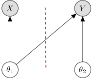
Rather than use the posterior (1), in possibly misspecified models it has been argued that we can cut the link between the modules to produce more reliable inferences for . This is the idea of cutting feedback; see Figure 1 for a graphical depiction of this “cutting” mechanism where, for simplicity, we assume does not depend on . In the case of the two module system, the cut (indicated by the vertical dotted line in Figure 1) severs the feedback between the modules and allows us to carry out inferences for based on module one, using the likelihood , and then inference for can be carried out conditional on . In the case of Bayesian inference, this philosophy has led researchers to conduct inference using the cut posterior distribution (see, Plummer, 2015, Jacob et al., 2017).
As shown in Carmona and Nicholls (2020) and Nicholls et al. (2022), the cut posterior is a “generalized” posterior distribution (see, e.g., Bissiri et al., 2016) that restricts the information flow to guard against model misspecification (Frazier and Nott, 2024). In the canonical two module system, the cut posterior takes the form
The common argument given for the use of instead of is the assumption that misspecification adversely impacts inferences for ; e.g., Liu et al. (2009), and Jacob et al. (2017). The cut posterior uses only information from the data in making inference about , ensuring inference is insensitive to misspecification of the model for . However, uncertainty about can still be propagated through for inference on via the conditional posterior .
Motivating example: HPV prevalence and cervical cancer incidence
We now discuss a simple example described in Plummer (2015) that illustrates some of the benefits of cut model inference. The example, which is discussed further in the supplementary material, is based on data from a real epidemiological study (Maucort-Boulch et al., 2008). Of interest is the international correlation between high-risk human papillomavirus (HPV) prevalence and cervical cancer incidence, for women in a certain age group. There are two data sources. The first is survey data on HPV prevalence for 13 countries. There are women with high-risk HPV in a sample of size for country , . There is also data on cervical cancer incidence, with cases in country in woman years of follow-up. The data are modelled as
The prior for assumes independent components with uniform marginals on . The prior for , assumes independent normal components, .
Module 1 consists of and (survey data module) and module 2 consists of and (cancer incidence module). The Poisson regression model in the second module is misspecified. Because of the coupling of the survey and cancer incidence modules, with the HPV prevalence values appearing as covariates in the Poisson regression for cancer incidence, the cancer incidence module contributes misleading information about the HPV prevalence parameters. The cut posterior estimates these parameters based on the survey data only, preventing contamination of the estimates by the misspecified module. This in turn results in more interpretable estimates of the parameter in the misspecified module, since summarizes the relationship between HPV prevalence and cancer incidence, but the summary produced can only be useful when the inputs to the regression (i.e. the HPV prevalence covariate values) are properly estimated.
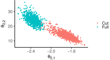
Figure 2 shows the marginal posterior distribution for for both the full and cut posterior distribution, which are very different, illustrating how the misspecification of the cancer incidence module distorts inference about HPV prevalence in the full posterior, resulting in uninterpretable estimation for . Further discussion of this example in the supplement shows the benefits of a semi-modular inference approach in which the tuning parameter interpolating between the cut and full posterior can be chosen based on a user-defined loss function reflecting the purpose of the analysis. A more complex real example is considered in Section 5.
2.2 The Impact of Misspecification in Modular Inference
In the remainder we consider a generalization of the canonical two-module system by assuming that the joint likelihood takes the form
where the individual models may or may not depend on the entire dataset . In the expressions above, and need not be densities as functions in so long as itself is a density; the terms and describe a decomposition of the likelihood having the dependence indicated by the arguments. The goal of modular Bayesian inference is to conduct inference on in the specific setting where inference for based only on is reasonable, but where the module contains additional useful information on ; see the regularity conditions in Appendix C.1 for specific details. Modular inference on can be carried out using the cut posterior
| (2) |
The cut posterior is beneficial when misspecification of makes full Bayesian inference on less accurate compared to Bayesian inference using only . The benefits of cutting feedback can be formalized by assuming that misspecification is limited to and that the true data generating process (DGP) has a density of the form111Strictly speaking, this analysis extends beyond density functions but we maintain the use of densities to simplify our discussion.
for some unknown component that controls the amount of model misspecification. The form of allows us to capture both gross model misspecification, and situations where misspecification is ambiguous. We first restrict our attention to gross model misspecification by imposing the following assumption.
Assumption 1 (Gross Misspecification).
The observed data is independent and identically distributed according to . For some , with , and all , for any . There exist that minimizes , the Kullback–Liebler divergence of over with respect to .
Under Assumption 1 and regularity conditions, the cut posterior can be shown to deliver accurate inferences for , while the full posterior does not. To state this result, denote the cut posterior distribution for as , and let denote the full posterior distribution for . For any , define . For the true data generating process, we say that (or ) if for all , as .
Lemma 1.
Assumption 1 embodies cases where a practitioner can confidently determine that the second module is misspecified. Lemma 1 then shows that, in these cases, the cut posterior concentrates on the true value , while the full posterior does not. By restricting the flow of information across modules, cutting feedback produces inferences for that are more accurate than full Bayesian inference. Although Lemma 1 implies that cut posterior inference is more accurate than full posterior inference when the second module is grossly misspecified, it is of limited use when and are similarly located, which can occur when misspecification of the second module is not severe. In such cases, the full posterior will have less uncertainty than the cut posterior, while also being similarly located, making it unclear whether to prefer the cut or full posterior.
To capture the empirically relevant setting where, for any fixed , it is unclear which posterior to use, we investigate the behavior of these posteriors under a certain class of locally misspecified DGPs. Following the literature of robust asymptotic statistical analysis (see, e.g., Ch 3. Rieder, 2012), we approximate the empirical situation where neither method is clearly preferable using a local perturbation about the assumed model:
| (3) |
which depends on a (random) direction of misspecification , and magnitude that takes values in . Under the local perturbation framework in (3) the cut and full posteriors have similar locations in for small-to-moderate sample sizes, and conventional specification testing methods cannot consistently detect which method delivers more accurate inferences for . As such, this class of perturbations allows us to compare cut and full posterior inference when correct specification of the second module is ambiguous.
Assumption 2 (Local Misspecification).
The triangular array is independent and identically distributed according to in (3) for fixed . For , compact, satisfies: (i) ; (ii) For partitioned conformably to , , and .
Remark 1.
Assumption 2 is a device that will allow us to rigorously compare the cut and full posteriors when neither is clearly preferable. The local misspecification framework ensures that, for any , there remains some ambiguity about model misspecification—and thus which posterior to prefer. It provides an appropriate theoretical framework for analyzing cut and full posteriors when the choice between them is unclear. Assumption 2 further maintains that the direction of misspecification, , does not adversely affect the location of the cut posterior for but will impact the full posterior.
Remark 2.
Assumption 2 resembles, but is distinct from, the misspecification device employed in Hjort and Claeskens (2003) and Claeskens and Hjort (2003) to construct methods that combine and choose between different frequentist point estimators. The approach outlined in Section 8 of Claeskens and Hjort (2003) is not appropriate here since their framework can produce cut posterior inferences for that are less accurate than the full posterior, which contradicts the underling reasoning for using cut posteriors. The misspecification framework in Assumption 2 also differs from the designs in Pompe and Jacob (2021), and Frazier and Nott (2024), which are similar to Assumption 1, and ensure that - with probability converging to one - the researcher knows the model is misspecified.
Under Assumption 2, cut posterior inference for is not impacted by misspecification of the second module. To show this, we require further notation. First, note that
where denotes the partial log-likelihood for used in the cut posterior, and denotes the log-likelihood used in the conditional posterior. Denote the derivative of the full log-likelihood as , and the second derivative by . For , define the first and second partial derivatives as , and . Similar notations will be use to denote derivatives of , for . Let denote the expectation of , under in Assumption 2, and define the following information matrices: , , and . Let , , and let denote weak convergence under .
Lemma 2.
(i) .
(ii) .
(iii) .
(iv) Only credible sets calculated under have valid frequentist coverage.
(v) The squared bias for and under is smaller than .
Remark 3.
Lemma 2 shows that inferences for using the cut posterior have no asymptotic bias, whereas the full posterior for has asymptotic bias and both posteriors have different biases for . The presence of asymptotic bias implies that, if , only credible sets for correctly quantify uncertainty, i.e., only has calibrated credible sets. Since the bias due to misspecification, , is unknown, it does seem feasible to determine whether or more reliably quantifies uncertainty in general, except when where both methods accurately quantify uncertainty.
Lemma 2 implies that the user is faced with a trade-off between conducting inference using the cut or full posterior: inferences under have the smallest variability possible (via Cramer-Rao) but exhibit a bias of unknown magnitude, whereas inferences under are guaranteed to have smaller bias than those under but have (weakly) larger variability. Lemma 2 is the first result to formally show that a bias-variance trade-off exists between the cut and full posteriors. Since the bias due to misspecification () is unobservable, Lemma 2 exemplifies the situation where it is ambiguous as to whether we should base inferences on the posterior that exhibits low bias - the cut posterior - or the posterior that exhibits larger bias but which has much smaller variability - the full posterior.
3 Semi-Modular Inference
Lemma 2 suggest that is we consider the accuracy of posteriors using a criteria that measures both the bias and variance of posterior inference, it should be possible to combine the cut and full posteriors to deliver inferences that are more accurate than using either by themselves. The goal of semi-modular inference (SMI) is to interpolate between the cut and full posteriors to reduce the uncertainty about while maintaining a tolerable level of bias. However, there are many ways to interpolate between two probability distributions, and there is no a priori reason to suspect one method of interpolation will deliver better results than others; see Nicholls et al. (2022) for a discussion on some of the possibilities.
Following Chakraborty et al. (2022) and Yu et al. (2023), we focus on conducting SMI using linear opinion pools (Stone, 1961), which produces a semi-modular posterior (SMP) that is a convex combination between the cut and full posteriors: for ,
| (4) | ||||
The pooling weight in the SMP determines the level of interpolation between the posteriors, and Chakraborty et al. (2022) suggest choosing using prior-predictive conflict checks, while Carmona and Nicholls (2022) propose to use out-of-sample predictive methods to select . In contrast, we propose a novel choice of pooling weight that leverages the bias-variance-trade-off between cut and full posterior inferences.
3.1 Shrinkage-based semi-modular posteriors
To build intuition as to how can utilize the bias-variance trade-off between and , we first focus on the behavior of the SMP for , i.e., in (4), and analyze the behavior of in subsequent sections.222Differences between the cut, full, and SMP posteriors for are attributable to differences in the posterior for since each posterior shares the same conditional posterior for given . Focusing on in (4), note that the SMP point estimator for is
| (5) |
where , and . From Lemma 2, the asymptotic mean of is zero, while that of depends on the misspecification bias . Hence, the SMP posterior mean combines an asymptotically unbiased estimator with high variance, , and an asymptotically biased estimator with small variance, . Therefore, if we are willing to tolerate some bias it will be possible to choose to deliver inferences on that are more accurate than either the cut or full posterior alone, at least so long as our measure of “accuracy” accounts for both bias and variance.
The idea of combining biased and unbiased estimators has a long history in statistics, with the most commonly encountered estimators of this kind being shrinkage and James-Stein estimators, see Chapter 5 of Lehmann and Casella (2006) for a textbook discussion. Indeed, the form of in (5) is reminiscent of those encountered in the shrinkage literature. For two normally distributed estimators, one biased and the other unbiased, Green and Strawderman (1991) demonstrated how to optimally combine such estimators to deliver a shrinkage estimator that is optimal in terms of expected squared error loss. The approach of Green and Strawderman (1991) was extended to more general settings and loss functions by Kim and White (2001), and Judge and Mittelhammer (2004).
While and are not normally distributed, they are asymptotically normal, and so one could choose in the SMP using existing shrinkage estimation proposals. Following ideas similar to Green and Strawderman (1991), and Kim and White (2001), we could choose in (4) as
| (6) |
for some , and a positive definite -matrix. Since is asymptotically biased, while is not, using within the SMP would allow us to interpret the SMP as shrinking cut posterior inferences towards those of the biased full posterior, and so using would deliver a type of “shrinkage” SMP (S-SMP).
Semi-modular Bayesian inference is clearly much more general than the linear Gaussian models analyzed in Green and Strawderman (1991), Kim and White (2001), and Judge and Mittelhammer (2004). Nevertheless, applying shrinkage estimation ideas within semi-modular Bayesian inference should allow us to effectively combine the cut and full posteriors. In the following sections, we show that this is indeed the case: empirically and theoretically, SMPs based on weights similar to (6) deliver inferences that can be shown to be optimal according to a general notion of asymptotic risk. Before presenting any formal analysis, we first illustrate the behavior of the S-SMP based on empirically in a simple example from the cutting feedback literature.
3.2 Example: Biased Mean
To demonstrate the benefits of the SMP, we consider a minor modification of the biased mean example in Section 2.1 of Liu et al. (2009). We observe two datasets generated from independent random variables with the same unknown mean , but where the assumed model for the second dataset is incorrect resulting in biased estimation of the parameter of interest. The first dataset corresponds to observations on a -dimensional, , random vector that we assume is generated from the model:
where and , , are iid . However, we also observe an additional dataset, comprised of observations which is assumed to be from the model:
where , , are iid for unknown . The prior density for is , and for is . The parameter of interest is , and we wish to determine how much the second dataset should influence inference about , when its assumed model is incorrect, leading to biased estimation of .333The original example of Liu et al. (2009) is such that for even moderate values of the bias we always prefer the cut posterior. Given this, we have slightly modified the original example to ensure a meaningful trade-off exists between the cut and full posteriors. Without this modification, the S-SMP simply returns the cut posterior in the vast majority of cases.
Suppose that in the actual data-generating process is not , but
for , where denotes a dimensional vector of ones. When , this reduces to the assumed model, but when we will obtain biased estimation of under the assumed model.
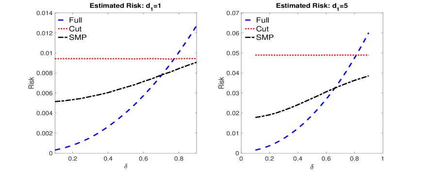
For our experiments, we assume and use an equally spaced grid of values for the contamination . For each value in this grid, we generate 1000 replications from the above process in the case where and , and consider two different values of . For each dataset, the S-SMP is based on the following version of the weights in (6): for and
To compare the impact of misspecification on the different modular posteriors we plot a Monte Carlo estimate of the expected squared error for the point estimators, based on 1000 replicated samples, across the grid of values for . The results are presented in Figure 3 and show that for relatively small levels of contamination, the full posterior has lower expected squared error than the cut posterior, due to having a much smaller variance, while at higher levels of contamination the cut posterior has lower expected squared error. However, the expected squared error for the S-SMP is always lower than the cut posterior, which demonstrates that the SMP is able to ‘trade-off’ between the two posteriors to minimize squared error risk across all levels of contamination. However, we note that when and , the S-SMP and cut posterior give very similar results.444Appendix D in the supplementary material contains additional experiments for this example. These results show that the S-SMP delivers reasonable results for all choices of and becomes more accurate as the dimension increases.
4 Measuring posterior accuracy through risk
The example in Section 3.2 suggests that the S-SMP can deliver more accurate inferences, in terms of expected squared error, than the cut or full posterior. This generally suggests that the S-SMP can deliver inferences that are accurate according to a criteria that measures both the bias and variance of posterior inferences. However, we remark that such a notion of accuracy is only one way to measure the accuracy of posterior inferences. In modular Bayesian inference, Jacob et al. (2017) and Pompe and Jacob (2021) have suggested choosing between full and cut posteriors using out-of-sample predictive accuracy, while Carmona and Nicholls (2020) have suggested a similar approach for calibrating an SMI tuning parameter. While such an approach is undoubtedly useful, the empirical analysis in Jacob et al. (2017), as well as the empirical and theoretical analysis in Pompe and Jacob (2021), suggest that the preferred method according to such criteria is example specific, with neither method likely to be generally preferable. Further, Lemma 2 demonstrates that cut and full posterior inferences for exhibit asymptotic bias, and it is not clear how notions of predictive accuracy account for the impact of this bias on the resulting inferences.
In contrast to predictive approaches, we propose to measure the accuracy of modular and semi-modular posteriors through an inferential criterion that can accounts for both the bias and variance in the resulting inferences. Given that the SMP includes the cut () and full posterior () as special cases, we evaluate the accuracy of different posteriors using the “posterior risk” associated to different values. This notion of risk has previously been used by Castillo (2014) and Lee and Lee (2018) to choose between different prior classes in Bayesian inference, and is capable of capturing both the bias and variance associated with posterior inferences.
Given a user-chosen loss function , at the point we can measure the loss associated with via the posterior risk . For recall that , with as in Assumption 2. The trimmed Posterior risk of at (hereafter, referred to simply as P-risk) is defined as:555Trimming is necessary to ensure that the expectation exists, and can be disregarded in practical terms.
The loss function satisfies the following assumptions.
Assumption 3.
For all , the loss function satisfies: i) and if and only if ; ii) The loss is absolutely continuous in , and three times continuously differentiable in ; iii) For in a neighbourhood of , the matrix is continuous, and positive semi-definite; iv) For each , and for all , , , where denotes the -th direction of , and .
Remark 4.
Assumption 3 includes losses such as squared error loss , but also permits intrinsic measures of accuracy for densities. The Kullback-Liebler divergence,
and various scoring rules, such as kernel scores or mean-variance scores (see Gneiting and Raftery, 2007, Sections 4 and 5), will satisfy Assumption 3. Assumption 3 does exclude discontinuous functions, such as those needed to measure the accuracy of quantiles. Extending our results to the case of discontinuous losses is the focus of subsequent work by the authors.
P-risk is related to expected asymptotic risk, which is often used to gauge the accuracy of frequentist point estimators. Since is calculated from a chosen posterior based on a decision made for , we refer to this notion as P-risk to distinguish it from asymptotic risk. Risk has a long history in statistical analysis and we refer to Chapter 6 of Lehmann and Casella (2006), and Chapter 8 of Van der Vaart (2000) for textbook treatments. The key benefit of using P-risk to measure different choices for is that, for the chosen loss , P-risk can deliver a concrete ranking across inference procedures relative to this choice. Furthermore, our use of P-risk is not at odds with Bayesian inference, and has already been used by others, albeit in slightly different contexts. More generally, as argued by Lehmann and Casella (2006) (pg 310): “The Bayesian paradigm is well suited for the construction of possible estimators, but is less well suited for their evaluation.” Consequently, we follow this suggestion of Lehmann and Casella (2006) and carry out inference via Bayesian methods but evaluate the accuracy of these methods using our notion of asymptotic risk (i.e., P-risk).
4.1 The P-risk of SMPs
As we have already seen in Section 3.1, weights of the form presented in (6) deliver a SMP whose expected squared error was smaller than the cut posterior. Thus, in the remainder we focus our theoretical analysis on SMPs with pooling weights that are general versions of those in (6): for a user-chosen sequence such that , , define the pooling weight
| (7) |
In contrast to the weight suggested in (6), the weight in (7) depends on the entire vector , and the curvature of the loss function, as captured by the matrix . Incorporating the curvature of the loss within the pooling weight is necessary for the SMPs to deliver inferences that are accurate according to the chosen loss; see Theorem C.3 of Appendix C.3 for further discussion.
The pooling weight in (7) yields the shrinkage SMP (S-SMP):
| (8) |
Different choices of in (7) deliver different weights and ultimately different posteriors. However, the following result shows that across a range of choices for , the P-risk of in (8) is dominated by that of the cut posterior, and, under certain conditions, that of the full posterior. To state this result simply, define the -dimensional matrix , and denote the -block of by (see Assumption 3); let be a matrix with -block , -block , and -block , where . We remind the reader that , () and are defined in Section 2.2.
Theorem 1.
(i)
(ii) for .
Remark 5.
Under the class of misspecified DGPs in Assumption 2 and in terms of P-risk, Theorem 1 demonstrates that the cut posterior delivers a point estimator that is inadmissable, with a similar results also being true for the full posterior under additional conditions. Hence, from the standpoint of P-risk, the S-SMP is preferable to the cut posterior and under certain conditions the full posterior as well. However, it is unclear if the S-SMP has the lowest possible P-risk, i.e., if it is minimax. Answering this question requires deriving a local minimax efficiency bound for the class of DGPs in Assumption 2 (see, e.g., Chapter 8 in Van der Vaart, 2000 for a discussion on asymptotic minimax estimators), which is outside the scope of the current paper, and is left for future research.
Remark 6.
As suggested by an anonymous referee, a Bayesian may also be interested in the uncertainty quantification of the S-SMP. As discussed in Remark 3 after Lemma 2, only credible sets based on deliver calibrated uncertainty quantification. Therefore, if the credible sets of the S-SMP will not be calibrated. More generally, the credible sets calculated from the cut posterior, full posterior and S-SMP all depend, in different ways, on the magnitude of the bias induced via misspecification. Since is unknown in practice it is not obvious how one should theoretically compare the behavior of such credible sets. In light of this issue, we believe that measuring the accuracy of the posteriors using P-risk is the most direct approach.
Remark 7.
The condition in Theorem 1 is related to the inefficiency that results from using the cut posterior relative to the full posterior. This condition is more likely to be satisfied when the efficiency gap between the cut and full posterior is large, or when - the dimension of - is large. That being said, the condition is a sufficient condition and it is possible that the S-SMP may deliver smaller P-risk even when this condition is not satisfied.
Remark 8.
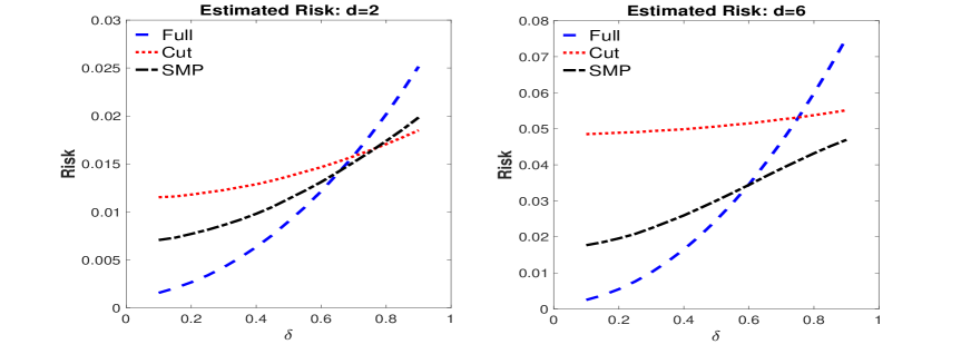
The example in Section 3.2 demonstrated that a S-SMP focused on inference for delivered smaller expected P-risk for than the cut posterior. However, Theorem 1 makes clear that the S-SMP can also deliver smaller P-risk for . Returning to the example in Section 3.2, we now analyze the P-risk at for the S-SMP under the shrinkage weight
To this end, we repeat the Monte Carlo experiment in Section 3.2 under two different dimensions for , so that , and present the results in Figure 9. These results show that the P-risk of the S-SMP is dominated by that of the cut posterior, and in certain cases that of the full posterior; as with the example in Section 3.2, for , and , the S-SMP and cut posterior give very similar results. Theorem 1 is asymptotic and given the sample sizes considered in this experiment it is not surprising that at large levels of contamination the S-SMP can perform slightly worse than the cut posterior (when ), since non-negligible weight is placed on the full posterior. However, at the median pooling weight across the replications is about , so that most of the pooling weight corresponds to the cut posterior. As we shall see shortly, under higher levels of misspecification and as increases, the S-SMP resembles the cut posterior.
Part one of Theorem 1 implies that if the cut posterior is inefficient relative to the full posterior, as measured by , then the S-SMP will be at least as accurate (in P-risk) as the cut posterior, and potentially more accurate than the full posterior.666Theorem 1 applies even if : when there is no misspecification bias the cut and full posterior means will be similar and the weight will be close to unity so that the S-SMP will resemble the full posterior. The second part of Theorem 1 gives a sufficient, but not necessary, condition which guarantees that the P-risk of the full posterior dominates that of the S-SMP. This condition is likely to be satisfied when the difference in posterior locations is larger than the difference in posterior variances.
When it is also possible to obtain an analytic expression for the P-risk of the S-SMP if we set , so that . The requirement that is commonly encountered in the risk analysis of James-Stein estimators and is a consequence of the fact that can be viewed as performing a type of posterior shrinkage.
Theorem 2.
Theorem 2 is useful as it gives an exact bound on the P-risk, and an easily interpretable set of conditions for the value of in the weight . Under , the condition is necessary to guarantee that has smaller P-risk than . This condition is related to Stein’s phenomenon (see Ch. 6 of Lehmann and Casella, 2006 for a discussion) and implies that using the cut posterior by itself is sub-optimal (in terms of P-risk) when . We stress that this interpretation is only valid when and that a similar phenomena does not necessarily extend to other loss functions.
Theorems 1-2 demonstrate that, under certain conditions and in terms of P-risk, the S-SMP is more accurate than the cut posterior and possibly the full posterior. However, Theorems 1-2 implicitly require that the difference between the cut and full posterior locations do not diverge, which is a consequence of the asymptotic regime in Assumption 2. This begs the question of what happens to the S-SMP when we move from the case of local model misspecification (Assumption 2) to gross model misspecification (Assumption 1). The following result demonstrates that under gross model misspecification the S-SMP converges to the cut posterior, and so is robust to either form of misspecification.
5 Additional examples
5.1 Normal-normal random effects model
We first apply the S-SMP to the misspecified normal-normal random effects model presented in Liu et al. (2009). The observed data is comprising observations on groups, with observations in each group, which we assume are generated from the model , with random effects . The goal of the analysis is to conduct inference on the standard deviation of the random effects, , and the residual standard deviation parameters . Below we write , and .
For and , , the likelihood for can be written to depend only on the sufficient statistics and , where independently for ,
Letting and , the random effects model can then be written as a two-module system of the form shown in Figure 1: module one depends on , , and module two depends on , .
Let denote the value of the density evaluated at , and denote the value of the density evaluated at . The first module has likelihood , while the second module has likelihood .
When the Gaussian prior for the random effects term conflicts with the likelihood information, inferences for can be adversely impacted. Such an outcome will happen when, for instance, a value of differs markedly from its assumed model. Liu et al. (2009) argue that the thin-tailed Gaussian assumption for the random effects can produce poor inferences for due to the feedback induced by the likelihood term in the second module. To guard against this Liu et al. (2009) propose cut posterior inference for , which can be accommodated by simply updating the posterior for using only the information in the corresponding summary statistics : given , and independent across , the cut posterior for (where this denotes the elementwise square of ) is
Summaries of the cut posterior for can be obtained by sampling from the cut posterior for and transforming the samples. Joint inferences for can be carried out using the cut posterior distribution
where the conditional posterior is obtained from the joint posterior for .
We now demonstrate that the S-SMP delivers inferences for that are more accurate than the cut posterior for different levels of misspecification. We generate 500 repeated samples from the normal-normal random effects model with groups each with random effect component , . For each group, we set and . We induce model misspecification through the random effect term . Following the design of Liu and Goudie (2022b) we induce misspecification by forcing to be an outlier, however, unlike Liu and Goudie (2022b) we consider that the magnitude of the outlier decreases as the number of individual observations in each group, , increases. We set the random effect for the first group as , and consider . When is small the cut posterior delivers more accurate inferences for than the full posterior as the feedback between this outlier and has been removed. As the magnitude of the outlier shrinks, the full posterior for become more accurate and a meaningful trade-off between the cut and full posteriors exists.
Our goal is to measure the impact of misspecification on the inferences for , and so we choose the weight in the S-SMP using squared error loss for this component only. This produces a pooling weight that is similar to that discussed in Section 3.2 but based on and not the entire vector of .777Since only the first random effect component, , is misspecified, inferences for are not impacted by misspecification. In this way, even if the pooling weight was estimated based on the entire vector for it would be the component that would drive the pooling weight since the posterior means for the cut and full posterior are very similar for the remaining components. We present Monte Carlo estimates (calculated over the 500 replicated datasets) of the corresponding P-risk under squared error loss for the posteriors in Table 1. Across all values of , the S-SMP has smaller P-risk than the cut posterior, and in many cases the full posterior as well. Further, the cut posterior is more accurate than the full posterior when is small but the full posterior becomes more accurate as increases. In this way, the weight in the S-SMP is close to unity with small , but increases as increases. However, for large the cut and full posteriors behave similarly, and the S-SMP maintains most of the weight on the cut posterior.
| 10.5365 | 2.9705 | 1.1753 | 0.3723 | 0.1897 | |
| 8678.9763 | 4.6894 | 1.3124 | 0.5491 | 0.2634 | |
| 10.5365 | 3.5806 | 1.4721 | 0.5102 | 0.2581 | |
| 0.00 | 0.18 | 0.23 | 0.15 | 0.15 |
5.2 Archaeological example
Our final example, discussed in Styring et al. (2017), Carmona and Nicholls (2020) and Yu et al. (2023), involves data collected to evaluate an “extensification hypothesis” for early Mesopotamian agricultural practices. The hypothesis states that as cities grew, agriculture extended over larger areas with less intensive cultivation, rather than more intensively farming existing areas to meet food demands.
The analysis uses two data sources: an archaeological dataset and a modern experimental dataset. Figure 5, which is similar to Figure 6 from Carmona and Nicholls (2020), shows a graphical representation of the model which comprises two modules. The first, the “HM module”, is a Gaussian linear regression model incorporating random effects. The second, the “PO module”, is a proportional odds model used to impute a missing categorical covariate for the HM module.
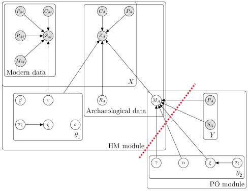
In the HM module’s regression, the response is nitrogen level of cereal grains, denoted . We follow the notation of Yu et al. (2023) and use subscripts of and to denote archaeological and modern values of any variable. So, for example, and are nitrogen levels of cereal grains for archaeological and modern data respectively. For covariates in the HM module we have crop category , site location (a categorical variable), site size , rainfall and manure level . Archaeological data for rainfall and manure level, and , are missing. The HM module is a linear regression model with fixed effects for rainfall and manure level, a random effect for site location, and error variance based on crop category.
The imputation model in the PO module imputes the missing manuring level covariates for the archaeological data with parameters . The prior on is a proportional odds model with covariates site size and site location. The parameter is the site size coefficient; a negative supports the extensification hypothesis. The parameter is a vector of random effects for five archaeological site locations in the proportional odds model, is the standard deviation of random effects, and is a vector of two threshold parameters. Further details on the model and priors are available in Appendix B.1 of Yu et al. (2023). Bayesian modular inference is relevant in this example because the PO module may be poorly specified. Therefore, we can cut feedback so that is imputed based solely on the hierarchical model for cereal grain nitrogen levels (HM module in Figure 5), ensuring that imputation of and the interpretation of are unaffected by any misspecification in the PO module.
In Figure 5, the red line indicates a “cut” between the modules. Figure 6 provides a simplified model structure.
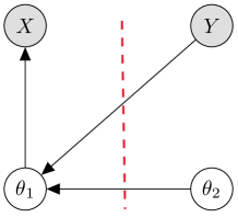
Although it looks different from the two-module system in Figure 1, the cut posterior has the same form, allowing cut and semi-modular inference to proceed similarly. Here we consider how semi-modular inference changes according to the choice of the loss function. For a given scalar parameter , we will consider a S-SMP posterior using mixing weight
where and are the cut and full marginal posterior variances for , and and are the cut and full marginal posterior means for . This is similar to the S-SMP in Section 3.2, but based on the marginal full and cut posteriors for .
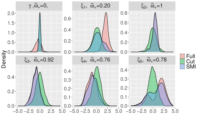
Figure 7 shows the cut, full and S-SMP posteriors for (the parameter of main interest) and the proportional odds regression random effects . When basing the mixing weight on (top left), we do a full cut, while basing the mixing weights on results in mixing weights varying between and . In this example, the shrinkage weight can vary a great deal depending on what scalar parameter is being targeted in the loss function, and so the use of an appropriately defined loss function for the application is crucial. The S-SMP for shows weaker evidence for the extensification hypothesis than the standard posterior, in the sense that the posterior probabililty of is smaller. Details of the MCMC approach for generating samples from the cut posterior, as well as an SMC method to generate samples from the full posterior, are given in Yu et al. (2023).
6 Discussion
Choosing between the cut and full posteriors is difficult when model misspecification is not severe and in such cases semi-modular posteriors (SMPs) proposed in Carmona and Nicholls (2020) are an attractive alternative. While SMPs are motivated by the presence of a bias-variance trade-off between cut and full posterior inferences, this paper is the first to formalize the existence of such a trade-off. Using SMPs based on linear opinion pooling, we devise a novel pooling weight that allows the SMP to leverage this bias-variance trade-off. Our proposed shrinkage SMP is simple to implement and possess useful theoretical guarantees that other SMP approaches do not posses: the posterior risk of our shrinkage SMP is dominated by that of the cut posterior, and, under certain conditions, that of the full posterior. An interesting future direction would be to determine if our theoretical results can be extended to other types of SMPs, such as those of Carmona and Nicholls (2020) and Nicholls et al. (2022).
As suggested by a referee, the notion of asymptotic risk we consider is only one criterion with which to judge the accuracy of posterior inferences, with posterior predictive accuracy and the validity of posterior credible sets being alternative measures. While assessing the accuracy of different methods based on posterior predictive accuracy is empirically feasible, it is not obvious that it is feasible to deduce a ranking across different modular Bayesian methods under our maintained assumptions. Further, the random weighting of the SMP ensures that determining the asymptotic shape of this posterior, and thus the behavior of its credible sets, is not straightforward. We leave these interesting topics for future study.
Acknowledgments
David T. Frazier gratefully acknowledges support by the Australian Research Council through grant DE200101070. David Nott’s research was supported by the Ministry of Education, Singapore, under the Academic Research Fund Tier 2 (MOE-T2EP20123-0009). We thank seminary participants at the Weierstrass Institute for Applied Analysis and Stochastics, and the Computational methods for unifying multiple statistical analyses (Fusion) workshop for helpful comments. In addition, we thank Pierre Jacob for helpful comments on some of the stated results. The authors also thank the associate editor and referees for very helpful comments that significantly improved the paper.
References
- Bennett and Wakefield (2001) Bennett, J. and J. Wakefield (2001). Errors-in-variables in joint population pharmacokinetic/pharmacodynamic modeling. Biometrics 57(3), 803–812.
- Bissiri et al. (2016) Bissiri, P. G., C. C. Holmes, and S. G. Walker (2016). A general framework for updating belief distributions. Journal of the Royal Statistical Society. Series B, Statistical methodology 78(5), 1103.
- Blangiardo et al. (2011) Blangiardo, M., A. Hansell, and S. Richardson (2011). A Bayesian model of time activity data to investigate health effect of air pollution in time series studies. Atmospheric Environment 45(2), 379–386.
- Carmona and Nicholls (2020) Carmona, C. and G. Nicholls (2020). Semi-modular inference: enhanced learning in multi-modular models by tempering the influence of components. In International Conference on Artificial Intelligence and Statistics, pp. 4226–4235. PMLR.
- Carmona and Nicholls (2022) Carmona, C. and G. Nicholls (2022). Scalable semi-modular inference with variational meta-posteriors. arXiv:2204.00296.
- Carpenter et al. (2017) Carpenter, B., A. Gelman, M. D. Hoffman, D. Lee, B. Goodrich, M. Betancourt, M. Brubaker, J. Guo, P. Li, and A. Riddell (2017, January). Stan: A Probabilistic Programming Language. Journal of Statistical Software 76(1), 1–32. Number: 1.
- Castillo (2014) Castillo, I. (2014). On Bayesian supremum norm contraction rates. Annals of Statistics.
- Chakraborty et al. (2022) Chakraborty, A., D. J. Nott, C. Drovandi, D. T. Frazier, and S. A. Sisson (2022). Modularized Bayesian analyses and cutting feedback in likelihood-free inference. Statistics and Computing (To appear).
- Claeskens and Hjort (2003) Claeskens, G. and N. L. Hjort (2003). The focused information criterion. Journal of the American Statistical Association 98(464), 900–916.
- Davidson (1994) Davidson, J. (1994). Stochastic limit theory: An introduction for econometricians. OUP Oxford.
- Frazier and Nott (2024) Frazier, D. T. and D. J. Nott (2024). Cutting feedback and modularized analyses in generalized Bayesian inference. Bayesian Analysis 1(1), 1–29.
- Gneiting and Raftery (2007) Gneiting, T. and A. E. Raftery (2007). Strictly proper scoring rules, prediction, and estimation. Journal of the American statistical Association 102(477), 359–378.
- Green and Strawderman (1991) Green, E. J. and W. E. Strawderman (1991). A James-Stein type estimator for combining unbiased and possibly biased estimators. Journal of the American Statistical Association 86(416), 1001–1006.
- Grünwald and Van Ommen (2017) Grünwald, P. and T. Van Ommen (2017). Inconsistency of Bayesian inference for misspecified linear models, and a proposal for repairing it. Bayesian Analysis 12(4), 1069–1103.
- Hansen (2016) Hansen, B. E. (2016). Efficient shrinkage in parametric models. Journal of Econometrics 190(1), 115–132.
- Hjort and Claeskens (2003) Hjort, N. L. and G. Claeskens (2003). Frequentist model average estimators. Journal of the American Statistical Association 98(464), 879–899.
- Jacob et al. (2017) Jacob, P. E., L. M. Murray, C. C. Holmes, and C. P. Robert (2017). Better together? Statistical learning in models made of modules. arXiv preprint arXiv:1708.08719.
- Jacob et al. (2020) Jacob, P. E., J. O’Leary, and Y. F. Atchadé (2020). Unbiased Markov chain Monte Carlo methods with couplings. Journal of the Royal Statistical Society: Series B (Statistical Methodology) 82(3), 543–600.
- Judge and Mittelhammer (2004) Judge, G. G. and R. C. Mittelhammer (2004). A semiparametric basis for combining estimation problems under quadratic loss. Journal of the American Statistical Association 99(466), 479–487.
- Kim and White (2001) Kim, T.-H. and H. White (2001). James-Stein-type estimators in large samples with application to the least absolute deviations estimator. Journal of the American Statistical Association 96(454), 697–705.
- Kleijn and van der Vaart (2012) Kleijn, B. and A. van der Vaart (2012). The Bernstein-von-Mises theorem under misspecification. Electron. J. Statist. 6, 354–381.
- Lee and Lee (2018) Lee, K. and J. Lee (2018). Optimal Bayesian minimax rates for unconstrained large covariance matrices. Bayesian Analysis.
- Lehmann and Casella (2006) Lehmann, E. L. and G. Casella (2006). Theory of point estimation. Springer Science & Business Media.
- Liu et al. (2009) Liu, F., M. Bayarri, and J. Berger (2009). Modularization in Bayesian analysis, with emphasis on analysis of computer models. Bayesian Analysis 4(1), 119–150.
- Liu and Goudie (2022a) Liu, Y. and R. J. B. Goudie (2022a). A general framework for cutting feedback within modularized Bayesian inference. arXiv:2211.03274.
- Liu and Goudie (2022b) Liu, Y. and R. J. B. Goudie (2022b). Stochastic approximation cut algorithm for inference in modularized Bayesian models. Statistics and Computing 32(7).
- Liu and Goudie (2023) Liu, Y. and R. J. B. Goudie (2023). Generalized geographically weighted regression model within a modularized Bayesian framework. Bayesian Analysis (To appear).
- Lunn et al. (2009) Lunn, D., N. Best, D. Spiegelhalter, G. Graham, and B. Neuenschwander (2009). Combining MCMC with ‘sequential’ PKPD modelling. Journal of Pharmacokinetics and Pharmacodynamics 36, 19–38.
- Maucort-Boulch et al. (2008) Maucort-Boulch, D., S. Franceschi, and M. Plummer (2008). International correlation between human papillomavirus prevalence and cervical cancer incidence. Cancer Epidemiology and Prevention Biomarkers 17(3), 717–720.
- Miller (2021) Miller, J. W. (2021). Asymptotic normality, concentration, and coverage of generalized posteriors. Journal of Machine Learning Research 22(168), 1–53.
- Newey (1985) Newey, W. K. (1985). Maximum likelihood specification testing and conditional moment tests. Econometrica: Journal of the Econometric Society, 1047–1070.
- Nicholls et al. (2022) Nicholls, G. K., J. E. Lee, C.-H. Wu, and C. U. Carmona (2022). Valid belief updates for prequentially additive loss functions arising in semi-modular inference. arXiv preprint arXiv:2201.09706.
- Plummer (2015) Plummer, M. (2015). Cuts in Bayesian graphical models. Statistics and Computing 25(1), 37–43.
- Pompe and Jacob (2021) Pompe, E. and P. E. Jacob (2021). Asymptotics of cut distributions and robust modular inference using posterior bootstrap. arXiv preprint arXiv:2110.11149.
- Rieder (2012) Rieder, H. (2012). Robust Asymptotic Statistics: Volume I. Springer Science & Business Media.
- Rousseau (1997) Rousseau, J. (1997). Asymptotic bayes risks for a general class of losses. Statistics & probability letters 35(2), 115–121.
- Shen and Wasserman (2001) Shen, X. and L. Wasserman (2001). Rates of convergence of posterior distributions. The Annals of Statistics 29(3), 687–714.
- Stone (1961) Stone, M. (1961). The opinion pool. The Annals of Mathematical Statistics, 1339–1342.
- Styring et al. (2017) Styring, A., M. Charles, F. Fantone, M. Hald, A. McMahon, R. Meadow, G. Nicholls, A. Patel, M. Pitre, A. Smith, A. Sołtysiak, G. Stein, J. Weber, H. Weiss, and A. Bogaard (2017). Isotope evidence for agricultural extensification reveals how the world’s first cities were fed. Nature Plants 3, 17076.
- Van der Vaart (2000) Van der Vaart, A. W. (2000). Asymptotic statistics, Volume 3. Cambridge University Press.
- Yu et al. (2023) Yu, X., D. J. Nott, and M. S. Smith (2023). Variational inference for cutting feedback in misspecified models. Statistical Science 38(3), 490–509.
Appendix A Supplementary Material
This supplementary material contains the regularity conditions used to obtain the results in the main text, proofs of all stated results and several lemmas used to prove the main results. The regularity conditions and proofs are broken up into two sections that depend on whether the analysis is conducted under gross model misspecification (Assumption 1), or local model misspecification (Assumption 2). In addition, this material contains further details of the HPV and cervical cancer incidence example introduced in Section 2.1 of the main text, and additional experiments for the biased means example in Section 3.2.
Appendix B Gross Misspecification: Assumption 1
B.1 Regularity Conditions
The regularity conditions used to prove Lemma 1 are similar to those used to deduce posterior concentration rates in generalized Bayesian methods; see, e.g., Shen and Wasserman (2001), as well as Miller (2021). We state the assumptions separately for the cut posterior and the full posterior. Recall, , and rewrite the cut posterior for as
For , write so that . For , define .
Assumption B1.
The following are satisfied.
-
(i)
For any there exists and a sufficiently large such that
-
(ii)
For all , , and ,
-
(iii)
For , , .
-
(iv)
For any , if , then with positive probability.
Remark 9.
Assumptions B1 parts (i), (iii) are identical to those maintained in Shen and Wasserman (2001) but for the partial log-likelihood , while the bound on the posterior denominator in Assumption B1(ii) is maintained to simply the proofs and can be removed at the cost of additional technicalities; for instance, using arguments similar to those of Lemma 1 in Shen and Wasserman (2001).
From the definition of ,
Setting minimizes the first part of , but does not minimize both components. Hence, under Assumption 1, is the value we would expect the full posterior to concentrate onto as . Thus, conducting joint Bayesian inference on under Assumption 1 results in posteriors for which will not concentrate onto . To formally prove this result, recall the definition , and consider the following regularity conditions, which are equivalent version of Assumption B1 but for , and .
Assumption B2.
The following are satisfied.
-
(i)
For any there exists and a sufficiently large such that, for some ,
-
(ii)
For all , , , and ,
-
(iii)
For , , and .
-
(iv)
For any , if , then with positive probability.
B.2 Proofs of Main Results: Gross Misspecification
Proof of Lemma 1.
We prove the two cases separately, starting with the cut posterior.
Part 1: Cut posterior.
For , recall , and consider
Apply Assumption B1(ii) to see that, with probability at least ,
| (9) |
where the last term follows by Assumption B1(iii).
Focus on the term in brackets in (9). Since is bounded for any finite , the log-likelihood ratio is also bounded for any , and so by Assumption B1(i),
with probability converging to one (since for all ).
Part 2: Exact posterior. Repeating similar arguments to those above, but for the set , proves that, with probability converging to one
However, defining , since , it follows that
Hence, with probability converging to 1, . Since under Assumption 1, there exists some , such that , so that for any , in probability. ∎
Proof of Corollary 1.
Write the SMP as
| (10) |
where . Apply (10), and Fubini, to obtain
We can then write
The stated result now follows if as .
To show this, let , , and . Then, for ,
By the reverse triangle inequality
By the hypothesis of the result, , while under Assumption 1, , so that as , and the stated result follows. ∎
Appendix C Local Misspecification: Assumption 2
C.1 Regularity Conditions: Local Misspecification
Before stating the regularity conditions we maintain in this section, we recall several notations previously defined in the main text. Let , and denote the joint log-likelihood for the -th observation as . Denote the full derivative of the log-likelihood as , and denote the second derivative as . For , define the partial derivatives , and the second partial derivatives . For a function , let denote the expectation of under in Assumption 2; i.e., . Define the matrices , and . Recall that in Assumption 2 is partitioned conformably with .
In addition, note that
where signifies the ‘partial log-likelihood’ term, and signifies the log-likelihood term that is used in cut inference to construct the conditional posterior for given . Define the partial derivatives of as , , and recall . For and , define and . From the structure of the log-likelihood , note that
To formalize the impact of the misspecification in Assumption 2, we impose the following regularity conditions on the density .888We eschew measurability conditions and assume that all objects written are measurable.
Assumption C1.
For , let , be elements of the interior of , where and compact. The function is twice continuously differentiable in for almost all . There exist positive functions , such that for all , except on sets of measure zero, , satisfies the following: , and for all , and some , each of the following , , are less than . Further, , and the set does not depend on .
In addition, we maintain the following assumptions about the assumed model .
Assumption C2.
For any , if , then with positive probability.
C.2 Preliminary Results
The following intermediate results are used to state and prove our main results.
Lemma C.1.
The following Lemma is used to prove the results under the drifting sequences of DGPs constructed in Assumption 2.
Lemma C.2.
Lemma C.3.
The following is a useful extension of Stein’s Lemma.
Lemma C.4 (Lemma 2 of Hansen, 2016).
If is an vector, and is matrix, for continuously differentiable, then for ,
| (11) |
To simplify proofs of our results, we use the following block-matrix notations: for , let denote a matrix of zeros, and define
In addition, define
where we note that and have dimension . Recall
When no confusion is likely to result, when terms are evaluated at , we drop their dependence on this value; e.g., for we will often write .
Lemma C.5.
To analyze the behavior of the S-SMP, we must first deduce the behavior of and . To this end, define the statistics
which are partitioned conformably with . Define
The cut and full posteriors for and are given by
Theorem C.2.
Corollary C.1.
Remark 11.
We do not explicitly consider that the cut and full posteriors are computed from samples of different sizes; e.g., for the exact and for the cut. While useful, this difference in sample sizes will not have a significant impact on the resulting behavior of the SMP so long as . If one wishes to impose such a condition, the only result will be a slight change in the definition of the matrix in Lemma C.5 to account for the fact that . As such, all results presented herein can be extended to this case at the cost of minor additional technicalities. To see this, let be the larger sample size associated with the full posterior, and the smaller sample size associated with the cut posterior, which satisfies for some . Then, our results go through with since
where the second equality follows from Theorem C.2 (when is based on observations).
C.3 Proofs of Main Results
Recall the definitions , and
| (12) |
To prove Theorem 1 in the main text, we first prove the following result.
Theorem C.3.
Proof of Theorem C.3..
For , and , following arguments similar to those in Theorem 1 of Rousseau (1997), it can be shown that
and similarly (under Assumption 2),
which together imply that
Write
By Lemma C.6,
where , and are defined in Lemma C.5, and where
For , and , let
By Theorem 1.8.8 of Lehmann and Casella (2006),
For , the RHS of the above converges to , and we have that
Expand :
From the definitions of ,
Let us concentrate our attention on the last term in . Define the mapping and note that
Recall that , and . Using Lemma C.4, and for , we have
| (13) |
From the properties of , and Lemma C.5,
For the second term in (13), we have that
and where the last equality again follows from Lemma C.5. Consequently, for positive semi-definite,
| (14) |
where the last inequality holds for any matrix norm such that if and are positive semi-definite, then ; e.g., the Frobenius norm. Applying (14) into (13), we have
| (15) |
Applying (15) into the last equation for , and collecting terms yields
| (16) |
∎
Theorem C.3 yields the following corollary.
Corollary C.2.
Proof of Corollary C.2..
Since is Gaussian with mean zero and variance ,
| (18) |
From equation (16) in the proof of Theorem C.3,
where the second inequality follows by Jensen’s inequality, and the second to last by plugging in the moment of the quadratic form in equation (18), while the last (strict) inequality follows since .
Proof of Theorem 1 (main text)..
Theorem 1 is a direct consequence of Corollary C.2. To see this, note that Corollary C.2 is true pointwise for any such that . Note that and are convex for all , and that the RHS of the bound for in equation (17) is also convex as a function of . Hence, Corollary C.2 holds uniformly, which verifies Theorem 1. ∎
Proof of Theorem 2.
Recall the expanded expression for in the proof of Theorem C.3. Recall equation (13) derived in that proof of Theorem C.3:
where . Under our choice of loss, we can show that
For the second term in (13),
Applying the above, the second term in (13) becomes
| (19) |
From Lemma C.5, Hence, the inverse of the random variable in (19) is distributed as non-central chi-squared with degrees of freedom, and non-centrality parameter , which, for , has density function
To calculate , first we see that
and note that, since , when , for all ,
so that we can rewrite the expectation as
Taking then yields the result. ∎
C.4 Proofs of Preliminary Results in Section C.2
When no confusion is likely to result, quantities that are evaluated at will have their dependence on suppressed; i.e., we write , etc.
Proof of Lemma C.1..
Note that, under the regularity conditions in Assumption C1, we can exchange the order of integration and differentiation. Furthermore, note that for as in Assumption 2 and , we have that
where recall that
Similarly, from the structure of the score equations, and the information matrix equality, we have that
Analysing the above we see that
| (20) |
where the last line follows from rewriting , and from exchanging integration and differentiation to note that the second term is zero. This proves part one of the result. Repeating the argument for for yields
which proves the second part of the result.
Now, let us investigate the equivalence of each term. For the first term we have that
| (21) |
Applying the above equations for , , in equation (21) we have
which is satisfied if and only if . Hence, we have part three of the stated result.
Lastly, we investigate the term . Again, using the definitions of this term we have
| (22) |
where the last equality again follows from exchanging integration and differentiation of the second term, and rewriting the derivatives in the first term. Therefore, from equation (22), and the general matrix information equality, we have the equality
which is satisfied if and only if , which proves the last result. ∎
Proof of Lemma C.2.
To simplify the proof, let . By Assumption C1, under Assumption 2, we see that . By Assumption 2, there exists some with such that . Hence, for each , and . From Assumption C1, we have that , and . By the dominated convergence theorem, we then have that exists for each .
To prove the second part of the result, we note that, by Assumption 2,
| (23) |
where the second line follows since by Assumption C1 .
Now, by the triangle inequality,
From equation (23), for any , the there exists an large enough so that for all , . To handle the first term, note that by Assumption C1, for any , and some ,
Since , it follows directly from Theorem 21.10 of Davidson (1994), that
with probability converging to one. Hence, for any ,
∎
Proof of Lemma C.3..
The result uses Lemma C.2 , the nature of the model misspecification in Assumption 2, and the separable structure of the likelihood.
Result 1. Recall the expectation
From Lemma C.2, and the regularity conditions on in Assumption C1, exists and is continuous on . The second portion of Lemma C.2 implies that, for any ,
Define and note that, since is continuous in , as ,
However, since we can exchange differentiation and integration (Assumption C1), and since is continuous in , for each , we have
| (24) |
The first term in the above is zero since
Considering the second term, using Assumption 2 in the main text and Assumption C1, we see that the integral portion of the second term satisfies
Hence, as , which yields the first part of the stated result.
Result 2. To deduce the second result, we need only establish a CLT for . This can be established using arguments similar to those given in in Lemma 2.1 of Newey (1985). In particular, let be a non-zero vector, with , and define and . For each , the random variable is mean-zero and and has a strictly positive variance , for all large enough, where . For let . For each are identically distributed, so that by Assumption C1, for any ,
Since , by continuity , and , so that by Lemma A.1 of Newey (1985), the set , as . Hence, by Assumption C1, . Lastly, since , we have that
which implies that the Lindberg-Feller condition for the central limit theorem is satisfied, so that by the Cramer-Wold device:
and the second part of the stated result is satisfied.
Result 3. First, define
Applying the definition of in Assumption 2 yields, up to an term,
| (25) |
For the first term in (25), we have
By Assumption 2(iii), the second term in (25) satisfies
Repeating the same arguments as in the proof of Result 2, but only for , we have that
Result 4. Define
and apply the definition of in Assumption 2 to see that, up to an term,
Similar arguments to those used to prove Result 3 yield
The distributional result then follows similarly to Result 2. ∎
Proof of Lemma C.5..
We prove each result in turn.
Result 1. Write , where was defined in the proof of Lemma C.3 and recall that . The first and second results in Lemma C.3 together imply that
where
However, from Lemma C.1, we know that
Applying these relationships, we then have the general form of as stated in the result. Since in probability, the first stated result follows.
The second part of the result follows by applying the results of Lemma C.1 to see that we can rewrite as
where
Result 2. Define
and recall the definitions of and to see that
Firstly,
Therefore,
| (26) |
To derive the stated result, we analyze each of the corresponding blocks in the matrix.
-Block. Let denote the -block of . Multiply the first row and first column of (26) to obtain
where we recall that .
-Block. Let denote the -block of . Multiply the first row and second column of (26) to obtain
-Block. Let denote the -block of . Multiply the second row and second column of (26), and use the fact that , so that , to obtain
Applying each of into equation (26) yields
Result 3. Similar to Result 2,
∎
Proof of Theorem C.1..
Proof of Theorem C.2..
The proof follows similar arguments to the proof of Theorem C.1 if we set
In particular, if we replace the full posterior in the proof of Theorem C.1 by the cut posterior , and the full posterior mean with the cut posterior mean , we have that
Using the above results and the following decomposition
we have that
Appealing to Lemma C.3 we have that
which yields the stated results for the dimension.
To prove the results for the dimension, first write
where . From Lemma C.3, the second term satisfies
and the result then follows if . However, similar to the proof of Theorem C.1
The regularity conditions in Assumption C1-C2 are sufficient to apply Corollary 1 of Frazier and Nott (2024) to deduce that
∎
Proof of Corollary C.1.
For , we must only note that the cut posterior mean exhibits no bias, so that the result is satisfied.
For , recall that by Theorem C.2, the bias of the cut posterior mean is given by . By Theorem C.1, the full posterior for exhibits the asymptotic bias
The squared difference between the bias for under the cut and full posteriors is then positive so long as
Writing
we can rewrite the above restriction as
∎
Appendix D HPV prevalence and cancer incidence
We return to the example in Section 2.1 of the main text, concerning the relationship between HPV prevalence and cervical cancer incidence. We use it to demonstrate how the semi-modular posterior can vary for different loss functions. In particular, we consider an S-SMP for a loss function targeting the HPV prevalence in country , , and show how the S-SMP mixing weight and semi-modular inferences vary across . We use the mixing weight
where and are the cut and full marginal posterior variances for , and and are the cut and full marginal posterior means. We denote the marginal SMP for by , and Figure 8 shows kernel estimates of these densities together with the SMP mixing weights , and the cut and full posterior marginals. The countries are ordered in the plot (left to right, top to bottom) according to the cut posterior mean values. Interestingly, the pooling weights vary widely according to which country is under analysis; when the difference in location of the cut and full posterior distributions is large compared to the posterior variability, the SMP is close to the cut posterior, whereas the SMP is closer to the full posterior otherwise.
The results obtained in Figure 8 give a novel insight into the behavior of model misspecification in this example. While it is known that the Poisson assumption is inadequate, there exists significant variability in the adequacy of this assumption for the purpose of inference in specific countries: for certain countries we obtain a pooling weight of unity, so that the SMP corresponds to the full posterior, while for other countries the pooling weight is close to zero, so that the SMP corresponds to the cut posterior. In view of Corollary 1, when the model is grossly misspecified the SMP produces a pooling weight that is asymptotically zero. Hence, the empirical results in Figure 8 demonstrate that there are certain countries for which the Poisson model is adequate and others for which it is not. Critically, however, the SMP we have proposed does not require us to choose which posterior to use for which country a priori, and instead the SMP lets the observed data guide our choice of which posterior to use according to which posterior is better supported under the observed data.999MCMC computations for the full posterior distribution were done using Stan (Carpenter et al., 2017), whereas cut posterior samples for given are generated directly using conjugacy, followed by sampling importance resampling based on draws from an asymptotic normal approximation to the conditional posterior of given , , to obtain each sample. Kernel density estimates in the plots are based on posterior samples.
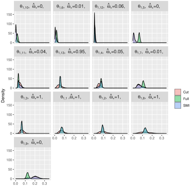
Appendix E Additional Results for Biased Means Example
In this section, we present the repeated sampling behavior of the cut, full and S-SMP in the simulation design presented in Section 3.2 of the main text and additional results on the behavior of the S-SMP for additional choices of . Please refer to the main text for full details of the simulation design.
Table 2 compares the behavior of the posterior mean for the three methods across different values of , and in the case where . Similar results for the case of are reported in Table 3. In each table we report the Bias of the posterior mean (Bias), the average posterior variance across the replications (Var) and the Monte Carlo coverage of a 95% posterior credible sets (Cov).
Regarding the results for and , we see that in both cases the the S-SMP attempts to trade-off bias in the full posterior for a significant reduction in variability. For both cases, the average cut posterior variance is about 0.01 across all values of , while the average S-SMP variance ranges from about to , which is significantly smaller than that of the cut posterior. Further, the bias exhibited by the S-SMP is generally much smaller than that exhibited by the full posterior, but is, by construction, larger than that exhibited by the cut posterior.
Recall that, as discussed in the remarks raised after the statement of Lemma 2 in the main text, under model misspecification only the cut posterior for can deliver credible sets that are also valid frequentist confidence sets. Analyzing the coverage of the posteriors across the two designs, we see that this is indeed the case, with only the cut posterior delivering accurate coverage. In comparison, in both cases, the full posterior has coverage that is zero or nearly zero once . The S-SMP fairs better than the full posterior, but can deliver unreliable coverage when . In contrast, as the dimension of increases to , the coverage of the S-SMP dramatically appreciates and in most cases is only slightly smaller than the nominal level for most values of . While not reported for the sake of brevity, extending these experiments to larger values of show that the coverage of the S-SMP improves as increases, so that when the coverage for the S-SMP is close to the nominal level across all values of used in the experiment.
Lastly, we demonstrate the impact on the accuracy of the S-SMP, as measured by expected squared error, as increases. To this end, we present the expected squared error of the cut, full and S-SMP for . We plot these results visually in Figure 9. Analyzing these results, we see that as increases, and for small, the S-SMP resembles the full posterior, but as increases the S-SMP more closely resemble the cut posterior. This is a consequence of the behavior of the pooling weight used in the S-SMP, which has an easier time shifting between the cut and full posterior when ; we refer to Section 4 in the main paper for a technical explanation of this phenomenon.
| Cut | Full | S-SMP | |||||||
|---|---|---|---|---|---|---|---|---|---|
| Bias | Var | Cov | Bias | Var | Cov | Bias | Var | Cov | |
| 0.1000 | -0.0081 | 0.0099 | 0.9400 | -0.0131 | 0.0001 | 0.7540 | -0.0098 | 0.0028 | 0.8190 |
| 0.1500 | -0.0080 | 0.0099 | 0.9410 | -0.0194 | 0.0001 | 0.5430 | -0.0121 | 0.0029 | 0.7040 |
| 0.2000 | -0.0082 | 0.0099 | 0.9410 | -0.0257 | 0.0001 | 0.3100 | -0.0143 | 0.0029 | 0.5800 |
| 0.2500 | -0.0080 | 0.0099 | 0.9430 | -0.0318 | 0.0001 | 0.1410 | -0.0161 | 0.0030 | 0.5050 |
| 0.3000 | -0.0082 | 0.0099 | 0.9400 | -0.0380 | 0.0001 | 0.0360 | -0.0182 | 0.0030 | 0.4560 |
| 0.3500 | -0.0080 | 0.0099 | 0.9430 | -0.0441 | 0.0001 | 0.0060 | -0.0198 | 0.0031 | 0.4520 |
| 0.4000 | -0.0081 | 0.0099 | 0.9400 | -0.0503 | 0.0001 | 0.0010 | -0.0218 | 0.0032 | 0.4610 |
| 0.4500 | -0.0081 | 0.0099 | 0.9420 | -0.0566 | 0.0001 | 0.0000 | -0.0234 | 0.0033 | 0.4720 |
| 0.5000 | -0.0082 | 0.0099 | 0.9420 | -0.0628 | 0.0001 | 0.0000 | -0.0248 | 0.0034 | 0.4810 |
| 0.5500 | -0.0081 | 0.0099 | 0.9430 | -0.0690 | 0.0001 | 0.0000 | -0.0261 | 0.0036 | 0.4950 |
| 0.6000 | -0.0082 | 0.0099 | 0.9420 | -0.0752 | 0.0001 | 0.0000 | -0.0276 | 0.0037 | 0.5010 |
| 0.6500 | -0.0081 | 0.0099 | 0.9400 | -0.0814 | 0.0001 | 0.0000 | -0.0289 | 0.0038 | 0.4950 |
| 0.7000 | -0.0081 | 0.0099 | 0.9430 | -0.0877 | 0.0001 | 0.0000 | -0.0302 | 0.0040 | 0.5010 |
| 0.7500 | -0.0081 | 0.0099 | 0.9410 | -0.0939 | 0.0001 | 0.0000 | -0.0314 | 0.0042 | 0.5170 |
| 0.8000 | -0.0079 | 0.0099 | 0.9420 | -0.1001 | 0.0001 | 0.0000 | -0.0321 | 0.0043 | 0.5440 |
| 0.8500 | -0.0081 | 0.0099 | 0.9410 | -0.1065 | 0.0001 | 0.0000 | -0.0332 | 0.0045 | 0.5580 |
| 0.9000 | -0.0082 | 0.0099 | 0.9430 | -0.1126 | 0.0001 | 0.0000 | -0.0340 | 0.0047 | 0.5790 |
| Cut | Full | S-SMP | |||||||
|---|---|---|---|---|---|---|---|---|---|
| Delta | Bias | Var | Cov | Bias | Var | Cov | Bias | Var | Cov |
| 0.1000 | -0.0074 | 0.0099 | 0.9550 | -0.0128 | 0.0005 | 0.9960 | -0.0107 | 0.0039 | 0.9800 |
| 0.1500 | -0.0075 | 0.0099 | 0.9530 | -0.0186 | 0.0005 | 0.9900 | -0.0135 | 0.0039 | 0.9790 |
| 0.2000 | -0.0075 | 0.0099 | 0.9540 | -0.0247 | 0.0005 | 0.9640 | -0.0162 | 0.0040 | 0.9770 |
| 0.2500 | -0.0073 | 0.0099 | 0.9540 | -0.0306 | 0.0005 | 0.8840 | -0.0185 | 0.0041 | 0.9560 |
| 0.3000 | -0.0075 | 0.0099 | 0.9530 | -0.0366 | 0.0005 | 0.7440 | -0.0213 | 0.0042 | 0.9220 |
| 0.3500 | -0.0075 | 0.0099 | 0.9570 | -0.0426 | 0.0005 | 0.5120 | -0.0235 | 0.0043 | 0.8750 |
| 0.4000 | -0.0074 | 0.0099 | 0.9540 | -0.0486 | 0.0005 | 0.2570 | -0.0256 | 0.0045 | 0.8360 |
| 0.4500 | -0.0073 | 0.0099 | 0.9550 | -0.0546 | 0.0004 | 0.1060 | -0.0275 | 0.0047 | 0.8130 |
| 0.5000 | -0.0074 | 0.0099 | 0.9550 | -0.0605 | 0.0004 | 0.0270 | -0.0293 | 0.0049 | 0.8150 |
| 0.5500 | -0.0074 | 0.0099 | 0.9550 | -0.0665 | 0.0004 | 0.0060 | -0.0306 | 0.0051 | 0.8290 |
| 0.6000 | -0.0074 | 0.0099 | 0.9550 | -0.0726 | 0.0004 | 0.0000 | -0.0318 | 0.0053 | 0.8400 |
| 0.6500 | -0.0073 | 0.0099 | 0.9560 | -0.0787 | 0.0004 | 0.0000 | -0.0326 | 0.0055 | 0.8570 |
| 0.7000 | -0.0074 | 0.0099 | 0.9560 | -0.0848 | 0.0004 | 0.0000 | -0.0335 | 0.0058 | 0.8640 |
| 0.7500 | -0.0073 | 0.0099 | 0.9530 | -0.0908 | 0.0004 | 0.0000 | -0.0338 | 0.0060 | 0.8790 |
| 0.8000 | -0.0075 | 0.0099 | 0.9550 | -0.0970 | 0.0004 | 0.0000 | -0.0342 | 0.0062 | 0.8830 |
| 0.8500 | -0.0074 | 0.0099 | 0.9560 | -0.1031 | 0.0004 | 0.0000 | -0.0343 | 0.0065 | 0.8980 |
| 0.9000 | -0.0074 | 0.0099 | 0.9550 | -0.1093 | 0.0003 | 0.0000 | -0.0344 | 0.0067 | 0.8990 |
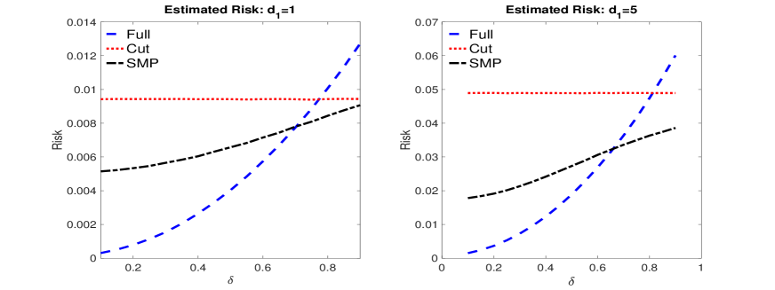
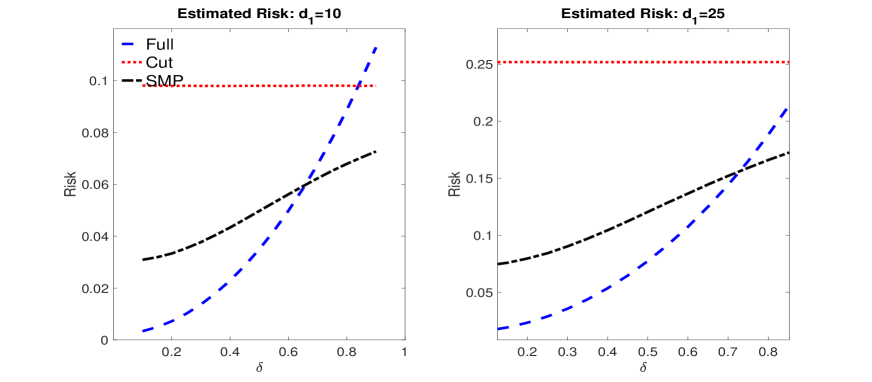
References
- Bennett and Wakefield [2001] Bennett, J. and J. Wakefield (2001). Errors-in-variables in joint population pharmacokinetic/pharmacodynamic modeling. Biometrics 57(3), 803–812.
- Bissiri et al. [2016] Bissiri, P. G., C. C. Holmes, and S. G. Walker (2016). A general framework for updating belief distributions. Journal of the Royal Statistical Society. Series B, Statistical methodology 78(5), 1103.
- Blangiardo et al. [2011] Blangiardo, M., A. Hansell, and S. Richardson (2011). A Bayesian model of time activity data to investigate health effect of air pollution in time series studies. Atmospheric Environment 45(2), 379–386.
- Carmona and Nicholls [2020] Carmona, C. and G. Nicholls (2020). Semi-modular inference: enhanced learning in multi-modular models by tempering the influence of components. In International Conference on Artificial Intelligence and Statistics, pp. 4226–4235. PMLR.
- Carmona and Nicholls [2022] Carmona, C. and G. Nicholls (2022). Scalable semi-modular inference with variational meta-posteriors. arXiv:2204.00296.
- Carpenter et al. [2017] Carpenter, B., A. Gelman, M. D. Hoffman, D. Lee, B. Goodrich, M. Betancourt, M. Brubaker, J. Guo, P. Li, and A. Riddell (2017, January). Stan: A Probabilistic Programming Language. Journal of Statistical Software 76(1), 1–32. Number: 1.
- Castillo [2014] Castillo, I. (2014). On Bayesian supremum norm contraction rates. Annals of Statistics.
- Chakraborty et al. [2022] Chakraborty, A., D. J. Nott, C. Drovandi, D. T. Frazier, and S. A. Sisson (2022). Modularized Bayesian analyses and cutting feedback in likelihood-free inference. Statistics and Computing (To appear).
- Claeskens and Hjort [2003] Claeskens, G. and N. L. Hjort (2003). The focused information criterion. Journal of the American Statistical Association 98(464), 900–916.
- Davidson [1994] Davidson, J. (1994). Stochastic limit theory: An introduction for econometricians. OUP Oxford.
- Frazier and Nott [2024] Frazier, D. T. and D. J. Nott (2024). Cutting feedback and modularized analyses in generalized Bayesian inference. Bayesian Analysis 1(1), 1–29.
- Gneiting and Raftery [2007] Gneiting, T. and A. E. Raftery (2007). Strictly proper scoring rules, prediction, and estimation. Journal of the American statistical Association 102(477), 359–378.
- Green and Strawderman [1991] Green, E. J. and W. E. Strawderman (1991). A James-Stein type estimator for combining unbiased and possibly biased estimators. Journal of the American Statistical Association 86(416), 1001–1006.
- Grünwald and Van Ommen [2017] Grünwald, P. and T. Van Ommen (2017). Inconsistency of Bayesian inference for misspecified linear models, and a proposal for repairing it. Bayesian Analysis 12(4), 1069–1103.
- Hansen [2016] Hansen, B. E. (2016). Efficient shrinkage in parametric models. Journal of Econometrics 190(1), 115–132.
- Hjort and Claeskens [2003] Hjort, N. L. and G. Claeskens (2003). Frequentist model average estimators. Journal of the American Statistical Association 98(464), 879–899.
- Jacob et al. [2017] Jacob, P. E., L. M. Murray, C. C. Holmes, and C. P. Robert (2017). Better together? Statistical learning in models made of modules. arXiv preprint arXiv:1708.08719.
- Jacob et al. [2020] Jacob, P. E., J. O’Leary, and Y. F. Atchadé (2020). Unbiased Markov chain Monte Carlo methods with couplings. Journal of the Royal Statistical Society: Series B (Statistical Methodology) 82(3), 543–600.
- Judge and Mittelhammer [2004] Judge, G. G. and R. C. Mittelhammer (2004). A semiparametric basis for combining estimation problems under quadratic loss. Journal of the American Statistical Association 99(466), 479–487.
- Kim and White [2001] Kim, T.-H. and H. White (2001). James-Stein-type estimators in large samples with application to the least absolute deviations estimator. Journal of the American Statistical Association 96(454), 697–705.
- Kleijn and van der Vaart [2012] Kleijn, B. and A. van der Vaart (2012). The Bernstein-von-Mises theorem under misspecification. Electron. J. Statist. 6, 354–381.
- Lee and Lee [2018] Lee, K. and J. Lee (2018). Optimal Bayesian minimax rates for unconstrained large covariance matrices. Bayesian Analysis.
- Lehmann and Casella [2006] Lehmann, E. L. and G. Casella (2006). Theory of point estimation. Springer Science & Business Media.
- Liu et al. [2009] Liu, F., M. Bayarri, and J. Berger (2009). Modularization in Bayesian analysis, with emphasis on analysis of computer models. Bayesian Analysis 4(1), 119–150.
- Liu and Goudie [2022a] Liu, Y. and R. J. B. Goudie (2022a). A general framework for cutting feedback within modularized Bayesian inference. arXiv:2211.03274.
- Liu and Goudie [2022b] Liu, Y. and R. J. B. Goudie (2022b). Stochastic approximation cut algorithm for inference in modularized Bayesian models. Statistics and Computing 32(7).
- Liu and Goudie [2023] Liu, Y. and R. J. B. Goudie (2023). Generalized geographically weighted regression model within a modularized Bayesian framework. Bayesian Analysis (To appear).
- Lunn et al. [2009] Lunn, D., N. Best, D. Spiegelhalter, G. Graham, and B. Neuenschwander (2009). Combining MCMC with ‘sequential’ PKPD modelling. Journal of Pharmacokinetics and Pharmacodynamics 36, 19–38.
- Maucort-Boulch et al. [2008] Maucort-Boulch, D., S. Franceschi, and M. Plummer (2008). International correlation between human papillomavirus prevalence and cervical cancer incidence. Cancer Epidemiology and Prevention Biomarkers 17(3), 717–720.
- Miller [2021] Miller, J. W. (2021). Asymptotic normality, concentration, and coverage of generalized posteriors. Journal of Machine Learning Research 22(168), 1–53.
- Newey [1985] Newey, W. K. (1985). Maximum likelihood specification testing and conditional moment tests. Econometrica: Journal of the Econometric Society, 1047–1070.
- Nicholls et al. [2022] Nicholls, G. K., J. E. Lee, C.-H. Wu, and C. U. Carmona (2022). Valid belief updates for prequentially additive loss functions arising in semi-modular inference. arXiv preprint arXiv:2201.09706.
- Plummer [2015] Plummer, M. (2015). Cuts in Bayesian graphical models. Statistics and Computing 25(1), 37–43.
- Pompe and Jacob [2021] Pompe, E. and P. E. Jacob (2021). Asymptotics of cut distributions and robust modular inference using posterior bootstrap. arXiv preprint arXiv:2110.11149.
- Rieder [2012] Rieder, H. (2012). Robust Asymptotic Statistics: Volume I. Springer Science & Business Media.
- Rousseau [1997] Rousseau, J. (1997). Asymptotic bayes risks for a general class of losses. Statistics & probability letters 35(2), 115–121.
- Shen and Wasserman [2001] Shen, X. and L. Wasserman (2001). Rates of convergence of posterior distributions. The Annals of Statistics 29(3), 687–714.
- Stone [1961] Stone, M. (1961). The opinion pool. The Annals of Mathematical Statistics, 1339–1342.
- Styring et al. [2017] Styring, A., M. Charles, F. Fantone, M. Hald, A. McMahon, R. Meadow, G. Nicholls, A. Patel, M. Pitre, A. Smith, A. Sołtysiak, G. Stein, J. Weber, H. Weiss, and A. Bogaard (2017). Isotope evidence for agricultural extensification reveals how the world’s first cities were fed. Nature Plants 3, 17076.
- Van der Vaart [2000] Van der Vaart, A. W. (2000). Asymptotic statistics, Volume 3. Cambridge University Press.
- Yu et al. [2023] Yu, X., D. J. Nott, and M. S. Smith (2023). Variational inference for cutting feedback in misspecified models. Statistical Science 38(3), 490–509.