Precision, Stability, and Generalization: A Comprehensive Assessment of RNNs learnability capability for Classifying Counter and Dyck Languages
Abstract
This study investigates the learnability of Recurrent Neural Networks (RNNs) in classifying structured formal languages, focusing on counter and Dyck languages. Traditionally, both first-order (LSTM) and second-order (O2RNN) RNNs have been considered effective for such tasks, primarily based on their theoretical expressiveness within the Chomsky hierarchy. However, our research challenges this notion by demonstrating that RNNs primarily operate as state machines, where their linguistic capabilities are heavily influenced by the precision of their embeddings and the strategies used for sampling negative examples. Our experiments revealed that performance declines significantly as the structural similarity between positive and negative examples increases. Remarkably, even a basic single-layer classifier using RNN embeddings performed better than chance. To evaluate generalization, we trained models on strings up to a length of 40 and tested them on strings from lengths 41 to 500, using 10 unique seeds to ensure statistical robustness. Stability comparisons between LSTM and O2RNN models showed that O2RNNs generally offer greater stability across various scenarios. We further explore the impact of different initialization strategies revealing that our hypothesis is consistent with various RNNs. Overall, this research questions established beliefs about RNNs’ computational capabilities, highlighting the importance of data structure and sampling techniques in assessing neural networks’ potential for language classification tasks. It emphasizes that stronger constraints on expressivity are crucial for understanding true learnability, as mere expressivity does not capture the essence of learning.
1 Introduction
Recurrent neural networks (RNNs) are experiencing a resurgence, spurring significant research aimed at establishing theoretical bounds on their expressivity. As natural neural analogs to state machines described by the Chomsky hierarchy, RNNs offer a robust framework for examining learnability, stability, and generalization—core aspects for advancing the development of memory-augmented models.
While conventional RNN architectures typically approximate finite state automata, LSTMs have shown the capacity to learn and generalize non-regular grammars, including counter languages and Dyck languages. These non-regular grammars demand a state machine enhanced with a memory component, and LSTM cell states have been demonstrated to possess sufficient expressivity to mimic dynamic counters. However, understanding whether these dynamics are stable and reliably learnable is crucial, particularly as the stability of learned fixed points directly impacts the generalization and reliability of these networks.
In this work, we extend the investigation into the expressiveness of RNNs by focusing on the empirical evidence for learnability and generalization in complex languages, with specific attention to Dyck and counter languages. Our analysis reveals the following key insights:
-
1.
The counter dynamics learned by LSTM cell states are prone to collapse, leading to unstable behavior.
-
2.
When positive and negative samples are not topologically proximal, the classifier can obscure the collapse of counter dynamics, creating an illusion of generalization.
-
3.
The initial weight distribution has little effect on the eventual collapse of counter dynamics, suggesting inherent instability.
-
4.
Second-order RNNs, although stable in approximating fixed states, lack the mechanism required for counting, underscoring the limitations of their expressivity.
Our analysis builds upon results from [1] regarding the behavior of the sigmoid activation function, extending this understanding to the fixed points of the tanh function used in LSTM cell and hidden state updates. Drawing from parallels noted by [2] between LSTMs and counter machines, we show that while LSTM cell states exhibit the expressivity needed for counting, this capability is not reliably captured in the hidden state. As a result, when the difference between successive hidden states falls below the precision threshold of the decoder, the classifier can no longer accurately represent the counter, leading to generalization failure. Additionally, we explore how input and forget gates within the LSTM clear the counter dynamics as state changes accumulate, resulting in an eventual collapse of dynamic behavior.
Further, we extend our exploration to analyze the learnability of classification layers when the encoding RNN is initialized randomly and not trained. This setup allows us to assess the extent of instability induced by the collapse of counter dynamics in the LSTM cell state and the role of numeric precision in the hidden state that supports the classification layer’s performance.
It is crucial to recognize that most prior studies demonstrating the learnability of RNNs on counter languages such as , , and have overlooked the significance of topological distance between positive and negative samples. Such sampling considerations are vital for a thorough understanding of RNN trainability. To address this gap, we incorporate three sampling strategies with varying levels of topological proximity between positive and negative samples, thereby challenging the RNNs to genuinely learn the counting mechanism.
By focusing on stability and fixed-point dynamics, our work offers a plausible lens through which the learnability of complex grammars in recurrent architectures can be better understood. We argue that stability, as characterized by the persistence of fixed points, is a critical factor in determining whether these models can generalize and reliably encode non-regular languages, shedding light on the inherent limitations and potentials of RNNs in such tasks.
2 Related Work
The relationship between Recurrent Neural Networks (RNNs), automata theory, and formal methods has been a focal point in understanding the computational power and limitations of neural architectures. Early studies have shown that RNNs can approximate the behavior of various automata and formal language classes, providing insights into their expressivity and learnability. [3] was one of the first to demonstrate that RNNs are capable of learning finite automata. They extracted finite state machines from trained RNNs, showing that the learned rules could be represented as deterministic automata. This foundational work laid the groundwork for subsequent studies on how RNNs encode and process state-based structures. Expanding on this, [4] showed that second-order recurrent networks, which include multiplicative interactions between inputs and hidden states, are superior state approximators compared to standard first-order RNNs. This enhancement in state representation significantly improved the networks’ ability to learn and represent complex sequences.
The analysis of RNNs’ functional capacity continued with [1, 5], who investigated the discriminant functions underlying first-order and second-order RNNs. Their results provided a deeper understanding of how these architectures utilize hidden state dynamics to implement decision boundaries and process temporal patterns. Meanwhile, the theoretical limits of RNNs were formalized by [6], who proved that RNNs are Turing Complete when equipped with infinite precision. This result implies that RNNs, in principle, can simulate any computable function, positioning them as universal function approximators.
Building on these foundational insights, recent research has aimed to identify the practical scenarios under which RNNs can achieve such theoretical expressiveness. [5] extended Turing completeness results to a second-order RNN, demonstrating that it can achieve Turing completeness in bounded time, making it relevant for real-world applications where resources are constrained. This shift towards practical expressivity has opened new avenues for applying RNNs to complex language tasks. Moving towards specific language modeling tasks, [7] explored how Long Short-Term Memory (LSTM) networks can learn context-free and context-sensitive grammars, such as and . Their results showed that LSTMs could successfully learn these patterns, albeit with limitations in scaling to larger sequence lengths. Extending these findings, [2] established a formal hierarchy categorizing RNN variants based on their expressivity, placing LSTMs in a higher class due to their ability to simulate counter machines. This formal classification aligns with the observation that LSTMs can implement complex counting and state-tracking mechanisms, making them suitable for tasks involving nested dependencies. Further investigations into RNNs’ capacity to recognize complex languages have revealed both strengths and limitations. [8] analyzed the ability of LSTMs to learn the Dyck-1 language, which models balanced parentheses, and found that while a single LSTM neuron could learn Dyck-1, it failed to generalize to Dyck-2, a more complex language with nested dependencies. Their follow-up work [9] studied generalization on , , and grammars, showing that performance varied significantly with sequence length sampling strategies. These findings highlight that while RNNs can theoretically represent these languages, practical training limitations impede their learnability.
Beyond traditional RNNs, the role of specific activation functions in enhancing expressivity has also been studied. [10] showed that RNNs with ReLU activations are strictly more powerful than those using standard sigmoid or tanh activations when it comes to counting tasks. This observation suggests that architectural modifications can significantly alter the network’s functional capacity. In a similar vein, [11] proposed neural network pushdown automata and neural network Turing machines, establishing a theoretical framework for integrating stacks into neural architectures, thereby enabling them to simulate complex computational models like pushdown automata and Turing machines. On the stability and generalization front, [12] compared the stability of states learned by first-order and second-order RNNs when trained on Tomita and Dyck grammars. Their results indicate that second-order RNNs are better suited for maintaining stable state representations across different grammatical tasks, which is critical for ensuring that the learned model captures the true structure of the language. Their work also explored methods for extracting deterministic finite automata (DFA) from trained networks, evaluating the effectiveness of extraction techniques like those proposed by [13] and [14]. This line of research is pivotal in understanding how well trained RNNs can be interpreted and how their internal state representations correspond to formal structures.
In terms of language generation and hierarchical structure learning, [15] demonstrated that LSTMs, when trained as language generators, can learn Dyck- languages, which involve hierarchical and nested dependencies, drawing parallels between these formal languages and syntactic structures in natural languages. Finally, several studies have shown that the choice of objective functions and learning algorithms significantly affects RNNs’ ability to stably learn complex grammars. For instance, [16] and [17] demonstrated that specialized loss functions, such as minimum description length, lead to more stable convergence and better generalization on formal language tasks. In light of the diverse findings from the aforementioned studies, our work systematically analyzes the divergence between the theoretical expressivity of RNNs and their empirical generalization capabilities through the lens of fixed-point theory. Specifically, we investigate how different RNN architectures capture and maintain stable state representations when learning complex grammars, focusing on the role of numerical precision, learning dynamics, and model stability. By leveraging theoretical results on fixed points and state stability, we provide a unified framework to evaluate the strengths and limitations of various RNN architectures.
The remainder of the paper is organized as follows: In Section 3, we present theoretical results on the fixed points of discriminant functions, providing foundational insights into the stability properties of RNNs. Section 4 extends these results by introducing a formal framework for analyzing RNNs as counter machines, highlighting how cell update mechanisms contribute to language recognition. Section 5 focuses on the impact of numerical precision on learning dynamics and convergence. Section 6 describes the experimental setup and empirical evaluation on complex formal languages, including Dyck and Tomita grammars. Finally, Section 7 discusses the broader implications of our findings and suggests future research directions.
3 Fixed Points of Discriminant Functions
In this section we focus on two prominent discriminant functions: sigmoid and tanh, both of which are extensively utilized in widely-adopted RNN cells such as LSTM and O2RNN.
Theorem 3.1.
BROUWER’S FIXED POINT THEOREM [18]: For any continuous mapping , where Z is a compact, non-empty convex set, s.t.
Corollary 3.1.1.
Let be a continuous, monotonic function with a non-empty, bounded, and convex co-domain . Then has at least one fixed point, i.e., there exists some such that .
Proof.
Since is a non-empty, bounded, and convex set, let the co-domain of be denoted as for some with . Consider the identity function , which is continuous on . The fixed points of correspond to the points of intersection between and , i.e., the solutions to the equation .
Next, observe the behavior of outside its co-domain :
-
•
For any , we have (since is monotonic), implying that .
-
•
For any , we have , implying that .
By the Intermediate Value Theorem, if for some and for some , then there must exist a point such that .
Thus, the function has at least one fixed point in the interval .
∎
Corollary 3.1.2.
A parameterized sigmoid function of the form , where , has at least one fixed point, i.e., there exists some such that .
Proof.
Consider the function . We want to show that has at least one fixed point. A fixed point is a value such that .
First, observe that the sigmoid function is continuous and strictly increasing for all . The co-domain of is the interval , i.e., for all . We now consider the continuous identity function , which intersects the line .
Next, let us analyze the behavior of as and :
-
•
As , we have , which implies . Therefore, as .
-
•
As , we have , which implies . Therefore, as .
Since is a continuous function on and changes sign (from positive to negative) as varies from to , by the Intermediate Value Theorem, there must exist some such that:
Hence, has at least one fixed point.
∎
Corollary 3.1.3.
A parameterized function of the form , where , has at least one fixed point, i.e., there exists some such that .
Proof.
Consider the function . We want to show that has at least one fixed point. A fixed point is a value such that .
Step 1: Properties of the Function The hyperbolic tangent function, , is a continuous and strictly increasing function for all . For any real value , the function is bounded and satisfies . Thus, the co-domain of is also bounded within , i.e., for all .
Furthermore, since is strictly increasing, the function is also strictly increasing in . This implies that is one-to-one and continuous over .
Step 2: Analysis of Consider the function:
We want to show that has at least one solution, i.e., there exists some such that . To analyze the existence of such a , let us examine the behavior of as :
- As : We have . Thus, . Therefore:
- As : We have . Thus, . Therefore:
Since is continuous on and changes sign from positive (as ) to negative (as ), by the Intermediate Value Theorem, there must exist some such that:
This implies that , i.e., has at least one fixed point.
∎
Prior [1] have shown that parameterized sigmoid function has three fixed points for a given and for some and . Further they showed sigmoid has two stable fixed point. In this work we go beyond sigmoid and show that TanH also has three fixed points
Theorem 3.2.
A parameterized function has three fixed points for a given and for some and .
Proof.
We start by defining a fixed point of the function . A fixed point satisfies the equation:
Let us define a new function to analyze the fixed points:
The fixed points of are the solutions to the equation . We will analyze in detail to determine the number of solutions.
Step 1: Properties of
The function is continuous and differentiable. We start by computing its derivative:
where is the hyperbolic secant function. The value of satisfies . Thus:
Step 2: Critical Points of
The critical points occur when :
Since , the above equation has a real solution if and only if:
For , there are exactly two critical points, and , such that .
Step 3: Behavior of as
As , for . Thus, . Hence:
Therefore, as .
As , for . Thus, . Hence:
Therefore, as .
Step 4: Intermediate Value Theorem
The intermediate value theorem tells us that since is continuous and changes sign from to , it must have at least one root. Thus, there is at least one fixed point for .
Step 5: Conditions for Three Fixed Points
We want to show that for specific values of and , the function has exactly three roots. To do so, we analyze in detail around its critical points.
1. Critical Points Analysis:
Recall that the critical points of are given by:
Let . Then the critical points and satisfy:
Solving for , we get:
Converting back to :
2. Local Minima and Maxima Analysis:
At these critical points, the second derivative determines whether has a local minimum or maximum:
Analyzing and , we can show that corresponds to a local minimum and corresponds to a local maximum (or vice-versa depending on ).
3. Behavior of in the Range :
For and , changes sign three times, indicating three distinct zeros.
Thus, for and , the function has exactly three fixed points.
∎
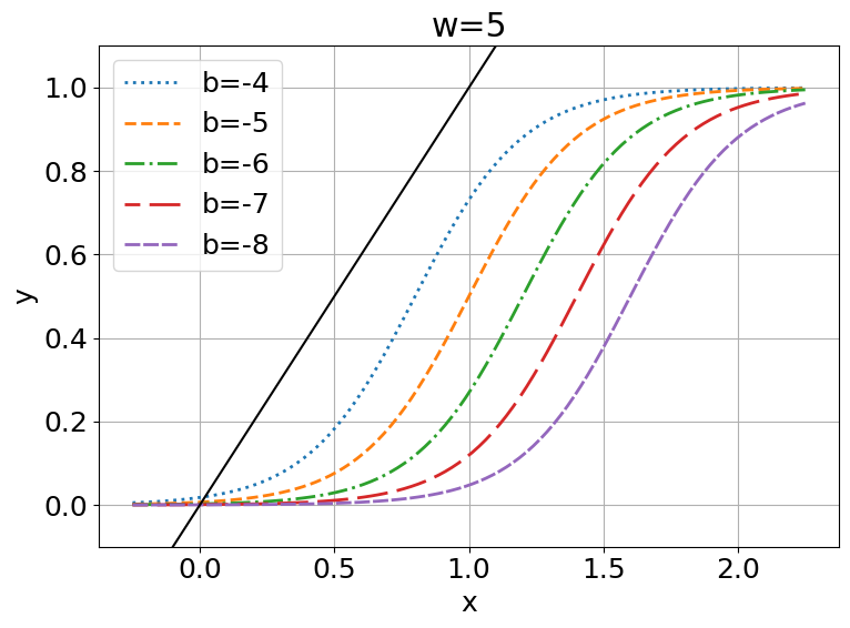
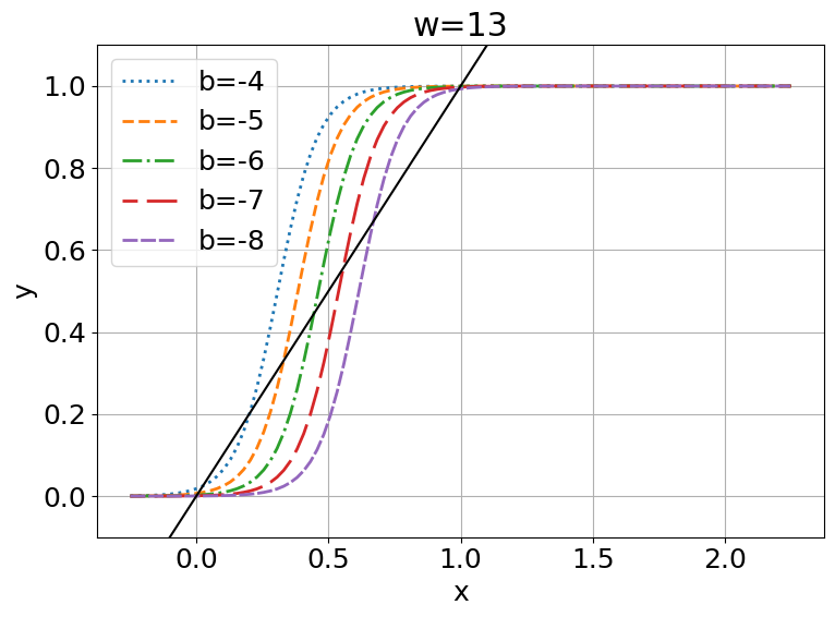
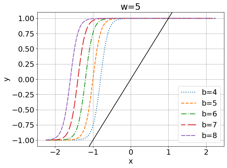
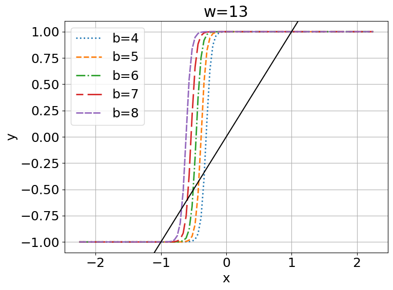
This can be visualized in Figure 1(c, d). Let , then we can observe that meets three times for , while it only meets once for . Since is also a monotonic function, and and will have a monotonic inverse relationship, for all , has fixed points.
Next we show Tanh has out of three fixed point, two stable fixed points stable
Theorem 3.3.
If a parameterized function has three fixed points such that , then and are stable fixed points.
Proof.
Let us start by defining a fixed point of the function . A point is a fixed point if:
We are given that there are three fixed points such that:
Step 1: Stability Criterion for Fixed Points A fixed point is considered stable if the magnitude of the derivative of at is less than 1, i.e.,
Conversely, a fixed point is unstable if:
Step 2: Derivative of the Function We compute the derivative of :
Recall that the derivative of the hyperbolic tangent function is:
where . Using the chain rule, we obtain:
Thus, at a fixed point , the derivative is:
Step 3: Stability Analysis at Each Fixed Point We will now analyze the derivative at each of the three fixed points to determine their stability.
1. Middle Fixed Point :
Since is the middle fixed point, the function has a steep slope at . Intuitively, the slope of around the origin (and for values near zero) is steep, making . Thus, is an unstable fixed point.
2. Leftmost Fixed Point :
Consider the derivative at the leftmost fixed point :
Since is smaller in magnitude compared to , the value of is close to 1 but slightly less, and thus:
This implies that the fixed point is stable.
3. Rightmost Fixed Point :
Similarly, for the rightmost fixed point :
Since is greater than , the value of is also close to 1 but less than at , leading to:
This means that the fixed point is stable.
Thus we have shown that for the three fixed points , , and of the function :
- is an unstable fixed point because . - and are stable fixed points because and .
Thus, the theorem is proven. ∎
We can make the following observations about the fixed points of sigmoid and tanh functions:
-
•
If one fixed point exists, then it is a stable fixed point
-
•
If two fixed point exists, then one fixed point is stable and other is unstable.
-
•
If three fixed point exists, then two fixed points are stable and one is unstable.
More details regarding these observations can be found in the Appendix.
4 Counter Machines
Counter machines [19] are abstract machines composed of finite state automata controlling one or more counters. A counter can either increment (), decrement ( if ), clear (), do nothing (). A counter machine can be formally defined as:
Definition 4.1.
A counter machine (CM) is a 7-tuple where
-
•
is a finite alphabet
-
•
is a set of states with as initial state
-
•
is a set of accepting states.
-
•
checks the state of the counter and returns if counter is zero else returns
-
•
is the counter update function defined as:
(1) -
•
is the state transition function defined as:
(2)
Acceptance of a string in a counter machine can be assessed by either the final state is in or the counter reaches at the end of the input.
5 Learning to accept with LSTM
LSTM [20] is a gated RNN cell. The LSTM state is a tuple where is popularly known as hidden state and is known as cell state.
| (3) | ||||
| (4) | ||||
| (5) | ||||
| (6) | ||||
| (7) | ||||
| (8) |
A typical binary classification network with LSTM cell is composed of two parts:
-
1.
The enocoder recurrent network
(9) -
2.
A classification layer, usually a single perceptron layer followed by a sigmoid
(10) In case of multiclass classification, is replaced by softmax function.
Following the construction of [2] we can draw parallels between the workings of counter machine and LSTM cell. Here decides wheather to execute , while are decided by . To execute both and needs to be .
Also the cell state and hidden state of LSTM have tanh as discriminant function. In the case of , a continuous stream of is followed by an equal number of , which creates an iterative execution of LSTM cell, making the output of discriminant functions closer to their fixed points. For maximum learnability, we can assume . Thus maximum final state values for will be:
| (11) | ||||
| (12) |
From the above equations we can see that, while cell state is unbounded, hidden state is bounded in range . In our experiments we see that hidden state saturates to boundary values faster than is required to maintain the count. Formally, for some fairly moderate and we can reach a point where , where is the precision of the classification layer.
Saturation of hidden state is desired from the perspective of consistent calculation of counter updates. In the LSTM cell, saturated hidden state means more stable gates which in turn leads to consistent cell state. However from the perspective of the classification layer, a saturated hidden state does not offer much information for a robust classification.
6 Precision of Neural Network
Numerical precision plays an important role in the partition of feature space by the classifier network, especially when the final hidden state from RNN either collapses towards or saturates asymptotically to the boundary values.
Theorem 6.1.
Given a neural network layer with an input vector , a weight matrix , a bias vector , and a sigmoid activation function , the output of the layer is defined by . The capacity of this layer to encode information is influenced by both the precision of the floating-point representation and the dynamical properties of the sigmoid function.
Let be the machine epsilon, which represents the difference between 1 and the least value greater than 1 that is representable in the floating-point system used by the network. Assume the elements of and are drawn from a Gaussian distribution and are fixed post-initialization.
Then, the following bounds hold for the output of the network layer:
-
1.
The granularity of the output is limited by , such that for any element in and corresponding weight in , the difference in the layer’s output due to a change in or less than may be imperceptible.
-
2.
For , the sigmoid function saturates to 1 as and to 0 as . The saturation points occur approximately at and , respectively.
-
3.
The precision of the network’s output is governed by the stable fixed points of the sigmoid function, which occur when stabilizes at values near 0 or 1. If the dynamics of the network converge to one or more stable fixed points, the effective precision is reduced because minor variations in the input will not significantly alter the output.
-
4.
When three fixed points exist for the sigmoid function—two stable and one unstable—information encoding can become confined to the stable fixed points. This behavior causes the network to collapse to a discrete set of values, reducing its effective resolution.
-
5.
Therefore, the maximum discrimination in the output is not only limited by but also by the attraction of the stable fixed points. The effective precision is bounded by both and the dynamics that collapse the output towards these stable points.
The detailed proof can be found in the appendix.
Theorem 6.2.
Consider a recurrent neural network (RNN) with fixed weights and the hidden state update rule given by:
where , , , and represents the input symbol. Given a bounded sequence length , the RNN can encode sequences of the form by exploiting state dynamics that converge to distinct, stable fixed points in the hidden state space for each symbol. The expressivity of the RNN, equivalent to a deterministic finite automaton (DFA), enables the encoding of such grammars purely through state dynamics.
The detailed proof can be found in appendix
Theorem 6.3.
Given an RNN with fixed random weights and trainable sigmoid layer has sufficient capacity to encode complex grammars. Despite the randomness of the recurrent layer, the network can still classify sequences of the form by leveraging the distinct distributions of the hidden states induced by the input symbols. The classification layer learns to map the hidden states to the correct sequence class, even for bounded sequence lengths .
Proof.
The proof proceeds in three steps: (1) analyzing the hidden state dynamics in the presence of random fixed weights, (2) demonstrating that distinct classes (e.g., ) can still be linearly separable based on the hidden states, and (3) showing that the classification layer can be trained to distinguish these hidden state patterns.
1. Hidden State Dynamics with Fixed Random Weights:
Consider an RNN with hidden state updated as:
where and are randomly initialized and fixed. The hidden state dynamics in this case are governed by the random projections imposed by and .
Although the weights are random, the hidden state still carries information about the input sequence. Specifically, different sequences (e.g., , , and ) induce distinct trajectories in the hidden state space. These trajectories are not arbitrary but depend on the input symbols, even under random weights.
2. Distinguishability of Hidden States for Different Sequence Classes:
Despite the randomness of the weights, the hidden state distributions for different sequences remain distinguishable. For example: - The hidden states after processing tend to cluster in a specific region of the state space, forming a characteristic distribution. - Similarly, the hidden states after processing and will occupy different regions.
These clusters may not correspond to single fixed points as in the trained RNN case, but they still form distinct, linearly separable patterns in the high-dimensional space.
3. Training the Classification Layer:
The classification layer is a fully connected layer that maps the final hidden state to the output class (e.g., ”class 1” for ). The classification layer is trained using a supervised learning approach, typically minimizing a cross-entropy loss.
Because the hidden states exhibit distinct distributions for different sequences, the classification layer can learn to separate these distributions. In high-dimensional spaces, even random projections (as induced by the random recurrent weights) create enough separation for the classification layer to distinguish between different classes.
Thus even with random fixed weights, the hidden state dynamics create distinguishable patterns for different input sequences. The classification layer, which is the only trained component, leverages these patterns to correctly classify sequences like . This demonstrates that the RNN’s expressivity remains sufficient for the classification task, despite the randomness in the recurrent layer.
∎
7 Experiment Setup
|
|
|
|
|
|||||||||||||||
|---|---|---|---|---|---|---|---|---|---|---|---|---|---|---|---|---|---|---|---|
| grammars | sdim | max | mean±std | max | mean±std | max | mean±std | max | mean±std | ||||||||||
| Dyck- | 2 | 85.95 | 82.88 ± 2.54 | 73.89 | 72.3 ± 1.28 | 83.38 | 80.57 ± 2.37 | 63.88 | 63.85 ± 0.02 | ||||||||||
| Dyck- | 4 | 98.65 | 87.35 ± 8.3 | 72.99 | 70.05 ± 3.35 | 86.85 | 82.57 ± 2.11 | 63.67 | 60.75 ± 2.41 | ||||||||||
| Dyck- | 8 | 99.2 | 86.57 ± 8.01 | 71.93 | 69.58 ± 3.71 | 99.11 | 94.55 ± 0.85 | 63.71 | 59.88 ± 2.44 | ||||||||||
| Dyck- | 12 | 97.45 | 87.34 ± 8.85 | 72.27 | 68.64 ± 2.24 | 99.54 | 98.4 ± 1.42 | 62.74 | 60.33 ± 1.79 | ||||||||||
| 6 | 98.13 | 90.17 ± 15.30 | 81.09 | 78.60 ± 1.54 | 97.86 | 97.27 ± 0.35 | 69.71 | 69.66 ± 0.03 | |||||||||||
| 8 | 98.33 | 90.45 ± 14.22 | 80.95 | 79.59 ± 0.97 | 97.24 | 96.11 ± 2.43 | 71.8 | 71.74 ± 0.03 | |||||||||||
| 8 | 99.83 | 98.05 ± 4.65 | 70.83 | 69.69 ± 0.74 | 99.76 | 99.58 ± 0.19 | 58.7 | 58.08 ± 0.48 | |||||||||||
| 8 | 99.93 | 99.64 ± 0.56 | 73.25 | 70.59 ±1.18 | 99.43 | 99.13 ± 0.38 | 58.67 | 56.95 ± 2.58 | |||||||||||
Models
We evaluate the performance of two types of Recurrent Neural Networks (RNNs): Long Short-Term Memory (LSTM) networks [20] and Second-Order Recurrent Neural Networks (O2RNNs) [21]. The LSTM is considered a first-order RNN since its weight tensors are second-order matrices, whereas the O2RNN utilizes third-order weight tensors for state transitions, making it a second-order RNN. The state update for the O2RNN is defined as follows:
where is a third-order tensor that models the interactions between the input vector and the previous hidden state , and is the bias term. All models consist of a single recurrent layer followed by a sigmoid activation layer for binary classification, as defined in Equation 10.
Datasets
We conduct experiments on eight different formal languages, divided into two categories: Dyck languages and counter languages. The Dyck languages include Dyck-1, Dyck-2, Dyck-4, and Dyck-6, which vary in the complexity and depth of nested dependencies. The counter languages include , , , and . Each language requires the network to learn specific counting or hierarchical patterns, posing unique challenges for generalization.
The number of neurons used in the hidden state for each RNN configuration is summarized in Table 1. To ensure robustness and a fair comparison, all models were trained on sequences with lengths ranging from 1 to 40 and tested on sequences of lengths ranging from 41 to 500, thereby evaluating their generalization capability on longer and more complex sequences.
Training and Testing Methodology
Since the number of possible sequences grows exponentially with length (for a sequence of length , there are possible combinations), we sampled sequences using an inverse exponential distribution over length, ensuring a balanced representation of short and long strings during training. Each model was trained to predict whether a given sequence is a positive example (belongs to the target language) or a negative example (does not follow the grammatical rules of the language).
For all eight languages, positive examples are inherently sparse in the overall sample space. This sparsity makes the generation of negative samples crucial to ensure a challenging and informative training set. We generated three different datasets, each using a distinct strategy for sampling negative examples:
-
1.
Hard 0 (Random Sampling): Negative samples were randomly generated from the sample space without any structural similarity to positive samples. This method creates a broad variety of negatives, but many of these are trivially distinguishable, providing limited learning value for more sophisticated models.
-
2.
Hard 1 (Edit Distance Sampling): Negative samples were constructed based on their string edit distance from positive examples. Specifically, for a sequence of length , we generated negative strings that have a maximum edit distance of . This approach ensures that negative samples are structurally similar to positive ones, making it challenging for the model to differentiate them based solely on surface-level patterns.
-
3.
Hard 2 (Topological Proximity Sampling): Negative samples were generated using topological proximity to positive strings, based on the structural rules of the language. For instance, in the counter language , a potential negative string could be , which maintains a similar overall structure but violates the language’s grammatical constraints. This method ensures that the negative samples are more nuanced, requiring the model to maintain precise state transitions and counters to correctly classify them.
Training Details For reproducibility and stability we train each model over seeds and report the mean, standard deviation, and maximum of accuracy over test set. We use stochastic gradient descent optimizer for a maximum of iterations. We employ a batch size of and a learning rate of . Validation is run very iterations and training is stopped if validation loss does not improve for consecutive iterations. All models use binary cross entropy loss as optimization function.
We use uniform random initialization (, where is the hidden size) for LSTM weights and normal initialization () for O2RNN for all experiments, except figure 4 which compares performance of LSTM and O2RNN on with the following initialization strategies:
-
1.
uniform initialization :
-
2.
orthogonal initialization : gain =
-
3.
sparse initialization : sparsity = , all non zero are sampled from
All the biases are initialized with a constant value of
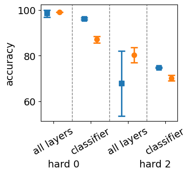
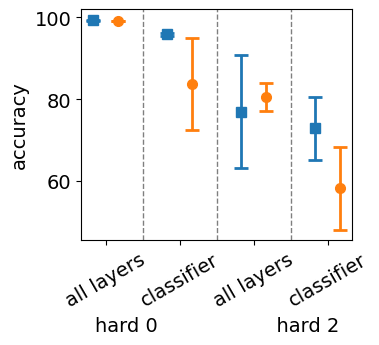
Tables 1 and 2 show results comparing models trained in two different ways : (1) all layers: all layers of the model are trained, and (2) classifier-only: weights of the RNN cells are frozen after random initialization and only classifier is trained.
We use Nvidia 2080ti GPUs to run our experiments with training times varying from under minutes for a simpler dataset like Dyck- on O2RNN, to over minutes for a counter language on LSTM. In total, we train models for our main results with over hours of cumulative GPU training times.
8 Results and Discussion
|
|
|
|
||||||||||||||
|---|---|---|---|---|---|---|---|---|---|---|---|---|---|---|---|---|---|
| grammar | neg set | max | mean ± std | max | mean ± std | max | mean ± std | max | mean ± std | ||||||||
| hard 0 | 99.92 | 99.28 ± 0.29 | 96.13 | 93.14 ± 2.53 | 99.61 | 99.27 ± 0.48 | 83.37 | 83.32 ± 0.03 | |||||||||
| hard 1 | 98.13 | 90.17 ± 15.30 | 81.09 | 78.60 ± 1.54 | 97.86 | 97.27 ± 0.35 | 69.71 | 69.66 ± 0.03 | |||||||||
| hard 2 | 87.49 | 74.35 ± 13.23 | 75.64 | 74.48 ± 0.73 | 86.42 | 82.10 ± 3.3 | 69.94 | 69.85 ± 0.07 | |||||||||
| hard 0 | 99.59 | 99.36 ± 0.19 | 98.1 | 95.94 ± 1.49 | 99.48 | 98.91 ± 1.17 | 87.53 | 87.5 ± 0.02 | |||||||||
| hard 1 | 98.33 | 90.45 ± 14.22 | 80.95 | 79.59 ± 0.97 | 97.24 | 96.11 ± 2.43 | 71.8 | 71.74 ± 0.03 | |||||||||
| hard 2 | 85.81 | 71.66 ± 12.21 | 75.33 | 74.47 ± 1.29 | 85.61 | 80.84 ± 3.68 | 70.72 | 70.66 ± 0.03 | |||||||||

gain =
sparsity =
Learnability of Dyck and Counter Languages
The results from Table 2 for negative set hard 0 confirm prior findings on the expressivity of LSTMs and RNNs on counter, context-free, and context-sensitive languages. A one-layer LSTM is theoretically capable of representing all classes of counter languages, indicating that its expressivity is sufficient to model non-regular grammars. However, the results for negative sets hard 1 and hard 2 indicate that this expressivity does not necessarily translate to practical learnability. The observed performance drop on these harder negative sets suggests that, despite the LSTM’s capacity to model such languages, its ability to generalize correctly under realistic training conditions is limited. This discrepancy between expressivity and learnability calls for a deeper understanding of how the network’s internal dynamics align with the objective function during training.
In particular, the sparsity of positive samples combined with naively sampled negative examples (as in hard 0) allows the classifier to partition the feature space even when the internal feature encodings are not well-structured. This may give an inflated impression of the LSTM’s practical learnability. Tables 1 and 2 compare fully trained models and classifier-only trained models, showing that the latter can achieve above-chance accuracy, even with minimal feature encoding. When negative samples are sampled closer to positive ones, as in hard 1 and hard 2, the classifier struggles to maintain robust partitions, highlighting that the underlying feature encodings are not sufficiently aligned with the grammar structure. Future work can leverage fixed-point theory and expressivity analysis to establish better learnability bounds, offering a more principled approach to bridge the gap between theoretical capacity and empirical generalization.
Stability of Feature Encoding in LSTM
The stability of LSTM feature encodings is heavily influenced by the precision of the network’s internal dynamics. Across 10 random seeds, the standard deviation of accuracy for fully trained LSTMs is significantly higher compared to classifier-only models, particularly for challenging sampling strategies. For example, a fully trained LSTM on shows a standard deviation of 15.30% compared to only 1.54% for the classifier-only network using hard 1 sampling. This difference is less pronounced for hard 0 (0.29%) but becomes more severe for hard 2 (13.23%), indicating that instability in the learned feature encodings increases as the negative examples become structurally closer to positive ones. This instability is due to the LSTM’s reliance on its cell state to encode dynamic counters, which may not align precisely with the hidden state used for classification. As a result, slight deviations in internal dynamics cause substantial fluctuations in performance, suggesting a lack of robust fixed-point behavior in the cell state.
Stability of Second-Order RNNs
In contrast, the O2RNN, which utilizes a third-order weight tensor, demonstrates more consistent performance across different training strategies and random seeds. In all configurations, the O2RNN exhibits a standard deviation of less than 3%, as shown in Tables 1 and 2. This stability is attributed to the higher-order interactions in the weight tensor, which drive the activation dynamics towards more stable fixed points. The convergence to these stable fixed points results in more robust internal state representations, making the O2RNN less sensitive to variations in training data and initialization. These findings are consistent with observations by [12] for regular and Dyck languages, suggesting that higher-order tensor interactions inherently stabilize the internal dynamics, improving the alignment between the learned state transitions and the theoretical expressive capacity.
Dynamic Counting and Fixed Points
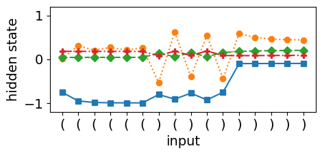
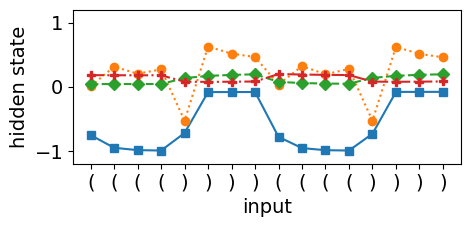
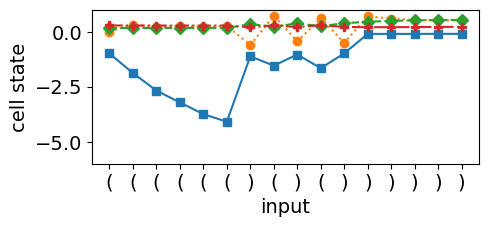
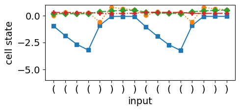
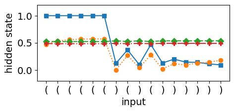
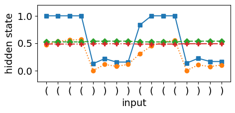
The LSTM’s ability to perform dynamic counting is closely tied to the stability of its cell state, which relies on the fixed points of the tanh activation function, as shown in Equation 11. Figures 2(c) and 2(d) provide evidence of dynamic counting when the LSTM encounters consecutive open brackets, as indicated by the solid blue curve that decreases monotonically. This behavior is in accordance with Equation 12, where the hidden state saturates to -1. However, when the network encounters a closing bracket, the cell state counter collapses, causing the hidden and cell states to start mirroring each other. This collapse occurs due to a mismatch between the counter dynamics and the LSTM’s training objective, which primarily optimizes for hidden state changes rather than directly influencing the cell state’s stability.
The root cause lies in the misalignment between the counter dynamics and the classification objective. Since the classification layer only uses the hidden state as input, any instability in the cell dynamics propagates through the hidden state, making it difficult for the network to maintain precise counter updates. In contrast, the O2RNN’s pure state approximation mechanism, as illustrated in Figure 3, shows smoother transitions and stable dynamics, indicating that the network’s internal states are better aligned with its expressivity requirements.
Effect of Initialization on Fixed-Point Stability
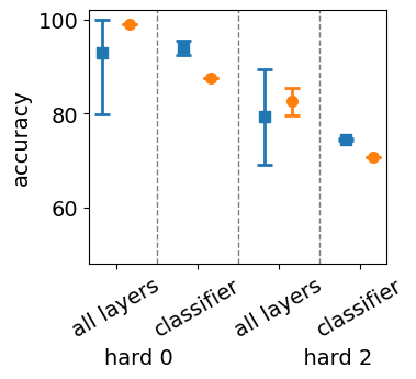
The choice of initialization strategy significantly influences the stability of fixed points in RNNs. Figure 4 shows that the performance of both LSTMs and O2RNNs declines from hard 0 to hard 1 for all initialization strategies. However, we observe that the O2RNN is particularly sensitive to sparse initialization, while being more stable for the other two initialization methods. This sensitivity reflects the network’s reliance on precise weight configurations to drive its activation dynamics towards stable fixed points. In contrast, the LSTM’s performance is relatively invariant to initialization strategies, as the collapse of its counting dynamics is more directly influenced by interactions between its gates rather than by initial weight values. Understanding the role of initialization in achieving stable fixed-point dynamics is crucial for designing networks that can consistently maintain dynamic behaviors throughout training.
9 Conclusion
Our framework analyzed models based on the fixed-point theory of activation functions and the precision of classification, providing a unified approach to study the stability and learnability of recurrent networks. By leveraging this framework, we identified critical gaps between the theoretical expressivity and the empirical learnability of LSTMs on Dyck and counter languages. While the LSTM cell state theoretically has the capacity to implement dynamic counting, we observed that misalignment between the training objective and the network’s internal state dynamics often causes a collapse of the counter mechanism. This collapse leads the LSTM to lose its counting capacity, resulting in unstable feature encodings in its final state representations. Additionally, our analysis showed that this instability is masked in standard training setups due to the power of the classifier to partition the feature space effectively. However, when the dataset includes closely related positive and negative samples, this instability prevents the network from maintaining clear separations between similar classes, ultimately resulting in a decline in performance. These findings underscore that, despite LSTMs’ theoretical capability for complex pattern recognition, their practical performance is hindered by internal instability and sensitivity to training configurations. To address this gap, our fixed-point analysis focused on understanding the stability of activation functions, offering a mathematical framework that connects theoretical properties to empirical behaviors. This approach provides new insights into how activation stability can influence the overall learnability of a system, enabling us to better align theory and practice. Our results emphasize that improving the stability of counter dynamics in LSTMs can lead to more robust, generalizable memory-augmented networks. Ultimately, this work contributes to a deeper understanding of the learnability of LSTMs and other recurrent networks, paving the way for future research that bridges the divide between theoretical expressivity and practical generalization.
References
- [1] C. W. Omlin and C. L. Giles, “Constructing deterministic finite-state automata in recurrent neural networks,” J. ACM, vol. 43, p. 937–972, nov 1996.
- [2] W. Merrill, G. Weiss, Y. Goldberg, R. Schwartz, N. A. Smith, and E. Yahav, “A formal hierarchy of RNN architectures,” in Proceedings of the 58th Annual Meeting of the Association for Computational Linguistics (D. Jurafsky, J. Chai, N. Schluter, and J. Tetreault, eds.), (Online), pp. 443–459, Association for Computational Linguistics, July 2020.
- [3] C. L. Giles and C. W. Omlin, “Extraction, insertion and refinement of symbolic rules in dynamically driven recurrent neural networks,” Connection Science, vol. 5, no. 3-4, pp. 307–337, 1993.
- [4] C. W. Omlin and C. L. Giles, “Training second-order recurrent neural networks using hints,” in Machine Learning Proceedings 1992 (D. Sleeman and P. Edwards, eds.), pp. 361–366, San Francisco (CA): Morgan Kaufmann, 1992.
- [5] A. Mali, A. Ororbia, D. Kifer, and L. Giles, “On the computational complexity and formal hierarchy of second order recurrent neural networks,” arXiv preprint arXiv:2309.14691, 2023.
- [6] H. T. Siegelmann and E. D. Sontag, “On the computational power of neural nets,” in Proceedings of the Fifth Annual Workshop on Computational Learning Theory, COLT ’92, (New York, NY, USA), p. 440–449, Association for Computing Machinery, 1992.
- [7] F. Gers and E. Schmidhuber, “Lstm recurrent networks learn simple context-free and context-sensitive languages,” IEEE Transactions on Neural Networks, vol. 12, no. 6, pp. 1333–1340, 2001.
- [8] M. Suzgun, Y. Belinkov, S. Shieber, and S. Gehrmann, “LSTM networks can perform dynamic counting,” in Proceedings of the Workshop on Deep Learning and Formal Languages: Building Bridges (J. Eisner, M. Gallé, J. Heinz, A. Quattoni, and G. Rabusseau, eds.), (Florence), pp. 44–54, Association for Computational Linguistics, Aug. 2019.
- [9] M. Suzgun, Y. Belinkov, and S. M. Shieber, “On evaluating the generalization of LSTM models in formal languages,” in Proceedings of the Society for Computation in Linguistics (SCiL) 2019 (G. Jarosz, M. Nelson, B. O’Connor, and J. Pater, eds.), pp. 277–286, 2019.
- [10] G. Weiss, Y. Goldberg, and E. Yahav, “On the practical computational power of finite precision rnns for language recognition,” in Proceedings of the 56th Annual Meeting of the Association for Computational Linguistics (Volume 2: Short Papers), pp. 740–745, 2018.
- [11] J. Stogin, A. Mali, and C. L. Giles, “A provably stable neural network turing machine with finite precision and time,” Information Sciences, vol. 658, p. 120034, 2024.
- [12] N. Dave, D. Kifer, C. L. Giles, and A. Mali, “Stability analysis of various symbolic rule extraction methods from recurrent neural network,” arXiv preprint arXiv:2402.02627, 2024.
- [13] G. Weiss, Y. Goldberg, and E. Yahav, “Extracting automata from recurrent neural networks using queries and counterexamples,” in International Conference on Machine Learning, pp. 5247–5256, PMLR, 2018.
- [14] Q. Wang, K. Zhang, X. Liu, and C. L. Giles, “Verification of recurrent neural networks through rule extraction,” arXiv preprint arXiv:1811.06029, 2018.
- [15] J. Hewitt, M. Hahn, S. Ganguli, P. Liang, and C. D. Manning, “RNNs can generate bounded hierarchical languages with optimal memory,” in Proceedings of the 2020 Conference on Empirical Methods in Natural Language Processing (EMNLP) (B. Webber, T. Cohn, Y. He, and Y. Liu, eds.), (Online), pp. 1978–2010, Association for Computational Linguistics, Nov. 2020.
- [16] N. Lan, M. Geyer, E. Chemla, and R. Katzir, “Minimum description length recurrent neural networks,” Transactions of the Association for Computational Linguistics, vol. 10, pp. 785–799, 2022.
- [17] A. Mali, A. Ororbia, D. Kifer, and L. Giles, “Investigating backpropagation alternatives when learning to dynamically count with recurrent neural networks,” in International Conference on Grammatical Inference, pp. 154–175, PMLR, 2021.
- [18] W. M. Boothby, “On two classical theorems of algebraic topology,” The American Mathematical Monthly, vol. 78, no. 3, pp. 237–249, 1971.
- [19] P. C. Fischer, A. R. Meyer, and A. L. Rosenberg, “Counter machines and counter languages,” Mathematical systems theory, vol. 2, pp. 265–283, Sept. 1968.
- [20] S. Hochreiter and J. Schmidhuber, “Long short-term memory,” Neural Comput., vol. 9, p. 1735–1780, nov 1997.
- [21] C. W. Omlin and C. L. Giles, “Training second-order recurrent neural networks using hints,” in Machine Learning Proceedings 1992 (D. Sleeman and P. Edwards, eds.), pp. 361–366, San Francisco (CA): Morgan Kaufmann, 1992.
Appendix A Appendix: Additional Results and Discussion
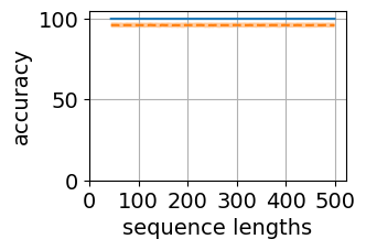
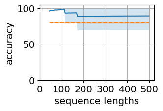
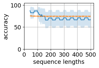
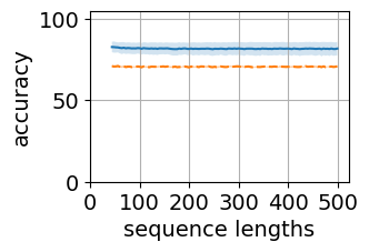
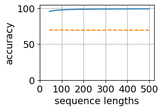
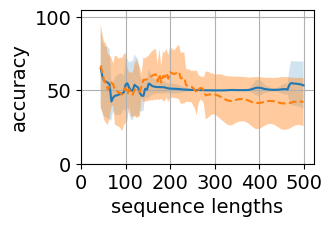
A.1 Generalization Results
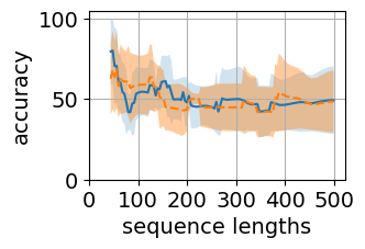
Figure 5 shows the generalization plots for LSTM and O2RNN for both training strategies i.e. all layers trained and classifier-only trained. These networks were trained on string lengths and tested on lengths . The plots show the distribution of performance across the test sequence lengths. Both RNNs maintain their accuracy across the test range indicating generalization of the results.
A.2 Results with Transformers
To examine the capacity of transformer encoder architecture and compare them with our results from RNNs, we train one layer transformer encoder architecture. For binary classification of counter languages, we adopt two different embedding strategies as input to the classifier:
-
1.
transformer-avg : The classification layer receives the mean of all output embeddings generated by the transformer encoder as input feature.
-
2.
transformer-cls : The classification layer receives the output embedding of [CLS] token as input feature.
We train single layer transformer encoder network on two counter languages and . We use the embedding dimension of with attention heads. Table 5 and figure 6 shows that one-layer transformer encoder model fails to learn counter languages. Among the two classification strategies, transformer-cls shows high standard deviation in performance than transformer-avg across seeds. transformer-cls model on some seed performed as high as on grammars, however the mean performance across seeds remained near . transformer-cls model does not show any signs of training (table 4) for weight initialization strategies used for comparing RNNs. For most seeds, the network has accuracy.
A.3 Results on Penn Tree Bank dataset
Table 3 compares O2RNN, LSTM and one-layer transformer encoder network on PTB dataset. O2RNN and LSTM are trained with hidden state size of for character level training, and with size for word level training. For transformer-encoder model we use similar embedding dimensions - for character level training and for word level training.
| dataset | model | all layers | classifier-only | |
|---|---|---|---|---|
| ptb-char | lstm | 3.1243 | 7.7886 | |
| o2rnn | 3.2911 | 8.4865 | ||
|
4.4389 | 9.6622 | ||
| ptb-word | lstm | 160.3073 | 403.9483 | |
| o2rnn | 283.5615 | 356.4486 | ||
|
196.8097 | 318.425 |
| all layers | classifier | |||||
|---|---|---|---|---|---|---|
| initialization | negative samples | model | max | mean ± std | max | mean ± std |
| uniform | hard 0 | lstm | 99.89 | 92.96 ± 13.2 | 95.54 | 94.03 ± 1.48 |
| o2rnn | 99.12 | 99.1 ± 0.01 | 87.54 | 87.5 ± 0.02 | ||
| transformer-cls | 50 | 50.00 ± 0.00 | 50 | 49.99 ± 0.02 | ||
| hard 2 | lstm | 86.96 | 79.33 ± 10.15 | 74.74 | 74.41 ± 0.31 | |
| o2rnn | 85.5 | 82.6 ± 2.93 | 70.72 | 70.66 ± 0.03 | ||
| transformer-cls | 50 | 50.00 ± 0.00 | 50 | 50.00 ± 0.00 | ||
| orthogonal | hard 0 | lstm | 99.99 | 98.64 ± 1.76 | 96.88 | 96.13 ± 0.5 |
| o2rnn | 99.12 | 99.10 ± 0.01 | 87.54 | 87.03 ± 1.41 | ||
| transformer-cls | 53.05 | 50.58 ± 1.0 | 50.22 | 49.99 ± 0.13 | ||
| hard 2 | lstm | 86.55 | 67.85 ± 14.15 | 75.24 | 74.83 ± 0.27 | |
| o2rnn | 85.41 | 80.34 ± 3.36 | 70.72 | 70.25 ± 1.23 | ||
| transformer-cls | 51.23 | 50.15 ± 0.48 | 50.08 | 49.72 ± 0.61 | ||
| sparse | hard 0 | lstm | 99.59 | 99.27 ± 0.16 | 96.55 | 95.85 ± 0.39 |
| o2rnn | 99.12 | 99.10 ± 0.01 | 87.54 | 83.75 ± 11.25 | ||
| transformer-cls | 50 | 50.00 ± 0.00 | 50 | 50.00 ± 0.00 | ||
| hard 2 | lstm | 86.26 | 76.96 ± 13.73 | 76.39 | 72.87 ± 7.63 | |
| o2rnn | 85.66 | 80.50 ± 3.48 | 70.72 | 58.26 ± 10.12 | ||
| transformer-cls | 50 | 50.00 ± 0.00 | 50 | 50.00 ± 0.00 | ||


1
| grammar | feature | layers trained | max | mean ± std |
|---|---|---|---|---|
| cls | all layers | 55.45 | 51.70 ± 2.37 | |
| classifier-only | 60.22 | 49.88 ± 7.40 | ||
| avg-pool | all layers | 58.58 | 51.53 ± 2.44 | |
| classifier-only | 59.15 | 51.60 ± 2.92 | ||
| cls | all layers | 64.25 | 51.99 ± 10.59 | |
| classifier-only | 60.47 | 50.22 ± 9.38 | ||
| avg-pool | all layers | 55.79 | 49.35 ± 3.01 | |
| classifier-only | 52.36 | 49.41 ± 1.27 |
A.4 Stable and Unstable Fixed Points
and are monotonic functions with bounded co-domain. For , both functions are non-decreasing. Let be a monotonic, non-decreasing function with bounded co-domain, and , Then,
-
•
If one fixed point exists, then it is a stable fixed point
Let where is the only fixed point. Then, , thus iteratively , with each and equality occuring at . Similary for , we can show that with each iterative application of , moves towards . -
•
If two fixed points exists, then one fixed point is stable and other is unstable.
If there are two fixed points then at one fixed point () is tangent to . For , thus making that fixed point unstable. -
•
If three fixed point exists, then two fixed points are stable and one is unstable.
This is already shown in Theorem 3.2 and 3.3.
Appendix B: Estimation Methodology based on Machine Precision
Given the constraints of the RNN model and the precision limits of float32, we aim to calculate the maximum distinguishable count for each symbol in the sequence.
Assumptions
-
•
The activation function is used in the RNN, bounding the hidden state outputs within .
-
•
The machine epsilon () for float32 is approximately , indicating the smallest representable change for values around 1.
-
•
A conservative approach is adopted, considering a dynamic range of interest for outputs from -0.9 to 0.9 to avoid saturation effects.
Calculation Dynamic Range and Minimum Noticeable Change The effective dynamic range for outputs is set to avoid saturation, calculated as:
Assuming a minimum noticeable change in the hidden state, given by , to ensure distinguishability within the SGD training process, we have:
Number of Distinguishable Steps The total number of distinguishable steps within the dynamic range can be estimated as:
Given the usable capacity for encoding is potentially less than the total dynamic range due to the RNN’s need to represent sequence information beyond mere counts, a conservative factor () is applied:
Conservative Factor and Final Estimation Applying a conservative factor () to account for the practical limitations in encoding and sequence discrimination, we estimate without dividing by 3, contrary to the previous incorrect interpretation. This factor reflects the assumption that not all distinguishable steps are equally usable for encoding sequences due to the complexity of sequential dependencies and the potential for error accumulation.
Thus we can shown that this estimation provides a mathematical framework for understanding the maximum count that can be distinguished by a simple RNN model with fixed weights and a trainable classification layer, under idealized assumptions about floating-point precision and the behavior of the activation function. The actual capacity for sequence discrimination may vary based on the specifics of the network architecture, weight initialization, and training methodology.
Appendix C: Complete Proofs Precision Theorem
We provide detailed proof for theorem 6.1 presented in the main paper
Proof.
The proof proceeds in three steps: (1) analyzing the hidden state dynamics in the presence of random fixed weights, (2) demonstrating that distinct classes (e.g., ) can still be linearly separable based on the hidden states, and (3) showing that the classification layer can be trained to distinguish these hidden state patterns.
1. Hidden State Dynamics with Fixed Random Weights:
Consider an RNN with hidden state updated as:
where and are randomly initialized and fixed. The hidden state dynamics in this case are governed by the random projections imposed by and .
Although the weights are random, the hidden state still carries information about the input sequence. Specifically, different sequences (e.g., , , and ) induce distinct trajectories in the hidden state space. These trajectories are not arbitrary but depend on the input symbols, even under random weights.
2. Distinguishability of Hidden States for Different Sequence Classes:
Despite the randomness of the weights, the hidden state distributions for different sequences remain distinguishable. For example: - The hidden states after processing tend to cluster in a specific region of the state space, forming a characteristic distribution. - Similarly, the hidden states after processing and will occupy different regions.
These clusters may not correspond to single fixed points as in the trained RNN case, but they still form distinct, linearly separable patterns in the high-dimensional space.
3. Training the Classification Layer:
The classification layer is a fully connected layer that maps the final hidden state to the output class (e.g., ”class 1” for ). The classification layer is trained using a supervised learning approach, typically minimizing a cross-entropy loss.
Because the hidden states exhibit distinct distributions for different sequences, the classification layer can learn to separate these distributions. In high-dimensional spaces, even random projections (as induced by the random recurrent weights) create enough separation for the classification layer to distinguish between different classes.
The main key insight observed based on above analysis is that even with random fixed weights, the hidden state dynamics create distinguishable patterns for different input sequences. The classification layer, which is the only trained component, leverages these patterns to correctly classify sequences like . This demonstrates that the RNN’s expressivity remains sufficient for the classification task, despite the randomness in the recurrent layer.
∎
Now We provide detailed proof for theorem 6.2 presented in the main paper
Proof.
The proof is divided into three parts: (1) establishing the existence of stable fixed points for each input symbol, (2) analyzing the convergence of state dynamics to these fixed points, and (3) demonstrating how the RNN encodes the sequence using these fixed points.
1. Existence of Stable Fixed Points for Each Input Symbol:
Let the hidden state at time be updated according to:
where represents the input symbol. For a fixed input symbol , we analyze the fixed points of the hidden state dynamics.
The fixed points satisfy:
Assume that the system has distinct stable fixed points for inputs , , and , respectively. These fixed points are stable under small perturbations, meaning that for each symbol, the hidden state dynamics tend to converge to the corresponding fixed point.
2. Convergence of State Dynamics to Fixed Points:
For a sufficiently long subsequence of identical symbols, such as , the hidden state will converge to as increases. This convergence is governed by the stability of the fixed point . The same holds true for subsequences and , where the hidden state will converge to and , respectively.
Mathematically, this convergence is characterized by the eigenvalues of the Jacobian matrix at the fixed point :
If the eigenvalues satisfy for all , the fixed point is stable, ensuring that the hidden state dynamics converge to over time.
3. Encoding the Sequence via Fixed Points:
Given a bounded sequence length , the RNN can encode the sequence by leveraging the stable fixed points , , and as follows:
-
1.
After processing the subsequence , the hidden state converges to .
-
2.
Upon receiving the input symbol , the hidden state begins to transition from to . As the network processes , the hidden state stabilizes at .
-
3.
Similarly, the hidden state transitions to after processing , representing the final part of the sequence.
4. Expressivity of RNNs and DFA Equivalence:
The expressivity of RNNs and even o2RNN is equivalent to that of deterministic finite automata (DFA) [2, 5]. In this context, the RNN’s behavior mirrors that of a DFA, with distinct stable fixed points representing states for each input symbol. The transitions between these states are governed by the input sequence and the corresponding hidden state dynamics, which collapse to stable fixed points. This allows the RNN to encode complex grammars like purely through its internal state dynamics.
Thus it can be seen that RNN can encode the sequence by relying on the convergence of state dynamics to stable fixed points. The bounded sequence length ensures that the hidden states have sufficient time to converge to these fixed points, enabling the network to express such grammars within its capacity. The expressivity of the RNN, akin to a DFA, underlines that the encoding is achieved purely through state dynamics, which is especially true for 02RNN.
∎