Precursors of non-Markovianity
Abstract
Using the paradigm of information backflow to characterize a non-Markovian evolution, we introduce so-called precursors of non-Markovianity, i.e. necessary properties that the system and environment state must exhibit at earlier times in order for an ensuing dynamics to be non-Markovian. In particular, we consider a quantitative framework to assess the role that established system-environment correlations together with changes in environmental states play in an emerging non-Markovian dynamics. By defining the relevant contributions in terms of the Bures distance, which is conveniently expressed by means of the quantum state fidelity, these quantities are well defined and easily applicable to a wide range of physical settings. We exemplify this by studying our precursors of non-Markovianity in discrete and continuous variable non-Markovian collision models.
I Introduction
Open quantum systems provide the framework for describing how a system of interest interacts with its surroundings. The ubiquity of this paradigm has led to a wide variety of techniques to model, characterize, and exploit the manner in which an environment affects a system’s evolution Alicki and Lendi (1987); Weiss (1993); Breuer and Petruccione (2002); Rivas and Huelga (2012). In the context of open quantum systems, typically the system of interest is much smaller than its environment and in this case, if the coupling is weak, the dynamics of the system can be well captured by a memoryless or Markovian evolution.
The failure of such an approximation in the presence of strong coupling, structured reservoirs, or non-negligible system effects on the environment, naturally leads us to explore dynamics with some form of memory. Dynamics of this sort are typically referred to by the catch-all term non-Markovianity and have been the subject of intense activity, evidenced by the development of a range of techniques to simulate and characterize a wide range of non-Markovian dynamics, see e.g. the recent reviews Breuer (2012); Breuer et al. (2016); Rivas et al. (2014); de Vega and Alonso (2017); Li et al. (2018). Indeed beyond being a topic of interest in itself, recent work has shown that non-Markovianity of the dynamics can provide an enhancement in a diverse array of settings and tasks, including quantum-metrology, quantum memories, information processing, and thermodynamic cycles Huelga et al. (2012); Chin et al. (2012); Cimmarusti et al. (2015); Pezzutto et al. (2019); Çakmak et al. (2019); Sakuldee et al. (2018); Dong et al. (2018).
Despite the clear relevance of the field and its success in showing potential applications, understanding the fundamental mechanisms and features that give rise to quantum non-Markovianity remains a difficult task. Indeed the very foundations of the theory are still the object of intense investigations Pollock et al. (2018); Taranto et al. (2019), the reason for which is due to the fact that different approaches to defining non-Markovianity have been devised, whose relationship is currently under study Chruscinski et al. (2011); Wißmann et al. (2015); Breuer et al. (2018); Chruscinski et al. (2018).
In this work we attempt to underpin some fingerprints of a non-Markovian evolution by considering precursors of non-Markovianity, i.e. features of the system and environment state at some time, , that serve as necessary (but not sufficient) indicators that the dynamics can show a non-Markovian behavior at a later time . These quantities can be introduced in the framework of non-Markovianity described as a backflow of information from the environment to the system Breuer et al. (2009, 2016). In this picture, bounds can be introduced that explicitly relate the behavior of a particular indicator of non-Markovianity with the features of the joint system-environment state Laine et al. (2010); Amato et al. (2018). Precursors of non-Markovianity provide necessary conditions for tracing revivals in a suitable distinguishability quantifier back to a combination of established system-environment correlations and changes in the environmental state. A significant limitation of the approach is that it calls for evaluation of features of both the system and the total environment, which is generally too demanding a task, and as such investigations along these lines have rarely been considered Mazzola et al. (2012); Rodríguez-Rosario et al. (2012); Smirne et al. (2013). However, it has been shown that when the environment can be described as a collection of individual subsystems, often only a small subset of the total environmental degrees of freedom plays a significant role in driving the evolution Iles-Smith et al. (2014); Campbell et al. (2018). By relying on the Bures distance and considering collision models of open quantum system dynamics Rau (1963); Brun (2002); Scarani et al. (2002); Ziman and Bužek (2005), where the environment is modelled by an ensemble of individual ancillae with which the system sequentially interacts, we are able to introduce and study a hierarchy of precursors of non-Markovianity for systems in both discrete and continuous variable settings. Our work paves the way for considering the relevance of such precursors in a variety of settings which allow for the systematic introduction of environmental degrees of freedom, e.g. within the framework of reaction coordinate models or chain mappings Hughes et al. (2009); Chin et al. (2010); Martinazzo et al. (2011); Woods et al. (2014); Strasberg et al. (2016); Tamascelli et al. (2018a, b).
The remainder of the paper is organized as follows. In Sec. II we define the precursors of non-Markovianity, and in particular the bound, Eq. (2), that is central to our analysis. In Sec. III we apply our framework to both discrete and continuous variable collision models, and qualitatively compare and contrast the emergence of non-Markovianity in the disparate dimensional systems. Finally, in Sec. IV we draw our conclusions.
II Precursors of non-Markovianity
In a seminal work, the non-Markovianity of a reduced quantum dynamics has been introduced as an indicator of information backflow from the environment to the system Breuer et al. (2009). In order to detect and estimate this backflow a distance on the state space, namely the so-called trace distance, has been considered. Apart from a normalization factor, this distance, given for any pair of states and by
corresponds to the natural topology on the state space and has two basic features, which makes it suitable as an estimator of information backflow: (i) it is directly related to a notion of distinguishability among states; (ii) it is a contraction under the action of positive, and in particular completely positive, trace preserving maps. Consequently, it has been possible to consider the evolution in time of the trace distance between two evolved distinct initial states and as an indicator of non-Markovianity, associated to revivals in time of the corresponding trace distance
for some and a pair and , as detailed for example in Ref. Breuer et al. (2016). Revivals in the trace distance correspond to revivals in distinguishability, i.e. the capability to ascertain the actual initial state by performing measurements on the system only. The information backflow associated to these revivals has been traced back to the establishment of correlations between system and environment as well as to changes in the state of the environment.
This notion of information backflow can be formalized as follows. Let us identify the total amount of information at time as the distinguishability of the states of both system and environment
This quantity is a constant and can be naturally written as the sum of two contributions referring to the information that can be obtained by performing local measurements only, namely , and to the residual information which can only be accessed measuring also the environment . While their sum is a constant, i.e.
nevertheless revivals in the internal information can take place, such that for , and they are interpreted as information backflow. This interpretation is substantiated by the following inequality
| (1) |
valid for arbitrary , thus extending previous seminal work on the study of initial correlations Laine et al. (2010); Amato et al. (2018). It appears that to have a local revival of the trace distance at a time greater than , that is a positive contribution on the l.h.s., at least one of the contributions on the r.h.s., referring to time , has to be positive. In this respect such quantities act as precursors of non-Markovianity, in that their positivity at time is a necessary, but not sufficient, condition in order to have a larger trace distance at a later time . Let us further remark that in the case in which the environment is not affected by the system and no correlations are established, corresponding to a perfectly Markovian dynamics, the r.h.s. of the bound is strictly zero, thus forbidding any revival of distinguishability. Evaluation of Eq. (1) is however quite demanding since it calls for the calculation of the trace distance between both system and environment states, where the latter is in general high-dimensional. Indeed, even the evaluation of the trace distance for the system is a difficult task if one considers higher, possibly infinite, dimensional systems. To overcome these difficulties we will consider a different quantifier of the distinguishability among states and build on the structure of the environment in order to obtain alternative bounds, which still provide necessary conditions for the revivals in distinguishability without calling for measurements on both the system and the whole environment.
In order to consider arbitrary dimensional systems it is natural to introduce as a distance on the state space the so-called Bures distance Fuchs and van de Graaf (1999); Vasile et al. (2011)
where denotes fidelity which is readily computable for both finite dimensional and Gaussian continuous variable systems Olivares (2012); Banchi et al. (2015). The Bures distance is indeed a metric on the state space, thus satisfying in particular the triangular inequality, and since it is defined in terms of the fidelity, it is a contraction under the action of completely positive trace preserving maps. These properties together with subadditivity with respect to the tensor product allow to reproduce the inequality Eq. (1) in the form
| (2) |
while retaining its physical interpretation. In this formulation we are, however, still bound to the evaluation of the Bures distance involving all system and environment degrees of freedom, which remains a very difficult task.
We now observe that for the case in which the environment exhibits a natural structuring in terms of constituent subunits (ancillae), as is the case in collision models Scarani et al. (2002); Ziman and Bužek (2005), we can construct a hierarchy of environmental marginals by taking the partial trace with respect to a growing number of environmental ancillae. Exploiting the fact that the partial trace is indeed a completely positive trace preserving transformation, supposing the environment to be composed of ancillae we have the following chain of bounds for the quantifier of correlations
| (3) |
For we recover the original upper bound , while for we have the trivial bound . Similarly, for the difference in environmental states we have
| (4) |
Thus, it immediately appears that the different terms at the r.h.s. of Eq. (2) can be lower bounded by a whole hierarchy of positive quantities obtained by replacing the environmental states with suitable marginals obtained by tracing out different ancillae. In such a way one can obtain precursors of non-Markovianity which can be more easily evaluated. It is important to stress however that all of these quantities provide lower bounds for the r.h.s., corresponding to quantities which are increasingly easier to evaluate. In this respect, while strict positivity of either of these quantities provides a necessary condition for revivals of Bures distance between distinct pair of initial system states, lower bounding the r.h.s. might lead to a violation of the bound Eq. (2), in the sense that the lower bound for the r.h.s. of Eq. (2) is no longer an upper bound to the l.h.s. On the other hand, as we will show in the collision framework in Sec. III, it turns out that even the simplest approximation can already lead to a very good estimate of Bures distance revivals. Indeed as shown in Sec. III.3, in the collision model framework it appears that already the “minimal approximation” for the environment, treated as being a single ancilla, actually provides quite reasonable bounds, indicating that the contributions arising from the system interacting with this particular ancilla are the most relevant ones for characterizing the dynamics. This is complementary to Ref. Campbell et al. (2018) from which we know that the incoming single ancilla is the only really relevant player in dictating the non-Markovianity of the evolution in the corresponding collision model.
We remark that our choice of the Bures distance over other metrics goes beyond its comparative computational simplicity and applicability to infinite dimensional settings already mentioned. The crucial property that any candidate distinguishability measure must have is to be a contraction under the action of completely positive trace preserving maps. While this condition is met for the Bures and trace distances, other norms, such as the Hilbert-Schmidt norm, fail to satisfy it Wang and Schirmer (2009) and thus make them unsuitable choices. Moreover, in order to explicitly relate the bounds to physically meaningful notions, i.e. the established system-environment correlations or environmental changes, one requires a norm so as to exploit the triangular inequality. This requirement therefore rules out quantifiers such as the relative entropy. For these reasons the Bures distance emerges as the most natural metric for the task at hand.
III Application to a Collision Model
Let us begin by outlining the basic collision model framework Scarani et al. (2002); Ziman and Bužek (2005); McCloskey and Paternostro (2014); Kretschmer et al. (2016); Çakmak et al. (2017); Campbell et al. (2018); Jin and Yu (2018); Strasberg et al. (2017); Ciccarello (2018) which provides a versatile tool for exploring the emergence of non-Markovianity and, due to their construction, serves as the ideal testbed for studying the precursors of non-Markovianity captured in Eq. (2) by exploiting Eqs. (3) and (4). Following Refs. McCloskey and Paternostro (2014); Campbell et al. (2018), the environment is composed of an array of individual ancillae, , initially factorized and all with the same initial state. The time evolution is discretized such that at “time-step” the system, , collides with ancilla, , after which we retain all correlations established by this system-ancilla (SA) interaction while subsequently collides with . At this point we can trace out the degrees of freedom associated with , after which we begin time-step where the system collides with and so on. Due to the intra-environment ancilla-ancilla (AA) collisions, i.e. -, may already share some correlations with before they interact McCloskey and Paternostro (2014); Campbell et al. (2018). Furthermore, due to the AA collision the incoming state of the ancilla, , that the system interacts with is not typically its initialized state. Thus, the collision model provides a natural setting to explore non-Markovianity arising due to both the establishment of correlations between system and environment together with changes in the state of the environment, as discussed in Sec. II and captured succinctly by Eq. (2).
As shown in Ref. Campbell et al. (2018), when we restrict to only nearest neighbor AA interactions this corresponds to a memory depth of one and is termed “first-order Markovian” since we need only concern ourselves with keeping track of the system and one additional ancilla to faithfully simulate of the dynamics. Thus, the evolution follows as
| (5) | |||||
where denotes the initial ancilla state. We exactly recover the standard evolution according to the Markovian master equation when there are no AA collisions, under the condition that the unitary is an energy preserving exchange interaction and all constituents have the same free Hamiltonian terms McCloskey and Paternostro (2014); Pezzutto et al. (2016). Despite the framework is independent of the dimensionality of system and ancilla, most studies restrict to the discrete variable qubit states McCloskey and Paternostro (2014); Kretschmer et al. (2016); Campbell et al. (2018); Çakmak et al. (2017), with only a few exceptions Jin and Yu (2018). Therefore in this work, we are interested in examining any effect that dimensionality may have on the properties of the non-Markovian dynamics, and on the precursors of non-Markovianity, by comparing and contrasting when system and ancilla are discrete variable (DV) qubits with when they are continuous variable (CV) Gaussian states.
When considering the DV case the interaction will be given by the energy preserving partial swap operation
| (6) |
with
| (7) |
We will allow for a generic pure, real initial state of the system, written in the ordered basis ,
| (8) |
For the CV setting we will assume that SA collisions are described by a beamsplitter
| (9) |
whereas AA collisions are defined by
We observe that : the beam splitter implementing the AA interaction has reflectivity and transmittivity inverted w.r.t. the beam splitter realizing the SA interaction. This corresponds to the shift of a phase factor from the second environmental mode to the first one and allows to avoid a “jagged” behaviour of the covariance matrix phases (see Jin and Yu (2018)). We will consider thermal squeezed initial states for the system with covariance matrices given by
| (10) |
In what follows we will initialize all environmental ancillae in their ground, respectively vacuum, state for both the DV and CV settings and we will fix the SA (AA) interaction strengths, Eqs. (6) and (9), for both the DV and CV cases to be (). The energy preserving nature of the interaction ensures that the steady-state of system is driven to is exactly the initial state of one of the environmental ancillae, i.e. .
III.1 Discrete Variable case
(a)
(b)
(c)
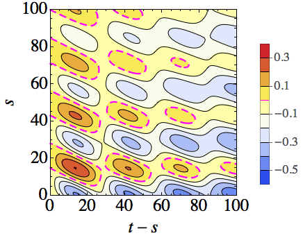
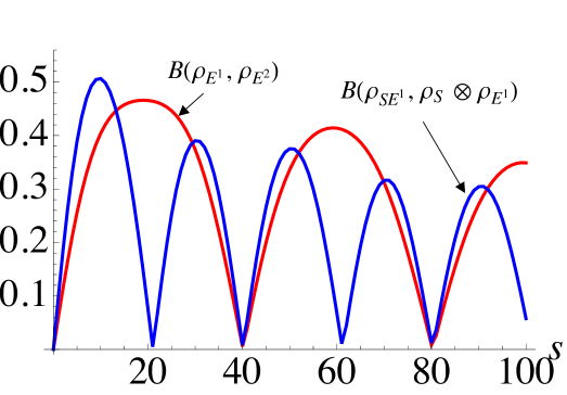
For the DV setting we fix the initial state of all ancillae to be and, in order to evaluate Eq. (2), we consider the two initial system states to be and . Since is already the steady state of the dynamics, no evolution takes place. This simplifies our evaluation of the various components entering into Eq. (2) since the third term on the r.h.s. will be identically zero. Nevertheless we can analyze the non-Markovian dynamics arising in this picture as shown in Fig. 1. Panel (a) shows the l.h.s of Eq. (2), which accounts only for changes in the system states. As noted previously, we can associate positive values of this quantity with a backflow of information to the environment and therefore periods of non-Markovianity. These periods of non-Markovianity are captured within the dashed, magenta contours. Consider first fixing , we see from the ensuing evolution in that the l.h.s of Eq. (2) remains negative for all , corresponding to the absence of initial correlations. In contrast, if we consider larger values of we observe that for revivals can appear. We can clearly see that there is a natural periodicity in these revivals when we witness regions of non-Markovianity in terms of the “reference-time” . Furthermore, we see the magnitude of the revivals diminishes as increases, which is to be expected since the state of the system is always driven towards the steady state .
We can understand these features by examining our precursors of non-Markovianity. Turning our attention to Fig. 1 (b) we consider the r.h.s of Eq. (2) where, by exploiting the hierarchy of bounds in Eqs. (3) and (4), we approximate the environment to be a single ancilla, which for a given step is the state of , i.e. the state of the incoming ancilla after both the SA and AA collisions have taken place. We see that the contributions entering Eq. (2) behave qualitatively the same. In particular, focusing on the extremal behaviours we clearly see that when the contributions are largest for a given , this corresponds precisely to when the strongest non-Markovian revivals are present in the l.h.s of Eq. (2) for some . We further put this behavior into evidence in panel (c) where we combine the data from the preceding panels.
From these results we can conclude that in the DV case the contributing factors leading to a non-Markovian evolution appear equally important. We can clearly see from panel (c) that large revivals in the l.h.s of Eq. (2) are associated with both significant amounts of established correlations between system and incoming ancilla and with significant changes to the incoming ancilla state from its initial configuration.
III.2 Gaussian continuous variable case
While considerably less well studied, the case of CV collision models provides an interesting platform for the realization and study of non-Markovianity, particularly in light of the remarkable advances in the manipulation of CV systems for simulating open quantum system dynamics Chiuri et al. (2012); Ciampini et al. (2018); Cuevas et al. (2019). Inline with the DV analysis, we initialize all ancillary modes in the vacuum state. In order to evaluate Eq. (2), we again require two initial system states. Similarly to the previous analysis we fix to be the vacuum state such that no dynamics will occur in this case, thus simplifying the evaluation of Eq. (2) since the third term will again be identically zero. At variance with the DV case, we cannot readily initialize our system in a state orthogonal to . However, we can consider a strongly squeezed vacuum state, setting and in Eq. (10), which is sufficient for our purposes.
(a)
(b)
(c)
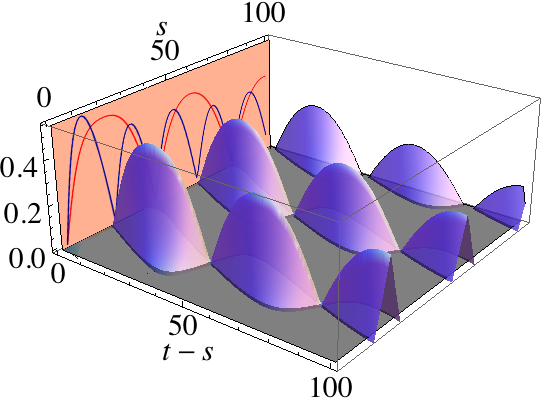
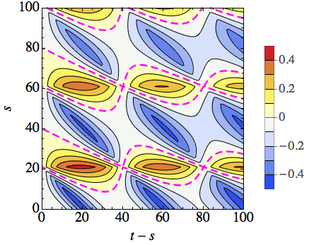
In Fig. 2 (a) we evaluate the l.h.s of Eq. (2). Immediately we can note that there are a number of qualitative similarities with the DV setting. In particular, the clear periodicity in the emergence of regions of non-Markovianity and the decreasing amplitude of the revivals for increasing . However, in contrast with the DV case, we now see that there are special values of which correspond to continual periods of non-Markovianity. For the considered parameters, fixing to 20, 60, or 100 collisions we see that the ensuing dynamics is always non-Markovian, while for equal to 0, 40, or 80 the dynamics is always Markovian. Such a behavior is notably different to the DV case where periods of non-Markovianity are always followed by at least a short period of Markovianity, regardless of the value of .
This behavior is captured by Fig. 2 (b) where we show the contributions from the r.h.s of Eq. (2). In contrast with the DV case, we now see that the term capturing correlations and the term encompassing environmental changes contribute in a strikingly different manner. In particular, the correlations established between the system and the environment have double the period compared with the changes in the incoming environmental state. This has consequences when we examine the apparent causes of the most non-Markovian regions of Fig. 2 (a). For the considered parameters, when we find that for , the l.h.s of Eq. (2) achieves its largest revivals. This corresponds to when the first term on the r.h.s. of Eq. (2), related to the change in the incoming environmental state, is at its maximum, while the second term related to the correlations shared between the system and environment is zero.
A qualitatively similar behavior to the DV case can be seen considering a “reference-time” for which the contributions entering into the r.h.s of Eq. (2) are large and comparable in magnitude. We again further put into evidence the relation between the precursors of non-Markovianity and the ensuing non-Markovian dynamics in in panel (c).
III.3 Validity of the Environmental-Size Approximation
(a)
(b)
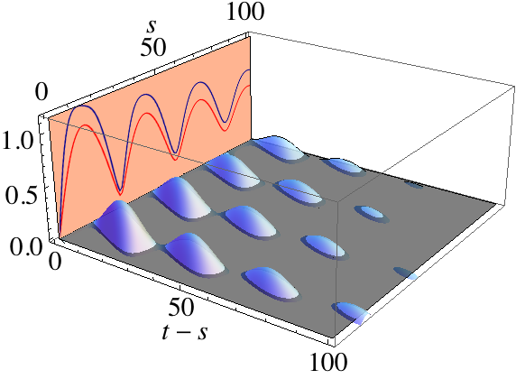
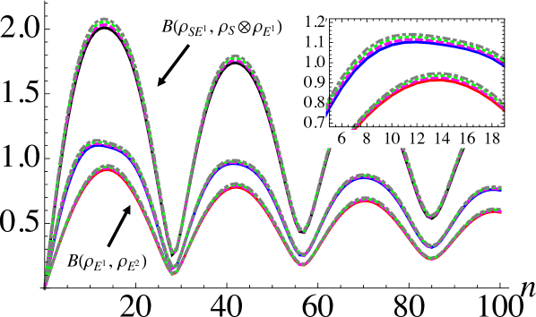
In the preceding analyses, to evaluate Eq. (2) we made the rather strong assumption that only a single environment ancilla was needed. In particular, we assumed that the incoming ancilla encapsulated all the relevant information to determine the bounds. Here we consider a more careful analysis of the validity of this approximation. To this end we simply examine how the various quantities on the r.h.s of Eq. (2) are affected when more environmental degrees of freedom are kept during the simulation. It should be noted that since all quantities are positive, the minimal values observed for only a single ancilla approximation for the environment have already proven to be remarkably good bounds. Indeed, examining Figs. 1 and 2 we see that even with such an extreme approximation we achieve meaningful and insightful bounds. Furthermore as shown in Ref. Campbell et al. (2018), since we know that the dynamics are unaffected by storing more ancillae (and their associated correlations) beyond the memory depth, one might expect that the approximated bounds studied previously are robust. In Fig. 3 we show that this is indeed the case. The inclusion of more environmental ancillae has only a small effect on the values of the various contributions entering into the r.h.s of Eq. (2). Here we see that the consideration of additional environmental degrees of freedom that are no longer playing an active role in dictating the dynamics of the system provide only a minor contribution to the precursors of non-Markovianity. The seemingly small contribution of these additional correlations can be understood due to the fact that, despite not playing a role in the dynamics, all previously interacted with ancillae share some correlation with the system throughout the entire dynamics Campbell et al. (2018). While these correlations appear to be small, they still provide a non-zero contribution to the bounds. These contributions persist until the the system has fully equilibrated with the environment, which corresponds to when the system reaches a factorized state with the environment Cusumano et al. (2018).
III.4 Non-Markovianity in discrete versus continuous variable models
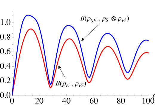
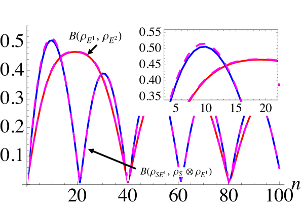
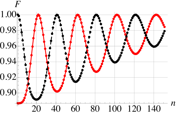
We have established that while DV and CV settings share several qualitative features, there are notable differences arising. In particular, with regards to the precursors of non-Markovianity we have seen that the various contributions behave quite differently in the two disparate dimensional settings. We can gain a better understanding of the differences between the two settings by considering how close the system gets to the steady state during the dynamics. In Fig. 4 the lighter, colored curves show the fidelity between the system when it is initialized in with the steady state , while the black curves show the fidelity of the incoming ancilla with . In panel (a) for the DV case we see that the system slowly approaches the steady state, while the incoming ancilla periodically approaches close to its initial state. In contrast, for the CV case in panel (b) we see that the system transients the steady state repeatedly during the dynamics, and similarly the incoming ancilla also periodically returns precisely to its initial state, despite the AA collisions having taken place.
(a)
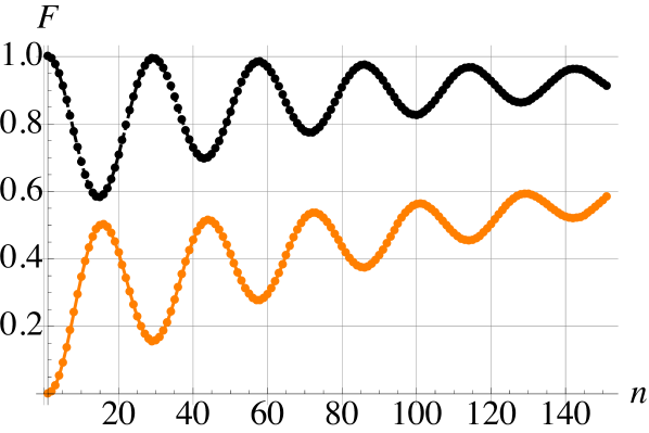
(b)
The different behavior of the precursors of non-Markovianity between our considered settings also leads to a final interesting difference. As shown in Ref. McCloskey and Paternostro (2014), a weaker form of non-Markovianity can still be witnessed in the DV collision model if, after the SA collision, the correlations shared between system and ancilla are erased before the AA interaction takes place. In order to see a non-Markovian dynamics however, the initial state of the system must have some coherence, e.g. the system should be initialized in and/or . Interestingly, if we consider the same correlation erasure scheme in the CV case, we find that the dynamics is always Markovian, even for strongly squeezed initial system states.
We remark that, while we presented results referring to zero-temperature environment here, the behaviours described above remain qualitatively the same for different environmental temperatures and different initial states of the system and of the incoming ancillae.
IV Conclusions
The description of non-Markovianity of quantum dynamics being due to an information backflow between system and environment leads us to identify the establishment of system-environment correlations and changes in the state of the environment as sources of non-Markovian behavior. In the trace distance approach to non-Markovianity, a bound can be introduced to relate revivals of distinguishability to such changes. We have reformulated this bound in terms of the Bures distance, which is based on the quantum state fidelity. This allows to assess a greater range of physical systems since the fidelity is comparatively easier to compute than the trace distance, in particular when one wishes to consider infinite dimensional systems. Revivals in the l.h.s of the bound, indicating periods of non-Markovianity, can be understood in terms of different contributions due to system-environment correlations and changes in the environmental state at an earlier time, thus establishing the r.h.s of the bound as capturing precursors of non-Markovianity. We have shown that the evaluation of these precursors of non-Markovianity can be simplified when the environment can be decomposed into smaller constituent parts, thus leading to a strategy of general applicability. This is possible by considering a hierarchy of lower bounds to the bound in Bures distance revivals set by the overall amount of established correlations and changes in environmental state. Such lower bounds can be considered whenever the environment exhibits a natural partition within its Hilbert space. We applied this framework to a collision model, where we explored both discrete variable (DV) and continuous variable (CV) settings. Exploiting the considered bound we established that the causes of non-Markovianity in such a collision model showed some qualitative differences between the two disparate dimensional settings, in particular while in the DV case the various contributions to non-Markovianity behaved largely the same, we found that the precursors of non-Markovianity exhibited quite a different behavior in the CV setting. While our results were based on zero-temperature environments, we stress that the same features persist for finite temperature environments and for other choices of initial system states. Our results provide a useful tool for studying the causes of a non-Markovian evolution based on readily computable quantities. Furthermore, we believe our analysis is one of the first to comparatively assess the effect that dimensionality can have on the ensuing non-Markovian character of a given evolution.
Acknowledgements.
SC gratefully acknowledges the Science Foundation Ireland Starting Investigator Research Grant “SpeedDemon” (No. 18/SIRG/5508) for financial support. MP is supported by funding from the European Research Council (ERC) under the European Union’s Horizon 2020 research and innovation program (ODYSSEY grant agreement No. 758403). BV gratefully acknowledges support from the Joint Project ”Quantum Information Processing in Non- Markovian Quantum Complex Systems” funded by FRIAS/University of Freiburg and IAR/Nagoya University. BV further acknowledges support from the FFABR project of MIUR and from the UniMi Transition Grant H2020.References
- Alicki and Lendi (1987) R. Alicki and K. Lendi, Quantum Dynamical Semigroups and Applications, Lecture Notes in Physics, Vol. 286 (Springer, Berlin, 1987).
- Weiss (1993) U. Weiss, Quantum Dissipative Systems (World Scientific, Singapore, 1993).
- Breuer and Petruccione (2002) H.-P. Breuer and F. Petruccione, The Theory of Open Quantum Systems (Oxford University Press, Oxford, 2002).
- Rivas and Huelga (2012) A. Rivas and S. F. Huelga, Open Quantum Systems: An Introduction (Springer, 2012).
- Breuer (2012) H.-P. Breuer, “Foundations and measures of quantum non-markovianity,” J. Phys. B 45, 154001 (2012).
- Breuer et al. (2016) H.-P. Breuer, E.-M. Laine, J. Piilo, and B. Vacchini, “Colloquium : Non-markovian dynamics in open quantum systems,” Rev. Mod. Phys. 88, 021002 (2016).
- Rivas et al. (2014) A. Rivas, S. F. Huelga, and M. B. Plenio, “Quantum non-markovianity: Characterization, quantification and detection,” Rep. Prog. Phys. 77, 094001 (2014).
- de Vega and Alonso (2017) I. de Vega and D. Alonso, “Dynamics of non-markovian open quantum systems,” Rev. Mod. Phys. 89, 015001 (2017).
- Li et al. (2018) L. Li, M. J. W. Hall, and H. M. Wiseman, “Concepts of quantum non-markovianity: A hierarchy,” Physics Reports 759, 1 – 51 (2018).
- Huelga et al. (2012) S. F. Huelga, Á. Rivas, and M. B. Plenio, “Non-markovianity-assisted steady state entanglement,” Phys. Rev. Lett. 108, 160402 (2012).
- Chin et al. (2012) A. W. Chin, S. F. Huelga, and M. B. Plenio, “Quantum metrology in non-markovian environments,” Phys. Rev. Lett. 109, 233601 (2012).
- Cimmarusti et al. (2015) A. D. Cimmarusti, Z. Yan, B. D. Patterson, L. P. Corcos, L. A. Orozco, and S. Deffner, “Environment-assisted speed-up of the field evolution in cavity quantum electrodynamics,” Phys. Rev. Lett. 114, 233602 (2015).
- Pezzutto et al. (2019) M. Pezzutto, M. Paternostro, and Y. Omar, “An out-of-equilibrium non-Markovian Quantum Heat Engine,” Quantum Sci. Technol. 4, 025002 (2019).
- Çakmak et al. (2019) B. Çakmak, S. Campbell, B. Vacchini, Ö. E. Müstecaplıoğlu, and M. Paternostro, “Robust multipartite entanglement generation via a collision model,” Phys. Rev. A 99, 012319 (2019).
- Sakuldee et al. (2018) F. Sakuldee, S. Milz, F. A. Pollock, and K. Modi, “Non-markovian quantum control as coherent stochastic trajectories,” J. Phys. A: Math. Theor. 51, 414014 (2018).
- Dong et al. (2018) Y. Dong, Y. Zheng, S. Li, C.-C. Li, X.-D. Chen, G.-C. Guo, and F.-W. Sun, “Non-markovianity-assisted high-fidelity deutsch-jozsa algorithm in diamond,” npj Quantum Inf. 4, 3 (2018).
- Pollock et al. (2018) F. A. Pollock, C. Rodriguez-Rosario, T. Frauenheim, M. Paternostro, and K. Modi, “Operational markov condition for quantum processes,” Phys. Rev. Lett. 120, 040405 (2018).
- Taranto et al. (2019) P. Taranto, S. Milz, F. A. Pollock, and K. Modi, “Structure of quantum stochastic processes with finite markov order,” Phys. Rev. A 99, 042108 (2019).
- Chruscinski et al. (2011) D. Chruscinski, A. Kossakowski, and A. Rivas, “On measures of non-markovianity: divisibility vs. backflow of information,” Phys. Rev. A 83, 052128 (2011).
- Wißmann et al. (2015) S. Wißmann, H.-P. Breuer, and B. Vacchini, “Generalized trace-distance measure connecting quantum and classical non-markovianity,” Phys. Rev. A 92, 042108 (2015).
- Breuer et al. (2018) H.-P. Breuer, G. Amato, and B. Vacchini, “Mixing-induced quantum non-markovianity and information flow,” New J. Phys. 20, 043007 (2018).
- Chruscinski et al. (2018) D. Chruscinski, Á. Rivas, and E. Størmer, “Divisibility and information flow notions of quantum markovianity for noninvertible dynamical maps,” Phys. Rev. Lett. 121, 080407 (2018).
- Breuer et al. (2009) H.-P. Breuer, E.-M. Laine, and J. Piilo, “Measure for the degree of non-markovian behavior of quantum processes in open systems,” Phys. Rev. Lett. 103, 210401 (2009).
- Laine et al. (2010) E.-M. Laine, J. Piilo, and H.-P. Breuer, “Witness for initial system-environment correlations in open system dynamics,” EPL 92, 60010 (2010).
- Amato et al. (2018) G. Amato, H.-P. Breuer, and B. Vacchini, “Generalized trace distance approach to quantum non-markovianity and detection of initial correlations,” Phys. Rev. A 98, 012120 (2018).
- Mazzola et al. (2012) L. Mazzola, C. A. Rodríguez-Rosario, K. Modi, and M. Paternostro, “Dynamical role of system-environment correlations in non-markovian dynamics,” Phys. Rev. A 86, 010102 (2012).
- Rodríguez-Rosario et al. (2012) C. A Rodríguez-Rosario, K. Modi, L. Mazzola, and A. Aspuru-Guzik, “Unification of witnessing initial system-environment correlations and witnessing non-markovianity,” EPL 99, 20010 (2012).
- Smirne et al. (2013) A. Smirne, L. Mazzola, M. Paternostro, and B. Vacchini, “Interaction-induced correlations and non-markovianity of quantum dynamics,” Phys. Rev. A 87, 052129 (2013).
- Iles-Smith et al. (2014) J. Iles-Smith, N. Lambert, and A. Nazir, “Environmental dynamics, correlations, and the emergence of noncanonical equilibrium states in open quantum systems,” Phys. Rev. A 90, 032114 (2014).
- Campbell et al. (2018) S. Campbell, F. Ciccarello, G. M. Palma, and B. Vacchini, “System-environment correlations and markovian embedding of quantum non-markovian dynamics,” Phys. Rev. A 98, 012142 (2018).
- Rau (1963) J. Rau, “Relaxation phenomena in spin and harmonic oscillator systems,” Phys. Rev. 129, 1880–1888 (1963).
- Brun (2002) T. A. Brun, “A simple model of quantum trajectories,” Am. J. Phys. 70, 719–737 (2002).
- Scarani et al. (2002) V. Scarani, M. Ziman, P. Štelmachovič, N. Gisin, and V. Bužek, “Thermalizing quantum machines: Dissipation and entanglement,” Phys. Rev. Lett. 88, 097905 (2002).
- Ziman and Bužek (2005) M. Ziman and V. Bužek, “All (qubit) decoherences: Complete characterization and physical implementation,” Phys. Rev. A 72, 022110 (2005).
- Hughes et al. (2009) K. H. Hughes, C. D. Christ, and I. Burghardt, “Effective-mode representation of non-markovian dynamics: A hierarchical approximation of the spectral density. i. application to single surface dynamics,” J. Chem. Phys. 131, 024109 (2009).
- Chin et al. (2010) A. W. Chin, A. Rivas, S. F. Huelga, and M. B. Plenio, “Exact mapping between system-reservoir quantum models and semi-infinite discrete chains using orthogonal polynomials,” J. Math. Phys. 51, 092109 (2010).
- Martinazzo et al. (2011) R. Martinazzo, B. Vacchini, K. H. Hughes, and I. Burghardt, “Universal markovian reduction of brownian particle dynamics,” J. Chem. Phys. 134, 011101 (2011).
- Woods et al. (2014) M. P. Woods, R. Groux, A. W. Chin, S. F. Huelga, and M. B. Plenio, “Mappings of open quantum systems onto chain representations and markovian embeddings,” J. Math. Phys. 55, 032101 (2014).
- Strasberg et al. (2016) P. Strasberg, G. Schaller, N. Lambert, and T. Brandes, “Nonequilibrium thermodynamics in the strong coupling and non-markovian regime based on a reaction coordinate mapping,” New J. Phys. 18, 073007 (2016).
- Tamascelli et al. (2018a) D. Tamascelli, A. Smirne, S. F. Huelga, and M. B. Plenio, “Nonperturbative treatment of non-markovian dynamics of open quantum systems,” Phys. Rev. Lett. 120, 030402 (2018a).
- Tamascelli et al. (2018b) D. Tamascelli, A. Smirne, S. F. Huelga, and M. B. Plenio, “Efficient simulation of finite-temperature open quantum systems,” arXiv:1811.12418 (2018b).
- Fuchs and van de Graaf (1999) C. A. Fuchs and J. van de Graaf, “Cryptographic distinguishability measures for quantum-mechanical states,” IEEE Trans. Inf. Th. 45, 1216–1227 (1999).
- Vasile et al. (2011) R. Vasile, S. Maniscalco, M. G. A. Paris, H.-P. Breuer, and J. Piilo, “Quantifying non-markovianity of continuous-variable gaussian dynamical maps,” Phys. Rev. A 84, 052118 (2011).
- Olivares (2012) S. Olivares, “Quantum optics in the phase space,” Eur. Phys. J. Special Topics 203, 3?24 (2012).
- Banchi et al. (2015) L. Banchi, S. L. Braunstein, and S. Pirandola, “Quantum fidelity for arbitrary gaussian states,” Phys. Rev. Lett. 115, 260501 (2015).
- Wang and Schirmer (2009) X. Wang and S. G. Schirmer, “Contractivity of the hilbert-schmidt distance under open-system dynamics,” Phys. Rev. A 79, 052326 (2009).
- McCloskey and Paternostro (2014) R. McCloskey and M. Paternostro, “Non-markovianity and system-environment correlations in a microscopic collision model,” Phys. Rev. A 89, 052120 (2014).
- Kretschmer et al. (2016) S. Kretschmer, K. Luoma, and W. T. Strunz, “Collision model for non-markovian quantum dynamics,” Phys. Rev. A 94, 012106 (2016).
- Çakmak et al. (2017) B. Çakmak, M. Pezzutto, M. Paternostro, and Ö. E. Müstecaplıoğlu, “Non-markovianity, coherence, and system-environment correlations in a long-range collision model,” Phys. Rev. A 96, 022109 (2017).
- Jin and Yu (2018) J. Jin and C.-S. Yu, “Non-markovianity in a collision model with environmental block,” New J. Phys. 20, 053026 (2018).
- Strasberg et al. (2017) P. Strasberg, G. Schaller, T. Brandes, and M. Esposito, “Quantum and information thermodynamics: A unifying framework based on repeated interactions,” Phys. Rev. X 7, 021003 (2017).
- Ciccarello (2018) F. Ciccarello, “Collision models in quantum optics,” Quantum Meas. Quantum Metrol. 4, 53 (2018).
- Pezzutto et al. (2016) M. Pezzutto, M. Paternostro, and Y. Omar, “Implications of non-Markovian quantum dynamics for the Landauer bound,” New J. Phys. 18, 123018 (2016).
- Chiuri et al. (2012) A. Chiuri, C. Greganti, L. Mazzola, M. Paternostro, and P. Mataloni, “Linear optics simulation of quantum non-markovian dynamics,” Sci. Rep. 2, 968 (2012).
- Ciampini et al. (2018) M. A. Ciampini, G. Pinna, P. Mataloni, and M. Paternostro, “Experimental signature of quantum darwinism in photonic cluster states,” Phys. Rev. A 98, 020101 (2018).
- Cuevas et al. (2019) A. Cuevas, A. Geraldi, C. Liorni, L. D. Bonavena, A. De Pasquale, F. Sciarrino, V. Giovannetti, and P. Mataloni, “All-optical implementation of collision-based evolutions of open quantum systems,” Sci. Rep. 9, 3205 (2019).
- Cusumano et al. (2018) S. Cusumano, V. Cavina, M. Keck, A. De Pasquale, and V. Giovannetti, “Entropy production and asymptotic factorization via thermalization: A collisional model approach,” Phys. Rev. A 98, 032119 (2018).