Predicting speech intelligibility in older adults for speech enhancement using the
Gammachirp Envelope Similarity Index, GESI 11footnotemark: 1
Abstract
We propose an objective intelligibility measure (OIM), called the Gammachirp Envelope Similarity Index (GESI), that can predict speech intelligibility (SI) in older adults. GESI is a bottom-up model based on psychoacoustic knowledge from the peripheral to the central auditory system. It computes the single SI metric using the gammachirp filterbank (GCFB), the modulation filterbank, and the extended cosine similarity measure. It takes into account not only the hearing level represented in the audiogram, but also the temporal processing characteristics captured by the temporal modulation transfer function (TMTF). To evaluate performance, SI experiments were conducted with older adults of various hearing levels using speech-in-noise with ideal speech enhancement on familiarity-controlled Japanese words. The prediction performance was compared with HASPIw2, which was developed for keyword SI prediction. The results showed that GESI predicted the subjective SI scores more accurately than HASPIw2. GESI was also found to be at least as effective as, if not more effective than, HASPIv2 in predicting English sentence-level SI. The effect of introducing TMTF into the GESI algorithm was insignificant, suggesting that TMTF measurements and models are not yet mature. Therefore, it may be necessary to perform TMTF measurements with bandpass noise and to improve the incorporation of temporal characteristics into the model.
keywords:
Speech intelligibility; Hearing loss; Objective intelligibility measure; Auditory model; Speech enhancement; Ideal ratio masker;1 Introduction
The number of older adults is increasing in many countries. As a result, the number of people with age-related hearing loss (HL) is expected to increase. HL impairs speech communication, which is the basis of human interaction, and leads to a decline in quality of life (QOL). The Lancet Committee [Livingston et al., 2024] has also reported that HL is one of the major modifiable risk factors for dementia, highlighting the importance of early intervention. Hearing aids are one of the most important solutions for age-related HL today. However, not everyone with HL uses them. For example, the usage rate is around 40% to 50% in European countries, whereas in Japan it is only 15% [Anovum, 2022]. Furthermore, satisfaction levels among wearers are lower in Japan, at around 50%, compared with over 70% in European countries. This may be due to differences in policy, medical approach and issues such as cost. Ultimately, however, it may also be because hearing aids do not yet provide sufficient performance to compensate for HL.
To solve this problem, it is now critical to develop the next generation of assistive listening devices that can compensate for the difficulties experienced by people with HL. Speech enhancement (SE) and noise reduction algorithms [Loizou, 2013] need to become more robust and effective based on individual hearing characteristics. For algorithm evaluation, subjective listening tests to measure speech intelligibility (SI) are essential, but time-consuming and costly. Therefore, it is important to develop an effective objective intelligibility measure (OIM) that can predict SI for listeners with individually different HL.
Many OIMs have been proposed to evaluate SI when using SE and noise reduction algorithms [Falk et al., 2015, Van Kuyk et al., 2018]. STOI [Taal et al., 2011] and ESTOI [Jensen & Taal, 2016] have been used for this purpose in many studies. GEDI has also been proposed for more conservative evaluation [Yamamoto et al., 2020]. They are intrusive methods that use both the unprocessed or clean reference signal and the test signal to compute the metric. They provide a single metric value that can be converted to the SI scores of speech sounds with a monotonic function such as a sigmoid or cumulative Gaussian. Because of this simplicity, many studies compare the proposed and conventional SE algorithms directly using this metric, without converting to an objective SI score, which requires some human SI data. Although these OIMs work well for predicting SI in normal hearing (NH) listeners, they cannot predict SI in people with varying degrees of HL who truly need good hearing assistive devices.
There are some OIMs that can take the HL into account. Kates & Arehart [2014] proposed HASPI to predict the SI of listeners with HL when using hearing aids. One reason may be that the prediction by this version of HASPI, which provides two or more independent metrics, requires some subjective SI scores. The SI score is calculated by the weighted sum of these metrics with a sigmoid function, and the weights could only be estimated by subjective SI scores.
More recently, by extending the algorithm in GEDI, a new OIM called GESI (Gammachirp Envelope Similarity Index) has been proposed to provide a single metric suitable for such SE evaluations [Irino et al., 2022, Yamamoto et al., 2023]. These OIMs can reflect the hearing level and the degradation factors of the active mechanism of the cochlea. They are based on an auditory filterbank, some form of temporal modulation analysis, feature extraction, and correlation or similarity between the reference and test signals. The metric is derived solely from bottom-up features extracted by an auditory model, using a small number of explicitly defined and interpretable parameters.
This approach contrasts with the method of training a neural network (NN) using parallel data of sounds and subjective SI scores, as in HASPI version 2 [Kates & Arehart, 2021], HASPI w2 [Kates, 2023], and more recent deep neural network (DNN) models (e.g., Huckvale & Hilkhuysen 2022, Tu et al. 2022, Kamo et al. 2022). Clarity Prediction Challenge (CPC) [Barker et al., 2022, 2024] promoted such machine learning OIMs for SI prediction of listeners with HL. The DNN models outperform the simple bottom-up OIMs with the effect of learning algorithms with massive amounts of training data. However, it is well known that the range of good performance is usually limited by the prepared training data, computing power, and memory. In addition, the derived system is a black box, and it is difficult to analyze how the objective SI score is calculated for individual HL listeners. Moreover, the OIMs with NNs and DNNs use a large number of uninterpretable parameters, and their values are derived from learning, including higher-order knowledge, such as contextual information within a sentence. Therefore, there may not be a simple monotonic relationship between the improvement due to signal processing and the predicted SI score derived from them. This may be especially true when overfitting the training data or in untrained conditions. In other words, it may be difficult to interpret the effect of signal processing from the SI scores.
In contrast, OIMs that model bottom-up auditory signal processing provide better insight into how specific dysfunctions affect the SI of listeners with HL. With an OIM consisting only of interpretable parameters, the mapping between the degree of performance improvement achieved through signal processing and the predicted SI scores is expected to be simpler and easier to understand than when using NNs and DNNs. Furthermore, the bottom-up OIMs could be further improved in line with advances in models based on psychophysical and physiological knowledge. They can also be used as part of the DNN methods, which could improve the performance compared to simple end-to-end (i.e., signal-to-SI) DNN methods.
GESI was developed with this in mind and to measure performance improvements in effective signal processing such as SE and noise suppression. GESI has been shown to predict subjective SI scores more accurately than STOI, ESTOI, and HASPI [Irino et al., 2022, Yamamoto et al., 2023]. However, the evaluation was limited to the SI experiments with NH listeners using simulated HL sounds processed by WHIS [Irino, 2023]. The variation of the sounds was also limited to simulating the average hearing levels of 70- and 80-year-olds, although there was variability in listening conditions in the laboratory and in remote crowdsourced environments. It remains to be demonstrated whether GESI can predict SI in older adults with individually different HL.
In this study, GESI was extended based on several psychoacoustic findings. SI can be influenced not only by the hearing level that appears on the audiogram, but also by the temporal processing characteristics [Moore, 2013]. The extension includes the introduction of the temporal modulation transfer function (TMTF) [Viemeister, 1979, Morimoto et al., 2019] as a first attempt. New SI experiments with older adults were conducted to clarify the effects of the SE algorithm on SI. The SE was performed with the Ideal Ratio Mask (IRM), which was proposed to provide oracle data to train the DNN-based SE algorithms [Wang et al., 2014]. The results can provide information about the upper performance limit of SE algorithms. The main research question is whether GESI can predict the derived subjective SI scores better than HASPIw2 [Kates, 2023], which is the latest version of the OIM that can incorporate the HL. Furthermore, we would like to discuss GESI's ability to predict sentence-level SI by comparing it with HASPIv2.
2 Proposed and conventional OIMs
We describe the algorithms of GESI [Irino et al., 2022, Yamamoto et al., 2023] and its extension in sections 2.1, 2.2, and 2.3, and the competing conventional OIM, HASPIw2 [Kates, 2023] in section 2.4.
2.1 Background of GESI
GESI is designed to objectively predict SI in older adults with age-related HL when listening to sounds enhanced with nonlinear SE algorithms. It is an intrusive measure that requires both the test signal and the original reference signal as inputs. GESI is based on the same auditory model as GEDI [Yamamoto et al., 2020], which was applicable to NH listeners. While GEDI measures the spectral distortion between the reference and test signals, GESI assesses the similarity of auditory representations that reflect HL characteristics. In this study, we extended GESI based on several psychoacoustic observations, such as hearing level, the effect of room acoustics, and temporal processing characteristics. In the following, we first describe the processing flow of the GESI algorithm in section 2.2. A detailed explanation of the signal processing in each block and its rationale is then provided in section 2.3.
2.2 Processing flow of GESI
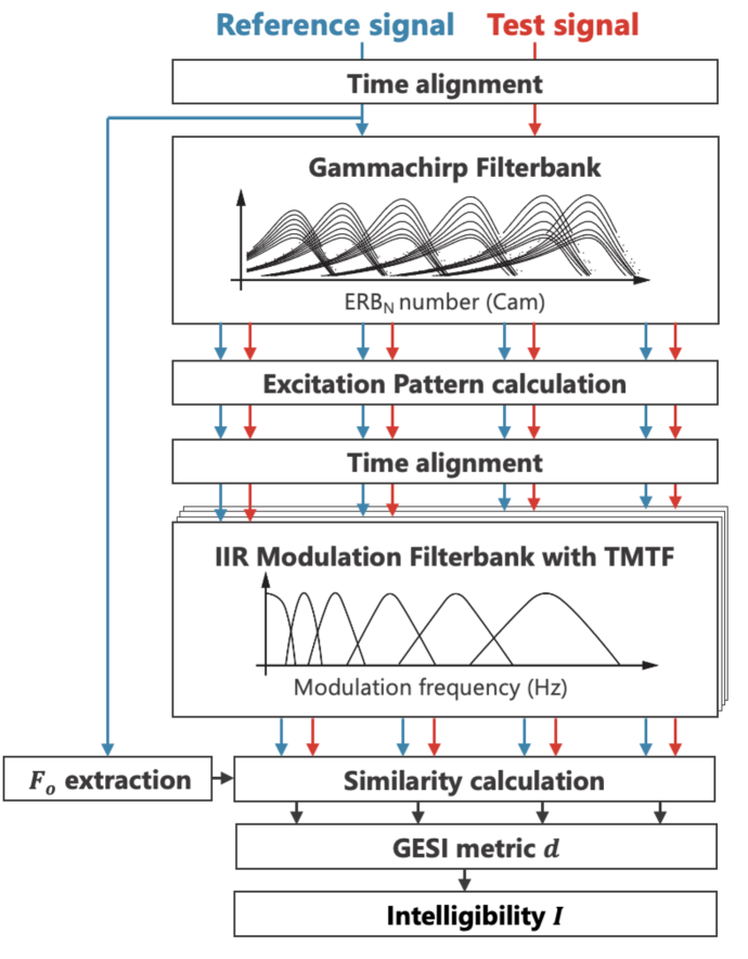
Figure 1 shows the block diagram of GESI. The input sounds to GESI are reference () and test () signals. First, the cross-correlation between them is computed to perform the time alignment of the speech segment. Then, both signals are analyzed with the gammachirp auditory filterbank (GCFB) [Irino & Patterson, 2006, Irino, 2023], which contains the transfer function between the sound field and the cochlea. The output is the Excitation Pattern (EP) sequence with 0.5 ms frame shift, something like an ``auditory'' spectrogram (hereafter referred to as EPgram). The EP is calculated using the cochlear input-output (IO) function with the absolute threshold (AT) set to 0 dB. The noise floor is represented by a Gaussian noise with a root mean squared (RMS) value of 1 for practical calculations.
The reference speech is always analyzed using the GCFB parameters of a typical NH listener, while the test speech is analyzed using parameters that reflect the individual listener's hearing level, that is either normal or with HL. This allows GESI to reflect cochlear HL resulting from dysfunction of active amplification by outer hair cells (OHCs) and passive transduction by inner hair cells (IHCs). The required input parameters are the hearing level represented by an audiogram, and the compression health parameter (), which indicates the degree of health in the compressive IO function of the cochlea [Irino, 2023]. No dysfunction corresponds to and completely damaged function corresponds to . In this study, the hearing level was set to 0 dB and (i.e., NH level) to analyze the reference signal. The individual listener's hearing level and a default value of , a moderate level, were used to analyze the test signal. This is because the value cannot be estimated without extensive psychoacoustical experiments. See A for more details.
Next, the time offset between the EPgrams of the reference and test speech is compensated for each channel of the GCFB. The cross-correlation is computed to find the peak position within the maximum correction range of , and the time alignment is performed accordingly (see section 2.3.1 for details).
After this correction, the EPgrams are analyzed using an infinite impulse response (IIR) version of the modulation frequency filterbank (MFB) used in GEDI [Yamamoto et al., 2018, 2020]. The MFB was first introduced in sEPSM [Jørgensen & Dau, 2011, Jørgensen et al., 2013] and implemented using the Fourier transform. However, the IIR version is more phase sensitive, which may lead to better prediction. The upper limit of the modulation frequency of the MFB was limited to 32 Hz as described in section 2.3.2. In addition, the peak gain of each filter in the MFB was set to the corresponding value of the TMTF [Morimoto et al., 2019] of NH and older adults, as described in section 2.3.3.
The internal index is computed using an extended version of the cosine similarity between the MFB outputs for the reference signal () and the test signal ():
| (1) |
where is the GCFB channel , is the MFB channel , is a time frame number. is a weight value that allows us to handle the level difference between the reference and test sounds. Although is the original definition of cosine similarity, the level difference is normalized to make the evaluation more difficult. See section 2.3.6 for more details. is a weighting function applied to each GCFB channel, as described in section 2.3.4.
The overall similarity index is obtained by weighting and averaging in Eq. 1 by all and .
| (2) |
where is a weighting function applied to each MFB channel. In this study, is used, but is adjustable.
The metric can be converted to word correct score (%) or intelligibility by the sigmoid function used in STOI [Taal et al., 2011] and ESTOI [Jensen & Taal, 2016]. That is:
| (3) |
where and are parameters determined from a subset of the SI scores in the experimental results using the least squares error method. represents the maximum SI specific to the speech dataset used in the experiments. In this study, it was set to 85% based on the SI data of the least familiar words in FW07, i.e., a subset of FW03 [Amano et al., 2009].
Conversion to SI is necessary when calculating the RMS error between the subjective and objective SI. However, this is not necessary to compare the performance of SE algorithms. The metric can be used directly, as is commonly done in much of the literature (e.g., Falk et al., 2015), because the SI score is monotonically related to the metric as defined in Eq. 3.
2.3 Processing in each block of GESI
The processing in each block of GESI is explained with extensions from the original version [Irino et al., 2022, Yamamoto et al., 2023].
2.3.1 Time alignment of EPgram
When listening to speech in a real room environment, reverberation characteristics have a significant impact on speech perception [Steeneken & Houtgast, 1980]. The room impulse response (RIR) that represents these characteristics varies greatly with location and head orientation and is usually unmeasured and unknown. Therefore, it is necessary to consider the effect in the objective metric.
The EPgrams of the dry reference and reverberant test speech have different time delays across the frequency channels. This causes an initial phase difference at the input of the MFB and results in a degradation of the similarity value in Eq. 1. To solve this problem, we introduced a time alignment mechanism in each EPgram channel. The preliminary experiments have shown that the prediction accuracy is improved compared to the previous GESI.
This approach is also inspired by the strobed temporal integration mechanism of the Stabilized Wavelet-Mellin Transform (SWMT), a computational model of speech perception [Irino & Patterson, 2002]. This mechanism synchronizes auditory filterbank outputs in phase. Since the temporal resolution of auditory images in the SWMT is about 30 ms, we set the maximum correction range to . Without this constraint, similarity calculations could be performed between adjacent different phonemes. This could potentially decrease prediction accuracy.
2.3.2 Upper modulation frequency of the MFB
It is also important to note that the RIR reduces the modulation depth of speech sounds at the listener's ear. In fact, the Speech Transmission Index (STI) [Steeneken & Houtgast, 1980] is a pioneering SI metric that reflects this effect in the equation. In the STI, the upper limit of the modulation frequency is 16 Hz. Based on this, the limit in the current GESI has been set at 32 Hz with a small margin.
2.3.3 Introduction of the TMTF into the MFB
Recently, hidden hearing loss [Liberman et al., 2016, Liberman, 2020] has been reported in individuals who have difficulty understanding speech in noisy environments, although the decline in audiogram is not as severe. It is often caused by auditory neuropathy or synaptopathy with a decrease in temporal processing characteristics [Zeng et al., 1999, Narne, 2013]. The SI in older adults with HL may be affected by similar factors, although to a lesser extent. The TMTF is one of the measures used to capture such characteristics. It has been reported that the modulation detection sensitivity in the TMTF is reduced in older adults with HL compared to NH adults [Morimoto et al., 2019]. Therefore, it seems important to include the TMTF in the OIMs. In this study, we introduced the TMTF of individual older adults into GESI and tested the effect as a first attempt in the history of OIM development.
The TMTF measurement was performed using the two-point method [Morimoto et al., 2019] as described in B. This method assumes a first-order low-pass filter (LPF) and estimates the modulation depth threshold ( in dB) at low modulation frequencies and the LPF cutoff frequency ( in Hz). Because the measurement uses broadband noise, it cannot directly reflect the gain or compression characteristics of individual auditory filters. Therefore, for simplicity, we assumed that the low-pass filter gain of the TMTF is equal to the peak gain of the MFB for all GCFB channels as a first-order approximation. The peak gain is then formulated for the NH listener to analyze the reference signal () and for a HL listener to analyze the test signal (),
| (4) | |||||
| (5) |
where is the MFB channel and is the MFB frequency; and are the modulation depth thresholds of the NH and HL listeners, respectively, and and are their cutoff frequencies. The peak gain is usually reduced in the test signal analysis since in many cases. Note that the first MFB filter is an LPF with a cutoff frequency of 1 Hz and we set to maintain the DC modulation level, which is related to the AT.
2.3.4 Weighting function for the GCFB channels
The weighting function for the GCFB channel in Eq. 1 is formulated as the product of two weighting functions, and . is a weighting function designed to reduce the influence of the fundamental frequency (e.g. gender differences) on the phonetic features. represents the efficiency of the GCFB channels above the threshold and is described in the next section.
In the aforementioned SWMT, the Size-Shape Image (SSI) was proposed as a representation of speech features [Irino & Patterson, 2002]. This is a three-dimensional representation in which a two-dimensional image changes over time, allowing an effective representation of speech features independent of . To validate the effectiveness of this representation, an attempt was made to explain psychophysical experimental results related to human size perception [Smith et al., 2005, Matsui et al., 2022]. In the process, a weighting function called ``SSIweight'' was proposed by reducing one dimension of SSI to fit the two-dimensional representation of EPgram. It was shown that the SSIweight could effectively explain the experimental results regardless of whether the speech was male or female [Matsui et al., 2022].
Based on this finding, the previous version of GESI [Irino et al., 2022, Yamamoto et al., 2023] included the SSIweight, where it was set to a fixed value corresponding to the average of male speech. However, this static approach may not adequately account for within-speech variation or differences in between male and female voices. To address this, the current version introduces , a dynamically varying weighting function defined as a function of frame time , formulated as follows.
| (6) |
where represents the peak frequency of the -th channel in the GCFB. denotes the fundamental frequency of the reference speech at frame time , which can be estimated using tools such as the WORLD speech synthesizer [Morise et al., 2016]. However, for certain sounds, such as some consonants where there is no , a small positive value close to zero is assigned. This ensures that the sum of for all is equal to 1. is a constant that determines the boundary between where the weight value gradually increases and where it becomes 1. This comes from the upper limit of the horizontal axis in the two-dimensional SSI in SWMT [Irino & Patterson, 2002].
2.3.5 Weighting function for channel efficiency
Since the reference speech is analyzed using the GCFB parameters of the NH listener, the EP levels in the EPgrams are always above the AT. In contrast, the test speech is analyzed using the parameters that reflect the individual listener's HL. For older listeners with HL, some high frequency channels may have EP levels falling below the AT, making them inaudible.
As age-related HL gradually progresses, individuals may compensate by extracting speech information from the remaining audible regions, potentially increasing overall efficiency. We formulate this effect as a weighting function. Let be the average EP value over all time frames for the -th GCFB channel (total channels). Channels where this value exceeds the AT (i.e., 0 dB) can be considered as contributing to the information extraction. Defining the number of such audible channels as , the weighting function is formulated as follows.
| (7) |
where is a constant representing the efficiency. No information can be obtained from channels where is less than or equal to AT, so the weight is set to 0. On the other hand, for channels with values greater than AT, the weight is set as the efficiency-related weight. If , there is no efficiency improvement and no compensation is made for channel reduction. On the other hand, if , the efficiency is improved by fully compensating for the channel reduction, making it equivalent to using all channels. However, the audible range is limited and may not reach NH levels. The efficiency may depend on factors such as listening effort, concentration, and cognitive processes. Therefore, it may be possible to use to introduce cognitive factors into SI prediction using GESI, which is only a bottom-up process.
In this study, was chosen based on preliminary predictions of subjective SI scores in the current experiment. It was confirmed that clearly led to overestimation and clearly led to underestimation. Additionally, when there was not much difference, but it is believed that optimization can be done depending on the experimental participants and conditions. The effect of variation of other than 0.7 is discussed in section 4.3.
2.3.6 Setting of the parameter
The parameter in Eq. 1 was introduced to correspond to the difference in sound pressure levels between the reference and test signals. An important constraint is that the predicted SI score should be low when the test signal level is significantly lower than the reference signal level. If , the levels of reference and test MFB outputs are equalized, and the above constraint cannot be maintained. Therefore, setting other than 0.5 is essential. In the previous study on SI prediction for both laboratory and crowdsourced experiments [Irino et al., 2022, Yamamoto et al., 2023], was defined as a function of tone-pip test results that roughly provide the information about the sensation level (SL) of test sounds for each listener in the given environment. The experiment in this study was performed in the same quiet laboratory, and the SLs for all listeners were sufficiently above the AT. Therefore, we assumed that accurate predictions could be obtained using a value of similar to that used to predict the SI in the previous laboratory experiment. Thus, we set the value to 0.55.
2.4 OIM for comparison: HASPIw2
The purpose of GESI is to provide information on improvements in SE for older adults with HL. Two important functions are required for such OIMs. First, they must reflect peripheral dysfunctions, including hearing level. Second, they must explicitly represent how the improvement is achieved at the auditory feature level to allow for further improvement. Thus, they must be based on at least a peripheral auditory model. Competitors should have similar functions.
STOI and ESTOI are popular metrics used to evaluate the performance of signal processing. They are simple and effectively used in many SE studies. However, neither metric accounts for individual hearing levels. Recent DNN-based SI models, such as those proposed in the first and second CPC (CPC1 and CPC2) [Barker et al., 2022, 2024], can reflect individual hearing levels. The performance of SI prediction in the competition is excellent. However, it is difficult to understand how the improvements were achieved through signal processing. These models may not provide sufficient information to improve the enhancement process.
HASPI [Kates & Arehart, 2014] and its successors are based on an auditory model and may fulfill the above functions. There are three major versions: the original HASPI [Kates & Arehart, 2014], HASPI version 2 (or HASPIv2) [Kates & Arehart, 2021], and HASPIw2 [Kates, 2023]. The original HASPI [Kates & Arehart, 2014] is simple and produces several internal metrics that are mapped to an SI score via a sigmoid function. But this function differs from Eq. 3 in that it accepts multiple inputs. Because there are no reported preset values for the parameters, it is difficult to use, and stable prediction values cannot be obtained easily. To address this issue, HASPI has been improved and now exists as HASPIv2 and the latest HASPIw2. Furthermore, previous experiments have shown that the original HASPI has lower predictive performance than the previous version of GESI [Irino et al., 2022], so it was not considered a competitor.
Both HASPIv2 and HASPIw2 produce a single SI score calculated by using NN although there are 10 independent internal metrics. It is possible to derive the SI score for the current experiment by assuming the NN output is considered as a single internal metric and transformed into by the sigmoid function in Eq. 3. In practice, this method allowed HASPIv2 to serve as the baseline model in CPC2 [Barker et al., 2024]. Although the internal representations of HASPSIv2 and HASPSIw2 are difficult to interpret due to the NN in the output stage, they are preferable to DNN models because they are more compact.
The NNs are trained on English speech samples from the HINT database [Nilsson et al., 1994] and the IEEE sentence [Rothauser, 1969] with different distortions [Kates & Arehart, 2021, Kates, 2023]. HASPIv2 is tuned for the SI of the entire sentence, which includes the higher-level linguistic information. In this experiment, the accuracy rate is based on individual words, so consistency cannot be ensured, making it unsuitable. As the most recent version tuned for keyword SI, HASPIw2 is expected to outperform HASPIv2 in predicting words. Therefore, HASPIw2 was used as the competitor in the SI prediction of the current experiment.
It would also be important to examine the generalizability of HASPIw2 to other languages and experimental conditions to get an idea of the scope of its application.
3 SI experiments with older adults
The SI experiment with older adults was conducted to evaluate the effects of SE using IRM and the performance of OIMs. In this experiment, we used unfamiliar Japanese words. When using language, it is impossible to avoid cognitive factors that differ from person to person. However, we wanted to conduct an experiment that controlled for these factors as much as possible. GESI is a bottom-up model that does not reflect higher-level knowledge. Prediction accuracy is naturally expected to be low when using sentences that incorporate higher-level contextual information. Conversely, monosyllables are not suitable for predicting SI scores in everyday life. Therefore, we selected words that strike this balance. Nevertheless, words that are easily guessed or completely unfamiliar may result in varying SI scores. Thus, we used words from the familiarity-controlled database.
3.1 Experimental procedure
3.1.1 Speech materials
It is important to minimize cognitive factors such as guessing familiar words in SI experiments used to assess OIMs. There is a Japanese 4 mora word dataset FW07 [Sakamoto et al., 2006], for which familiarity is reasonably well controlled. Note that the Japanese mora is a linguistic unit that generally corresponds to a V (vowel) or CV (consonant-vowel) syllable, with some exceptions. The FW07 is a subset of the FW03 dataset [Amano et al., 2009], whose properties have been well studied and widely used in Japanese SI experiments. It is also possible to exclude sentence-level context. We used the speech words pronounced by a male speaker (`mis') from the minimum familiarity rank data in FW07.
To simulate a realistic listening environment, room reverberation was applied to the speech sounds. Babble noise was then added to control the SNR. The RIR was obtained from the Aachen database [Jeub et al., 2009]. The target speech was convolved with the RIR for 2 m distance in an office room. The babble noise was convolved with the RIRs for 1 m and 3 m separately and added together to have more diffuse characteristics. The signal-to-noise ratio (SNR) was set between -6 dB and 12 dB, increasing in 6 dB steps. The masking effect should be maximized, since the babble noise was created by overlapping and adding a large number of randomly selected word sounds from the FW03 dataset. This condition is referred to as the unprocessed (hereafter ``Unpro'') because no SE algorithm was applied.
We also prepared the word sounds processed by the SE using IRM to evaluate its effectiveness on SI for older adults. The use of IRM has been proposed to provide oracle data for training the DNN-based SE algorithms [Wang et al., 2014], and its procedure is briefly described in C. The ``Unpro'' sounds of the other words were processed with the IRM, and the condition is referred to as ``IRM''. Since the sound clarity processed by a real SE algorithm should be lower than that of the IRM algorithm, the SI values in the practical situation are expected to be larger than those of ``Unpro'', but smaller than those of ``IRM''.
The IRM-enhanced speech was found to be clearer when processed at a sampling frequency of 16 kHz compared to 48 kHz. Based on this, all of the signal processing described above was performed at 16 kHz and then upsampled to 48 kHz to ensure reliable playback on the experimental website [Yamamoto et al., 2021].
3.1.2 Data collection
Each of the eight conditions, consisting of two signal processing conditions (``Unpro'' and ``IRM'') and four SNR conditions, was assigned a set of 20 words from FW07. Thus, the total number of words was 160 (= 20 2 4), and each participant listened to a different list of words. The sounds were played on the web-based GUI system [Yamamoto et al., 2021]. 160 words were presented in 16 sessions of 10 words each. A word was played and 6 seconds were given to respond, then the next word was played. The 6-second response time was longer than the 4-second response time in the previous experiments with NH participants to allow more time to respond. Participants listened to the words and wrote them down on a response sheet during this 6-second period. Even if they did not hear the word completely, they were instructed to guess and respond. After all listening sessions were completed, the answered words were reviewed and entered into the GUI system by the experimenters to avoid unfamiliar keyboard input for the participants. From this data, the correct rates for word, phoneme, and mora, as well as the confusion matrix, were calculated.
Experimental details were explained with documentation, and informed consent was obtained in advance. The experiment was approved by the ethics committee of Wakayama University (Nos. 2015-3, Rei01-01-4J, and Rei02-02-1J).
3.1.3 Acoustic condition
The participants were seated in a sound-attenuated room (YAMAHA AVITECS) with a background noise level of approximately 26.2 dB in . The sounds were presented diotically through a DA-converter (SONY, Walkman 2018 model NW-A55) connected to a computer (Apple, Mac mini) via headphones (SONY, MDR-1AM2). The sound pressure level (SPL) of the unprocessed sounds was 63 dB in by default, which was the same level as the calibration tone measured with an artificial ear (Brüel & Kjær, Type 4153), a microphone (Brüel & Kjær, Type 4192), and a sound level meter (Brüel & Kjær, Type 2250-L). However, four participants reported that the sound was either too loud or too quiet to hear, so the SPL was adjusted to a comfortable level for each participant (62.5, 65, 68, or 70 dB).
3.1.4 Participants and hearing characteristics
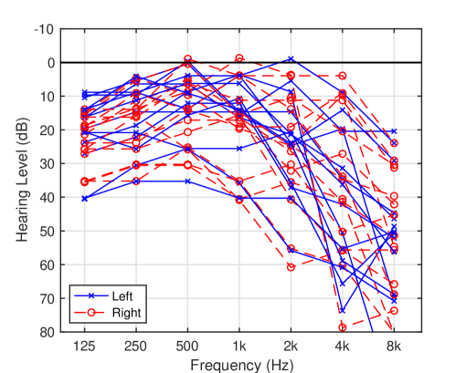
The participants in the experiment were 16 people between the ages of 62 and 81 who were recruited through the Senior Human Resources Center in Wakayama. Their native language is Japanese. The audiograms obtained by pure-tone audiometry are shown in Fig. 2 for 15 participants (one of them was excluded as described shortly).
The hearing levels of the participants varied, but most of them showed typical signs of age-related HL, which is a decrease in hearing levels at 8 kHz. We calculated the average hearing level from 500 Hz to 4000 Hz for each ear, and the ear with the lower value was considered the better ear. Average hearing levels for the better ear ranged from 8.8 to 43.8 dB. Nine participants had levels less than 22 dB, which could be considered NH.
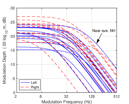
The TMTF was also measured using the two-point method as described in B [Morimoto et al., 2019]. The results are used for SI prediction in GESI (see section 2.3.3). Note that one participant was unable to perform the TMTF experiment due to difficulty following the procedure and was excluded from the analysis. Therefore, the results reported here are based on 15 participants.
The TMTF curves for each ear are shown in Fig. 2. The sensitivity of modulation detection is higher when the curves are at higher positions in the figure. The thresholds of the modulation depth at the low frequency () were in the range from -15 to -27 dB. The cutoff frequencies () also vary widely. The blue line indicated by the arrow is close to the TMTF curve for the average NH listener ( -23 dB and 128 Hz, see B). Because many curves lie below this line, the modulation sensitivity of the older participants is generally lower than that of the NH listener.
3.2 Results
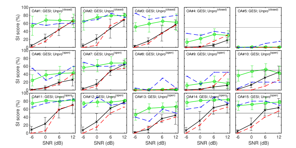
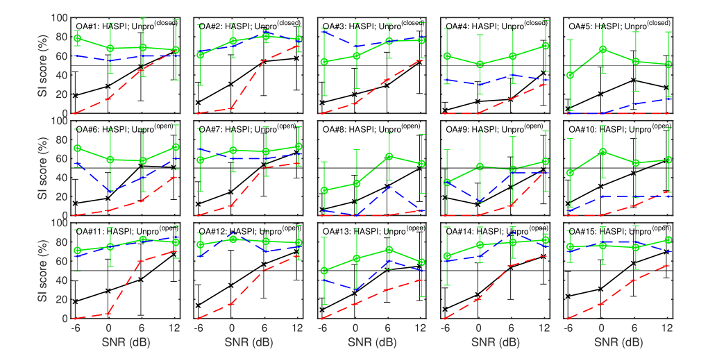
We calculated SI as the percentage of 4 mora words that the participants answered correctly. Their results are shown as dashed lines in Fig. 3 and 3 along with the predictions of GESI and HASPIw2 described in the next section. There are 15 panels each, with participant IDs assigned from to in order of participation. There are large individual differences in SI between participants, which may be due to differences in hearing level, temporal characteristics, and cognitive factors. The results of the ``Unpro'' condition (red dashed line) show that the SI score improves with increasing SNR. In contrast, the results of the ``IRM'' condition (blue dashed line) show that the SI score does not change much depending on the SNR. This indicates that the effect of the IRM-based SE is more pronounced at lower SNRs. The SI scores for sounds enhanced by a practical SE algorithm are expected to lie between the two SI curves. These subjective SI scores are the target of the OIM predictions.
4 Prediction by OIMs
The goal of OIMs is to accurately predict the SI of individual listeners and the effect of SE. This study investigated whether the subjective SI scores in Figs. 3 and 3 could be predicted using GESI and HASPIw2. In addition, statistical analysis was performed to confirm the results.
4.1 Condition
The hearing levels of the better ear in Fig. 2 were used for both GESI and HASPIw2. GESI requires compression health () to specify the slope of the cochlear IO function in GCFB, while HASPIw2 automatically sets the parameter for the similar function. The initial value of was set to a moderate value of 0.5 for all participants as described in A. GESI can also include the individual TMTF shown in Fig. 2, which has been set to that of the better ear defined in the hearing level.
It is necessary to estimate the sigmoid parameters and in Eq. 3 in order to convert the internal metric to the SI score in this experiment. In Figs. 3 and 3, the subjective SI scores of the ``Unpro'' condition for the first 5 participants ( to ) were used for this estimation. 20 words were assigned for each participant and each of the 4 SNR conditions (denoted by ``''). The values for these 20 words were calculated and averaged to obtain the average metric . This was converted to a predicted SI score using the sigmoid in Eq. 3. The values of and were estimated by the least-squares method to minimize the error between and the subjective SI score for the five participants and 4 SNR conditions. SI scores for 20 words were then predicted using these and values for all participants, SNR conditions, and signal processing conditions (``Unpro'' and ``IRM''). Therefore, the SI scores in ``'' and ``IRM'' were predicted in the open condition.
4.2 Prediction results
The prediction results for the 15 participants are presented as mean and standard deviation for 20 words with error bars in Figs. 3 for GESI and 3 for HASPIw2. The ``'' shows the conditions under which the ``Unpro'' SI scores were used to determine the parameters and of the sigmoid function in Eq. 3. The ``'' shows the case where the prediction was performed with the open condition using the and derived above. Note that the prediction for the ``IRM'' sound was always evaluated with the open condition.
GESI generally predicted quite well for all participants for both ``Unpro'' and ``IRM''. The major differences are only noticeable in the cases of and for underestimation and for overestimation. In contrast, the predictions of HASPIw2 were not as good as those of GESI. In particular, the standard deviation of 20 words is much larger than that of GESI. The average SI scores for , , , , and are much more overestimated than those in GESI. In the case of , it should have made better predictions even for HASPIw2 because the subjective SI score was used to determine the sigmoid parameters and as in ``'', but it did not. This is probably because the metric value estimated by HASPIw2 is highly variable across words and its mean is always well above zero. As described in section 2.4, HASPIw2 uses the NN trained by English keywords. The current results suggest that the generalization ability to this experiment using Japanese words is not very high.
4.3 Effect of variation
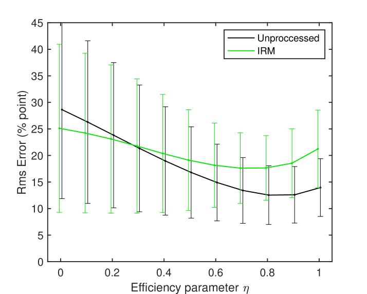
The above results were calculated using an efficiency coefficient of 0.7, which was determined in a preliminary study. The validity of this value was not demonstrated. Therefore, we investigated the extent to which affects the error. Figure 4 shows the RMS error of individual words when is varied from 0 to 1 in increments of 0.1. The open and closed conditions were the same as in the above prediction shown in Figure 3.
The curves changed gradually, with no unusual increases or decreases that would suggest overfitting. In the ``Unpro'' condition, the minimum value was achieved at , while in the ``IRM'' condition, the minimum value was achieved at . Since ``Unpro'' includes both closed and open conditions, whereas ``IRM'' only includes open conditions, its overall RMS error value is lower than that of ``IRM''. The standard deviation is approximately 6% at or , which is lower than for the other values. This indicates reduced variability in predictions. Therefore, a value of 0.7 seems to be reasonable for the current prediction.
In this way, GESI's interpretable parameter can be determined through learning using data from a large number of listeners. However, it is thought that adjusting the value of for individual listeners is more effective. This value is thought to allow for the simple introduction of factors that cannot be expressed by the bottom-up model of GESI, such as the influence of the mental lexicon, listening effort, and cognitive factors, into a single value. However, this is beyond the scope of this paper, and further research is awaited.
4.4 Statistical analysis
Statistical analysis was performed to confirm whether the SI prediction described above is stable and generalizable across different combinations of open and closed sets in GESI and HASPIw2.
For this purpose, different 5 participants were randomly selected to determine the sigmoid parameters and from their SI scores of the ``Unpro'' condition, and all SI scores were predicted as described above. This prediction was repeated 9 times for a total of 10 results. Furthermore, this procedure was also performed when the TMTF was not introduced in GESI, by substituting the HL parameters for the NH parameters in Eq. 5, i.e. . Then the RMS errors were computed in two ways described below and accumulated for three processing conditions of ``'', ``'' and ``IRM''.
4.4.1 Prediction error of individual word
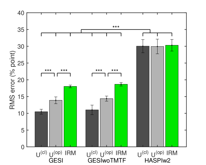
The RMS values between the predicted SI scores of individual words and the subjective SI score were calculated for each participant and experimental condition. Figure 5 shows the mean RMS errors and 95% confidence intervals. The mean RMS errors of ``'', ``'', and ``IRM'' are 10.5, 13.9, and 18.0 % points in GESI on the 3 leftmost bars. This prediction in ``'' is more difficult than in ``'', as expected. The prediction in ``IRM'' is the most difficult. However, it is not easy to determine whether an error of 18% points is so large that it cannot be used practically, especially considering that the standard deviation of the subjective SI scores in the IRM condition was also quite large. The mean RMS errors in HASPIw2 are about 30% points regardless of the processing condition and much larger than the maximum in GESI. The results reflect that the standard deviations of the predicted SI scores are much larger in HASPIw2 than in GESI, as shown in Fig. 3. The mean RMS errors in GESI with the TMTF (3 leftmost bars) and without the TMTF (3 middle bars) are about the same.
A three-way analysis of variance (ANOVA) was performed on the following factors: OIM (GESI with and without the TMTF, and HASPIw2), processing condition, and repetition of prediction. The main effects of the OIM, processing, and repetition were significant (). The interactions between the factors were also significant (), except for the interaction between processing and repetition (). Tukey's HSD multiple comparison tests revealed significant differences between GESI and HASPIw2 () for all processing conditions. For GESI, there are significant differences between the three processing conditions. However, there is no significant difference within the same processing condition between with and without the TMTF.
4.4.2 Prediction error in mean across words
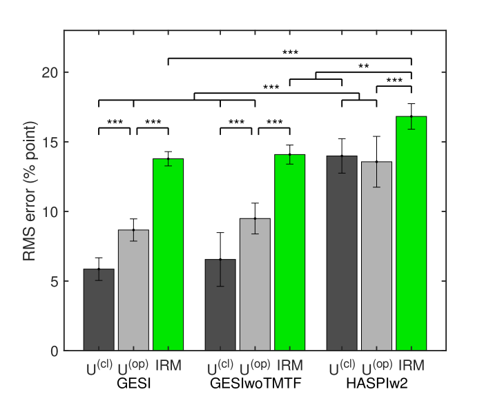
The above evaluation may be too strict for HASPIw2 with the larger standard deviation across words. The case where the average of multiple predictions can be used as a metric was also evaluated to relax the condition. The RMS values between the SI score derived from the metric averaged over all 20 words and the subjective SI score were calculated for each participant and experimental condition. Figure 5 shows the results. A three-way ANOVA showed results similar to those in the above section. The difference between GESI and HASPIw2 is smaller than it appears in Fig. 5. However, Tukey's HSD tests revealed significant differences between the two under the same processing conditions ( and ). The difference is expected to increase as the number of words used for averaging decreases. This implies that GESI is still better than HASPIw2 in this evaluation.
5 Discussion
5.1 Limitations and Potential of GESI
GESI was developed to evaluate the effectiveness of signal processing techniques, such as SE and noise suppression, for older individuals with HL. GESI is a bottom-up model configured with only a few explicitly defined parameters, in order to clarify the improved internal representation by signal processing. The values of the sigmoid parameters and in Eq. 3 depend on the evaluation material and conditions. They require a few matched data sets of signal and subjective SI scores. However, these two parameters are unnecessary when GESI is used for performance comparisons.
This feature also highlights a fundamental limitation of GESI. The current version of GESI does not model the factors involved in central auditory and cognitive processes. Therefore, it is impossible to differentiate the SI scores of listeners with similar hearing level profiles but different central and cognitive dysfunctions or improvements. Furthermore, only two parameters, and , connect the bottom-up metric and the SI score. These are insufficient for incorporating all the complex, higher-order information that depends on listeners and situations. This differs from recent DNN-based models, which can make more accurate predictions with a large amount of training data.
Nevertheless, when parameters and are determined using a part of individual's SI scores, it is possible to fairly evaluate the effectiveness of signal processing for that individual, as demonstrated under the IRM conditions shown in Fig. 3. This may provide valuable information to improve signal processing. This is an important application of GESI.
GESI has another usage. Depending on the hearing level setting, GESI can predict SI scores for both older adults with HL and young NH individuals. Additionally, GESI only models bottom-up processes. These properties could be used to distinguish between peripheral and central factors contributing to the SI score [Yamamoto et al., 2025]. First, the parameters and in the sigmoid are estimated using the SI scores of multiple young NHs who are expected to have normal cognitive function. Next, the hearing level of a specific older adult is set and their SI scores are predicted based on these values of and . If the predicted SI score is worse than the score obtained in the subjective experiment, it can be estimated that this older adult has dysfunction in their higher-level processing or cognitive factors. Conversely, a higher predicted SI could suggest greater efficiency in using the mental lexicon or in other higher-level processing in response to gradually declining peripheral hearing level. This method could help to identify the cause of HL.
5.2 Introduction of the TMTF
In this study, we tried to incorporate the TMTF of individual listeners into GESI. However, as shown in 5, there was no difference between the GESI results with and without the TMTF. There are two possible reasons for this.
First, the TMTFs of the older participants were not as poor as those of the neuropathy patients, whose were greater than -10 dB on average [Narne, 2013]. As a result, the effect of the TMTF may not have been large enough to be observed. However, it remains difficult to conclude whether this is a reasonable explanation.
The second reason is a technical issue that should be improved. The TMTF introduction method described in section 2.3.3 was imprecise. The TMTF measurement described in B was performed with broadband noise to simplify and expedite the process. Then, the estimated low-pass characteristics were uniformly reflected in the peak gain of the MFB, regardless of the frequencies in the GCFB channels. This may have negatively impacted the results. The temporal characteristics may differ from channel to channel. Furthermore, modulation differences can only be detected at low frequencies within the audible range for older adults with age-related HL. Therefore, the measured results may not reflect the temporal characteristics of high frequencies. To avoid this issue, the TMTFs should be measured at each audiometric frequency. If a sinusoid is used for simplicity, the response curve will not become a simple low-pass filter because of the sideband components produced by the modulation [Kohlrausch et al., 2000]. However, this does not affect the current version of GESI since the minimum modulation depth remains nearly constant below 32 Hz. Alternatively, bandpass noise could also be used for the measurement.
The method of introducing the TMTF into the MFB should also be considered more carefully. In this study, the measured TMTF was applied directly to the peak gain of the MFB. However, compensation may be necessary because the auditory filter has compressive characteristics. It is important to take these issues seriously and incorporate them into the design of OIMs.
5.3 Generalization ability
The results shown in section 4 suggest that GESI is more advantageous than HASPIw2 in predicting current experimental results. Therefore, HASPIw2 is not sufficiently capable of generalizing to Japanese word SI prediction. It may be possible to train the NNs in HASPIw2 using compatible Japanese word data to improve performance. However, with such a strategy, the training would likely need to be tailored for each language, experimental condition, and listening condition.
Conversely, we also examined whether GESI could generalize to English SI prediction. Here, we compared HASPIv2 and GESI using CPC2 data [Barker et al., 2024]. The rationale for using CPC2 data and the comparison with HASPIv2, the evaluation method, and the results are presented in detail in D. It was difficult to conduct a comparison as rigorous as the prediction presented here because of missing information of the SPL in the CPC2 data. However, the evaluation was designed to be fair by aligning the conditions as much as possible.
The results of D show that the RMS errors in the open test were not significantly different between HASPIv2 and GESI. In theory, GESI is not superior to HASPIv2 for the CPC2 task because GESI cannot represent higher-order linguistic knowledge, whereas HASPIv2 can. Nevertheless, similar performance was achieved, and GESI is reasonably applicable for predicting English SI with word segmentation.
It is also worth considering the complexity of the models by examining the necessary parameters. Both models use the sigmoid parameters, and . HASPIv2 additionally uses NNs with ten input units (plus one constant unit), four hidden units (plus one constant unit), one output unit. This configuration yields a total of more than 44 uninterpretable weight parameters. In contrast, GESI uses only two explicitly defined parameters and . This suggests that the same level of performance could be achieved with far fewer parameters. Following Occam's razor principle [McFadden, 2021], GESI is clearly simpler and more efficient. Furthermore, this result provides valuable insight into how peripheral processing affects SI.
6 Conclusion
In this study, a new OIM GESI was extended to predict subjective SI scores in older adults. To assess performance, an SI experiment with familiarity-controlled words was conducted with older adults of different HLs. The TMTF was also measured to see if the temporal response characteristics could be reflected in the prediction. The SI prediction of speech-in-noise and its IRM-enhanced sounds was compared with HASPIw2, which was developed for keyword SI prediction. The results showed that GESI was more accurate than HASPIw2 in the current experiment. GESI is a bottom-up model based on psychoacoustic knowledge from the peripheral to the central auditory system, with explicitly defined parameters. In contrast, HASPIw2 uses such a bottom-up model with NNs that contain many noninterpretable weight parameters. The results suggested that its ability to generalize to Japanese word-level SI, i.e., outside the training domain, was limited. On the other hand, GESI was found to predict English sentence-level SI at a level similar to that of HASPIv2 when using simple word segmentation as described in D. Introducing the TMTF into the GESI algorithm had no significant effect. This suggests that more effective measurement and implementation methods are needed to incorporate temporal response characteristics. GESI is available from our GitHub repository [AMLAB GitHub, 2019].
Acknowledgments
This research was supported by JSPS KAKENHI: Grant Numbers JP21H03468, JP21K19794,and JP24K02961. The author thanks Takashi Morimoto for the TMTF measurement software and Sota Bano for experimental assistance.
Declaration of generative AI and AI-assisted technologies in the writing process
During the preparation of this work the authors used DeepL Write and DeepL Translate in order to improve language and readability. After using this service, the authors reviewed and edited the content as needed and take full responsibility for the content of the publication.
References
- Akeroyd et al. [2023] Akeroyd, M. A., Bailey, W., Barker, J., Cox, T. J., Culling, J. F., Graetzer, S., Naylor, G., Podwińska, Z., & Tu, Z. (2023). The 2nd clarity enhancement challenge for hearing aid speech intelligibility enhancement: Overview and outcomes. In ICASSP 2023-2023 IEEE International Conference on Acoustics, Speech and Signal Processing (ICASSP) (pp. 1–5). IEEE.
- Amano et al. [2009] Amano, S., Sakamoto, S., Kondo, T., & Suzuki, Y. (2009). Development of familiarity-controlled word lists 2003 (FW03) to assess spoken-word intelligibility in Japanese. Speech Commun., 51, 76–82. doi:10.1016/j.specom.2008.07.002.
- AMLAB GitHub [2019] AMLAB GitHub (2019). https://github.com/amlab-wakayama/. (Last: 12 Aug. 2025).
- Anovum [2022] Anovum (2022). JapanTrack 2022 (Japan Hearing Aid Manufacturers Association ). URL: https://hochouki.com/files/2023_JAPAN_Trak_2022_report.pdf.
- Barker et al. [2024] Barker, J., Akeroyd, M., Bailey, W., Cox, T. J., Culling, J. F., Firth, J., Graetzer, S., & Naylor, G. (2024). The 2nd clarity prediction challenge: A machine learning challenge for hearing aid intelligibility prediction. In Proc. ICASSP 2024. doi:10.1109/ICASSP48485.2024.10446441.
- Barker et al. [2022] Barker, J., Akeroyd, M., Cox, T. J., Culling, J. F., Firth, J., Graetzer, S., Griffiths, H., Harris, L., Naylor, G., Podwinska, Z. et al. (2022). The 1st clarity prediction challenge: A machine learning challenge for hearing aid intelligibility prediction. In Proc. Interspeech 2022. doi:10.21437/Interspeech.2022-10821.
- BNC Consortium [2007] BNC Consortium (2007). British national corpus xml edition, oxford text archive core collection (2007). URL: http://www.natcorp.ox.ac.uk/ last: 10 Aug 2025.
- Braza et al. [2022] Braza, M. D., Porter, H. L., Buss, E., Calandruccio, L., McCreery, R. W., & Leibold, L. J. (2022). Effects of word familiarity and receptive vocabulary size on speech-in-noise recognition among young adults with normal hearing. Plos one, 17, e0264581.
- Falk et al. [2015] Falk, T. H., Parsa, V., Santos, J. F., Arehart, K., Hazrati, O., Huber, R., Kates, J. M., & Scollie, S. (2015). Objective quality and intelligibility prediction for users of assistive listening devices: Advantages and limitations of existing tools. IEEE Signal Processing Magazine, 32, 114–124. doi:10.1109/MSP.2014.2358871.
- Graetzer et al. [2022] Graetzer, S., Akeroyd, M. A., Barker, J., Cox, T. J., Culling, J. F., Naylor, G., Porter, E., & Viveros-Mu~noz, R. (2022). Dataset of british english speech recordings for psychoacoustics and speech processing research: The clarity speech corpus. Data in brief, 41, 107951.
- Huckvale & Hilkhuysen [2022] Huckvale, M., & Hilkhuysen, G. (2022). ELO-SPHERES intelligibility prediction model for the Clarity Prediction Challenge 2022. In Proc. Interspeech 2022. doi:10.21437/Interspeech.2022-10521.
- Irino [2023] Irino, T. (2023). Hearing impairment simulator based on auditory excitation pattern playback: WHIS. IEEE Access, 11, 78419–78430. doi:10.1109/ACCESS.2023.3298673.
- Irino et al. [2024] Irino, T., Doan, S., & Ishikawa, M. (2024). Signal processing algorithm effective for sound quality of hearing loss simulators. In Proc. Interspeech 2024 (pp. 882–886). doi:10.21437/Interspeech.2024-111.
- Irino & Patterson [2002] Irino, T., & Patterson, R. D. (2002). Segregating information about the size and shape of the vocal tract using a time-domain auditory model: The stabilised wavelet-Mellin transform. Speech Commun., 36, 181–203. doi:10.1016/S0167-6393(00)00085-6.
- Irino & Patterson [2006] Irino, T., & Patterson, R. D. (2006). A dynamic compressive gammachirp auditory filterbank. IEEE Trans. Audio Speech Lang. Process., 14, 2222–2232. doi:10.1109/TASL.2006.874669.
- Irino et al. [2022] Irino, T., Tamaru, H., & Yamamoto, A. (2022). Speech intelligibility of simulated hearing loss sounds and its prediction using the Gammachirp Envelope Similarity Index (GESI). In Proc. Interspeech 2022 (pp. 3929–3933). doi:10.21437/Interspeech.2022-211.
- Irino et al. [2023] Irino, T., Yokota, K., & Patterson, R. D. (2023). Improving auditory filter estimation by incorporating absolute threshold and a level-dependent internal noise. Trends in Hearing, 27. doi:10.1177/23312165231209750.
- Jensen & Taal [2016] Jensen, J., & Taal, C. H. (2016). An Algorithm for Predicting the Intelligibility of Speech Masked by Modulated Noise Maskers. IEEE/ACM Trans. ASLP, 24, 2009–2022. doi:10.1109/TASLP.2016.2585878.
- Jeub et al. [2009] Jeub, M., Schafer, M., & Vary, P. (2009). A binaural room impulse response database for the evaluation of dereverberation algorithms. In 2009 16th international conference on digital signal processing (pp. 1–5). IEEE. doi:10.1109/ICDSP.2009.5201259.
- Jørgensen & Dau [2011] Jørgensen, S., & Dau, T. (2011). Predicting speech intelligibility based on the signal-to-noise envelope power ratio after modulation-frequency selective processing. J. Acoust. Soc. Am., 130, 1475–1487. doi:10.1121/1.3621502.
- Jørgensen et al. [2013] Jørgensen, S., Ewert, S. D., & Dau, T. (2013). A multi-resolution envelope-power based model for speech intelligibility. J. Acoust. Soc. Am., 134, 436–446. doi:10.1121/1.4807563.
- Kamo et al. [2022] Kamo, N., Arai, K., Ogawa, A., Araki, S., Nakatani, T., Kinoshita, K., Delcroix, M., Ochiai, T., & Irino, T. (2022). Conformer-based fusion of text, audio, and listener characteristics for predicting speech intelligibility of hearing aid users. In Proc. The 2nd Clarity Workshop on Machine Learning Challenges for Hearing Aids (Clarity-2022).
- Kates [2023] Kates, J. M. (2023). Extending the hearing-aid speech perception index (haspi): Keywords, sentences, and context. J. Acoust. Soc. Am., 153, 1662–1673. doi:10.1121/10.0017546.
- Kates & Arehart [2014] Kates, J. M., & Arehart, K. H. (2014). The hearing-aid speech perception index (HASPI). Speech Commun., 65, 75–93. doi:10.1016/j.specom.2014.06.002.
- Kates & Arehart [2021] Kates, J. M., & Arehart, K. H. (2021). The hearing-aid speech perception index (HASPI) version 2. Speech Commun., 131, 35–46. doi:10.1016/j.specom.2020.05.001.
- Kohlrausch et al. [2000] Kohlrausch, A., Fassel, R., & Dau, T. (2000). The influence of carrier level and frequency on modulation and beat-detection thresholds for sinusoidal carriers. J. Acoust. Soc. Am., 108, 723–734. doi:10.1121/1.429605.
- Kohlrausch et al. [1997] Kohlrausch, A., Fassel, R., Van Der Heijden, M., Kortekaas, R., Van De Par, S., Oxenham, A. J., & Püschel, D. (1997). Detection of tones in low-noise noise: Further evidence for the role of envelope fluctuations. Acta Acustica united with Acustica, 83, 659–669.
- Kučera & Francis [1967] Kučera, H., & Francis, W. (1967). Computational analysis of present-day American English. Brown University Press.
- Levitt [1971] Levitt, H. (1971). Transformed up-down methods in psychoacoustics. J. Acoust. Soc. Am., 49, 467–477. doi:10.1121/1.1912375.
- Liberman [2020] Liberman, M. C. (2020). Hidden hearing loss: Primary neural degeneration in the noise-damaged and aging cochlea. Acoustical Science and Technology, 41, 59–62. doi:10.1250/ast.41.59.
- Liberman et al. [2016] Liberman, M. C., Epstein, M. J., Cleveland, S. S., Wang, H., & Maison, S. F. (2016). Toward a differential diagnosis of hidden hearing loss in humans. PLoS ONE, 11, 1–15. doi:10.1371/journal.pone.0162726.
- Livingston et al. [2024] Livingston, G., Huntley, J., Liu, K. Y., Costafreda, S. G., Selbæk, G., Alladi, S., Ames, D., Banerjee, S., Burns, A., Brayne, C., Fox, N. C., Ferri, C. P., Gitlin, L. N., Howard, R., Kales, H. C., Mika, K., Larson, E. B., Nakasujja, N., Rockwood, K., Samus, Q., Shirai, K., Singh-Manoux, A., Schneider, L. S., Walsh, S., Yao, Y., Sommerlad, A., & Mukadam, N. (2024). Dementia prevention, intervention, and care: 2024 report of the lancet standing commission. The Lancet, 404, 572–628. doi:10.1016/S0140-6736(24)01296-0.
- Loizou [2013] Loizou, P. C. (2013). Speech Enhancement: Theory and Practice. (2nd ed.). CRC Press. URL: https://www.crcpress.com/Speech-Enhancement-Theory-and-Practice-Second-Edition/Loizou/p/book/9781138075573.
- Lopez-Poveda et al. [2005] Lopez-Poveda, E. A., Plack, C. J., Meddis, R., & Blanco, J. L. (2005). Cochlear compression in listeners with moderate sensorineural hearing loss. Hearing research, 205, 172–183.
- Matsui et al. [2022] Matsui, T., Irino, T., Uemura, R., Yamamoto, K., Kawahara, H., & Patterson, R. D. (2022). Modelling speaker-size discrimination with voiced and unvoiced speech sounds based on the effect of spectral lift. Speech Commun., 136, 23–41. doi:10.1016/j.specom.2021.10.006.
- McFadden [2021] McFadden, J. (2021). Life is Simple: How Occam's Razor Set Science Free and Shapes the Universe. Basic Books.
- Moore & Glasberg [1997] Moore, B. C., & Glasberg, B. R. (1997). A model of loudness perception applied to cochlear hearing loss. Auditory neuroscience, 3, 289–311.
- Moore [2013] Moore, B. C. J. (2013). An Introduction to the Psychology of Hearing. (6th ed.). Brill.
- Moore et al. [1997] Moore, B. C. J., Glasberg, B. R., & Baer, T. (1997). A model for the prediction of thresholds, loudness, and partial loudness. J. Audio Eng. Soc., 45, 224–240.
- Morimoto et al. [2019] Morimoto, T., Irino, T., Harada, K., Nakaichi, T., Okamoto, Y., Kanno, A., Kanzaki, S., & Ogawa, K. (2019). Two-point method for measuring the temporal modulation transfer function. Ear and Hearing, 40, 55–62. doi:10.1097/AUD.0000000000000590.
- Morise et al. [2016] Morise, M., Yokomori, F., & Ozawa, K. (2016). WORLD: a vocoder-based high-quality speech synthesis system for real-time applications. IEICE Trans Info. Sys., 99, 1877–1884. doi:10.1587/transinf.2015EDP7457.
- Narne [2013] Narne, V. K. (2013). Temporal processing and speech perception in noise by listeners with auditory neuropathy. PLoS One, 8, e55995. doi:10.1371/journal.pone.0055995.
- Nelson et al. [2001] Nelson, D. A., Schroder, A. C., & Wojtczak, M. (2001). A new procedure for measuring peripheral compression in normal-hearing and hearing-impaired listeners. J. Acoust. Soc. Am., 110, 2045–2064.
- Nilsson et al. [1994] Nilsson, M., Soli, S. D., & Sullivan, J. A. (1994). Development of the Hearing in Noise Test for the measurement of speech reception thresholds in quiet and in noise. J. Acoust. Soc. Am., 95, 1085–1099. doi:10.1121/1.408469.
- Nusbaum et al. [1984] Nusbaum, H. C., Pisoni, D. B., & Davis, C. K. (1984). Sizing up the hoosier mental lexicon. Research on spoken language processing report, 10, 357–376.
- Patterson et al. [2003] Patterson, R. D., Unoki, M., & Irino, T. (2003). Extending the domain of center frequencies for the compressive gammachirp auditory filter. J. Acoust. Soc. Am., 114, 1529–1542. doi:10.1121/1.1600720.
- Pumplin [1985] Pumplin, J. (1985). Low-noise noise. J. Acoust. Soc. Am., 78, 100–104. doi:10.1121/1.392571.
- Radford et al. [2023] Radford, A., Kim, J. W., Xu, T., Brockman, G., McLeavey, C., & Sutskever, I. (2023). Robust speech recognition via large-scale weak supervision. In Proceedings of the 40th International Conference on Machine Learning. doi:10.5555/3618408.3619590.
- Rothauser [1969] Rothauser, E. H. (1969). IEEE recommended practice for speech quality measurements. IEEE Transactions on Audio and Electroacoustics, 17, 225–246. doi:10.1109/TAU.1969.1162058.
- Sakamoto et al. [2006] Sakamoto, S., Yoshikawa, T., Amano, S., Suzuki, Y., & Kondo, T. (2006). New 20-word lists for word intelligibility test in japanese. In Proc. Interspeech 2006 - ICSLP (pp. 2158–2161). doi:10.21437/Interspeech.2006-561.
- Schlittenlacher & Moore [2020] Schlittenlacher, J., & Moore, B. C. (2020). Fast estimation of equal-loudness contours using bayesian active learning and direct scaling. Acoustical Science and Technology, 41, 358–360.
- Smith et al. [2005] Smith, D. R., Patterson, R. D., Turner, R., Kawahara, H., & Irino, T. (2005). The processing and perception of size information in speech sounds. J. Acoust. Soc. Am., 117, 305–318. doi:10.1121/1.1828637.
- Steeneken & Houtgast [1980] Steeneken, H. J. M., & Houtgast, T. (1980). A physical method for measuring speech-transmission quality. J. Acoust. Soc. Am., 67, 318–326. doi:10.1121/1.384464.
- Taal et al. [2011] Taal, C. H., Hendriks, R. C., Heusdens, R., & Jensen, J. (2011). An algorithm for intelligibility prediction of time-frequency weighted noisy speech. IEEE Tran. ASLP, 19, 2125–2136. doi:10.1109/TASL.2011.2114881.
- Tu et al. [2022] Tu, Z., Ma, N., & Barker, J. (2022). Exploiting hidden representations from a DNN-based speech recogniser for speech intelligibility prediction in hearing-impaired listeners. arXiv preprint arXiv:2204.04287, . doi:10.48550/arXiv.2204.04287.
- Van Kuyk et al. [2018] Van Kuyk, S., Kleijn, W. B., & Hendriks, R. C. (2018). An evaluation of intrusive instrumental intelligibility metrics. IEEE/ACM Transactions on Audio, Speech, and Language Processing, 26, 2153–2166. doi:10.1109/TASLP.2018.2856374.
- Viemeister [1979] Viemeister, N. F. (1979). Temporal modulation transfer functions based upon modulation thresholds. J. Acoust. Soc. Am., 66, 1364–1380. doi:10.1121/1.383531.
- Wang et al. [2014] Wang, Y., Narayanan, A., & Wang, D. (2014). On training targets for supervised speech separation. IEEE/ACM transactions on audio, speech, and language processing, 22, 1849–1858. doi:DOI:10.1109/TASLP.2014.2352935.
- Yamamoto et al. [2021] Yamamoto, A., Irino, T., Arai, K., Araki, S., Ogawa, A., Kinoshita, K., & Nakatani, T. (2021). Comparison of remote experiments using crowdsourcing and laboratory experiments on speech intelligibility. In Proc. Interspeech 2021 (pp. 181–185). doi:10.21437/Interspeech.2021-174.
- Yamamoto et al. [2025] Yamamoto, A., Irino, T., & Miyazaki, F. (2025). Speech intelligibility experiments and objective prediction with simulated hearing loss sounds to separate the effects of peripheral function from higher-level processes. In International Symposium on Hearing, ISH2025 (p. 107). ISH.
- Yamamoto et al. [2023] Yamamoto, A., Irino, T., Miyazaki, F., & Tamaru, H. (2023). GESI: Gammachirp Envelope Similarity Index for Predicting Intelligibility of Simulated Hearing Loss Sounds. arXiv preprint arXiv:2310.15399, . doi:10.48550/arXiv.2310.15399.
- Yamamoto et al. [2020] Yamamoto, K., Irino, T., Araki, S., Kinoshita, K., & Nakatani, T. (2020). GEDI: Gammachirp envelope distortion index for predicting intelligibility of enhanced speech. Speech Commun., 123, 43–58. doi:10.1016/j.specom.2020.06.001.
- Yamamoto et al. [2018] Yamamoto, K., Irino, T., Ohashi, N., Araki, S., Kinoshita, K., & Nakatani, T. (2018). Multi-resolution Gammachirp Envelope Distortion Index for Intelligibility Prediction of Noisy Speech. In Proc. Interspeech 2018 (pp. 1863–1867). Hyderabad, India. doi:10.21437/Interspeech.2018-1291.
- Youden [1950] Youden, W. J. (1950). Index for rating diagnostic tests. Cancer, 3, 32–35.
- Zeng et al. [1999] Zeng, F.-G., Oba, S., Garde, S., Sininger, Y., & Starr, A. (1999). Temporal and speech processing deficits in auditory neuropathy. Neuroreport, 10, 3429–3435. doi:10.1097/00001756-199911080-00031.
Appendix A Cochlear HL and estimation of
GESI is based on GCFB, which reflects cochlear HL resulting from the dysfunction of active amplification by OHCs and passive transduction by IHCs. This can be observed through the compressive IO function of the cochlea. The compression health parameter was introduced to specify this ratio. In this appendix, we first describe the basic modeling of cochlear HL and the function of . Next, we will demonstrate how to estimate and discuss the associated challenges. This is why we set it to 0.5 for all older participants. See also Irino [2023].
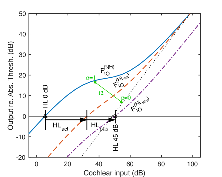
A.1 Cochlear IO function and formulation of HL
Figure 6 shows a schematic diagram of the cochlear IO function. The cochlea contains OHCs that amplify the basilar membrane vibrations in response to faint sounds. For an NH person, the IO function ( represented by the blue line) does not increase linearly with increasing input levels; rather, it increases gradually. This is referred to as a compressive characteristic. If there is a dysfunction in the active amplification, the IO function becomes (red broken line). The compression health parameter (green) was introduced to represent this difference. When , coincides with , i.e., the NH curve with no dysfunction. When , coincides with the black dotted line representing linear growth. This indicates that active amplification is completely damaged.
Furthermore, when IHCs, which convert vibration to neural firing, are dysfunctional, the output decreases, resulting in (purple dotted line). When viewed in terms of the absolute threshold corresponding to the audiogram (on the horizontal line where output is 0 dB), the total hearing loss can be expressed as the sum of the active loss and the passive loss in dB [Irino, 2023]. This formulation is also used in a loudness model by Moore et al. [1997].
| (8) |
A.2 Apportionment of HL
Although the above formulation is sufficiently simple, it is not possible to determine the ratio of to or from an individual audiogram alone. To determine this, an accurate estimation of the slope of is necessary. Ideally, the estimation experiments would take as little time as audiometry tests. However, this is challenging as described in the next subsection. Therefore, this study uses the preset value of , as did previous studies.
Even if the preset is , the lower limit of is automatically determined so that it does not fall below the hearing level (). Therefore, the practical value of different among audiometric frequencies and individual listeners (e.g., Irino et al., 2024). The proportion of has been reported to be relatively high at low frequencies [Schlittenlacher & Moore, 2020]. Therefore, we consider setting to be generally adequate, although the exact details remain unclear.
A.3 Estimation of the IO slope and its limits
Three methods for estimating the IO slope have been considered thus far.
-
1.
Estimating the IO function using the notch noise simultaneous masking method and a level-dependent auditory filter, such as a compressive gammachirp [Patterson et al., 2003, Irino et al., 2023]. This method does not involve difficult experimental tasks. However, it requires a large number of measurement points, making it much more time-consuming than an audiometry test.
-
2.
Loudness matching by patients with unilateral HL [Moore & Glasberg, 1997]. Since loudness functions and cochlear IO functions are thought to be closely related, this is a reasonable direct measurement method. However, unilateral HL and age-related HL may have different underlying mechanisms. Additionally, age-related HL generally progresses simultaneously in both ears, making this method inapplicable.
-
3.
A method for directly determining the IO function using the time masking curve (TMC) method Nelson et al. [2001]. This is a forward masking paradigm with a very short detection signal. Estimation results for individuals with moderate HL have also been reported Lopez-Poveda et al. [2005]. We implemented this method as well, but the short signals were difficult to detect, even with auxiliary sounds. Considerable training is required for even NH individuals to perform the task, and the method is not simple.
Each method has its own set of challenging drawbacks. However, the IO slope cannot be estimated without conducting such experiments that are much more extensive than SI experiments. A new method is necessary to measure the slope in a time comparable to that of audiometry tests.
Because these experiments were not conducted as part of this study, it was impossible to estimate the slope or value for each older adult. However, it could be assumed that older adults may have some degree of active HL. Therefore, it is more reasonable to assume that an value of 0.5 than to assume they have values of 1 (completely healthy) or 0 (completely damaged).
Note that any recent level-dependent, nonlinear auditory filterbank should consider the slope of the IO function (or equivalently, ) to reliably simulate the cochlea. It is unreasonable to assume that the slope is automatically determined from the hearing level, as HASPIv2 and HASPIw2 do, because these are independent parameters, as described in A.2.
Appendix B Measurement of TMTF
For estimating the temporal processing characteristics of participants, the TMTF measurements [Viemeister, 1979] were conducted using the two-point method proposed by Morimoto et al. [2019]. This method approximates the TMTF as a first-order low-pass filter (LPF) and attempts to determine its parameters using only two measurement points, allowing rapid measurement as in audiometry.
The carrier of the stimulus sound is low noise [Pumplin, 1985, Kohlrausch et al., 1997], which is a broadband noise with minimized envelope fluctuation. The envelope is modulated by a sine wave as
| (9) | |||||
| (10) |
where is a modulation depth, is a modulation frequency, and is time. is a factor to keep the SPL constant over .
First, the detection threshold of the unmodulated noise was measured for each participant. Using this value, the signal level was set to 20 dB SL so that the signal was presented well above the threshold. Thus, the SPL was individually different. Then, the detection threshold to determine the TMTF was measured by the transformed up-down method with 3-interval, 3-alternative forced-choice and 1 up - 2 down procedure [Levitt, 1971]. The modulation depth threshold, in dB, was measured in the noise modulated at a frequency of 8 Hz. This value was taken as the peak sensitivity at low modulation frequencies () in dB. Next, the modulation depth was set to in dB and the modulation frequency was varied to measure the threshold (Hz), which is the upper limit of the detectable frequency.
From these values, the cutoff frequency of the LPF () can be calculated using the following formula:
| (11) |
At this point, the TMTF in dB is given by the following equation:
| (12) |
Figure 2 shows the TMTF for left and right ears of individual listeners. Note that the average values for the NH listener were estimated as -23 dB and 128 Hz in Morimoto et al. [2019].
Appendix C Speech enhancement using IRM
Noisy sounds can be formulated as
| (13) |
where is a sample time; , , , and are the speech sound at the listener's ear, the original clean speech, the impulse response of the acoustic environment, and the noise. The purpose of SE is to reduce the noise from the observed signal .
A time-frequency representation of this can be derived by applying the short-time Fourier transform.
| (14) |
where and are the time and frequency frame indexes, respectively. The Ideal Ratio Mask (IRM) [Wang et al., 2014] is formulated as:
| (15) |
where the powers of the signal and noise are known in advance to provide the ideal SE performance. Using this mask , the enhanced time-frequency representation can be derived as
| (16) |
The enhanced sounds are derived by overlapping and adding the inverse short-time Fourier transform of . In this study, the process was performed at a sampling frequency of 16 kHz with a frame duration of 64 ms (hanning window) and a frame shift of 16 ms. The sound clarity was better when 16 kHz was used than when 48 kHz was used, probably due to the effect of high frequency components.
Appendix D Evaluation of GESI with CPC2 data
In the main text, GESI and HASPIw2 were evaluated using familiarity-controlled Japanese words. We found that HASPIw2 does not generalize well to Japanese data. However, it remains unclear whether GESI can generalize sufficiently to English.
D.1 Speech data for evaluation
The ideal approach to addressing this issue would be to conduct a listening experiment with English words that are controlled for familiarity, similar to the experiment conducted in this study. Although Posoni's group provided a database of familiarity ratings in Nusbaum et al. [1984], no speech data were available and no speech-in-noise experiments were performed. More recently, Braza et al. [2022] conducted a speech-in-noise experiment with familiarity-controlled words. However, their study did not include an evaluation by older adults or the validity of the OIM. Additionally, the speech data used in their experiments is not publicly available. Given these limitations, conducting a thorough validation study using familiarity-controlled English words would require the development of a new dataset, which is beyond the scope of this study.
Therefore, we chose to use the publicly available CPC2 dataset [Barker et al., 2024] as an alternative. This dataset includes large-scale speech and the corresponding sentence-level (SI) scores of English sentences (see D.3). However, sentence-level prediction is inherently challenging for bottom-up models like GESI because they do not incorporate linguistic information. We addressed part of this issue with strategies that will be described in D.2.1.
D.2 Method
We compared HASPIv2 and GESI using the CPC2 dataset. HASPIv2 contains NNs that were trained using English sentences. It was employed as a baseline model in the CPC2 competition, where performance was evaluated using sentence SI. Although HASPIw2 was used for comparison with GESI in the main text, it is not suitable for predicting sentence SI. Furthermore, there was also a practical issue. CPC2 provides an evaluation environment using Python. It included a Python version of HASPIv2, but not HASPIw2. Thus, HASPIw2 could not be evaluated. In order to enable a comparison in this environment, we created a Python version of GESI based on the original MATLAB version.
Because of its contextual modeling through NNs, HASPIv2 is expected to be much more advantageous than GESI. Nevertheless, we would like to know how well GESI performs with English sentences. GESI was originally developed to predict SI for short segments, such as words. Therefore, additional processing was necessary to estimate sentence-level SI. In this study, we employed a simple strategy. First, we segmented each sentence into individual words. Then, we computed GESI scores for each word and combined them to predict the overall sentence SI as described in D.2.4. The following sections provide more detail on the procedures used for GESI and describe the data used in the evaluation.
D.2.1 Word-wise computation and binaural processing
First, we applied the Whisper automatic speech recognizer [Radford et al., 2023] to the reference signal in order to obtain word-level timestamps. Then, we used this information to divide the reference and test signals into word-level segments. The word-level signal pairs were used as input for GESI. To capture all acoustic features and prevent truncation and clipping at the boundaries, the word duration was extended by 50 ms at the beginning and end.
SI scores were calculated independently for the signals from the left and right ears. The higher of the two scores for each word was chosen as the final value. This better-ear approach is also used to compute HASPIv2 scores in the CPC2.
D.2.2 Parameter setting
Hearing levels were used in the calculation independently for the left and right ears. Missing data was supplemented by extrapolating or interpolating from existing values. As in the main text and A, a fixed value of was used for the compression health parameter, , for all listeners. The most confusing aspect of the CPC2 dataset is the lack of information about SPLs at specific digital levels. The metadata of each audio file contained a ``volume'' field ranging from 0 to 100, with a default of 50. However, there is no information about the correspondence between volume and SPL. Therefore, we could not perform SI calculations as precisely as those described in the main text. But for the best guess, we assumed that an RMS value of 1 corresponds to a playback level of 120 dB SPL.
D.2.3 Ground truth data
We evaluated the accuracy of the predictions for the subjective response data in the CPC2 challenge. The CPC2 response data included the following: (1) the text of the speech presented to listeners (prompt); (2) the transcribed text of listeners' responses; (3) the number of words in the prompt (nwords); (4) the number of correctly identified words (hits); (5) the percentage of correctly identified words (correctness = hits/nwords*100), ranging from 0 to 100%. This correctness is the definition of sentence SI in CPC2 and is used as the ground truth.
D.2.4 Prediction method
As mentioned earlier, GESI was not designed to predict sentence SI. Therefore, we adapted the following simple strategy: First, we calculated the GESI score of each word in the sentence. Then, we set a threshold value, which will be described below. If a word's score is above the threshold, we assume that the word has been correctly identified and count it as a hit. Finally, we calculated the correctness as described above, and treated it as the predicted sentence SI.
This strategy requires determining an adequate threshold. We compiled a list of all the words in the evaluation dataset. For each word, there is a GESI score and a listener's binary ``hit-or-miss'' label. Then, we calculated the ROC curve using the true positive rate (TPR) and the false positive rate (FPR) at various GESI score thresholds. The optimal threshold was determined to be the one that maximizes the Youden index, [Youden, 1950], which is equal to the TPR minus the FPR. Note that this strategy does not provide any contextual information within the sentences. Therefore, the GESI prediction did not use that information.
D.3 Dataset
First, we briefly describe the original CPC2 dataset [Akeroyd et al., 2023, Barker et al., 2024] to provide an overview of the speech sounds presented to listeners. Then, we explain how the subset was selected for this study.
D.3.1 Original CPC2 dataset
The CPC2 dataset includes speech-in-noise data processed by hearing aids, as well as the listening responses for people with a HL. These signals were generated for the 2nd Clarity Enhancement Challenge (CEC2) [Akeroyd et al., 2023]. The target speech materials were the Clarity Speech Corpus: seven- to ten-word sentences recorded by British English speakers [Graetzer et al., 2022]. These sentences were selected from the British National Corpus XML edition [BNC Consortium, 2007]. The sentences were filtered to exclude those containing one or more unusual words. An unusual word is defined as a word not found in the database of Kučera & Francis [1967]. Multiple noise sources, such as music, speech, or domestic appliance noises, were added to these clean utterances at SNRs between -12 dB and +6 dB. The clean utterances were added multiple noise sources, such as music and speech. The speech-in-noise signals were convolved with head and room impulse responses (HRIRs) to reproduce complex and realistic listening scenarios.
The speech sounds have been processed using ten hearing aid algorithms submitted to CEC2 [Akeroyd et al., 2023]. The algorithms varied depending on whether the approach was single-channel enhancement, multichannel processing, or signal amplification. For the listening tests, personalized stereo signals were produced using pairs of hearing aid input signals and the left and right audiograms of the participants, with HL. Participants took the listening tests in their own homes. They used headphones and a tablet PC, and did not wear their hearing aids. The listeners controlled the volume on the tablet. This is why the SPL could not be precisely controlled.
The CPC2 dataset included training and evaluation data. The training data contained listener responses and signal information from the listening tests. However, this information was not included in the evaluation data.
D.3.2 Selected dataset for this evaluation
We only use training sets because listener responses are available. There were three separate training sets, which included responses by fifteen listeners in total. We randomly selected ten sentences from each listener, resulting in a subset of 150 sentences. Therefore, the subset contains roughly 1000 words. This subset was used to compare the sentence-level SI prediction performance of GESI against HASPIv2.
The fifteen listeners were split into two groups. Five listeners were used to determine and in the sigmoid function in Eq. 3 (i.e., closed evaluation), and the remaining ten listeners were used for open evaluation.
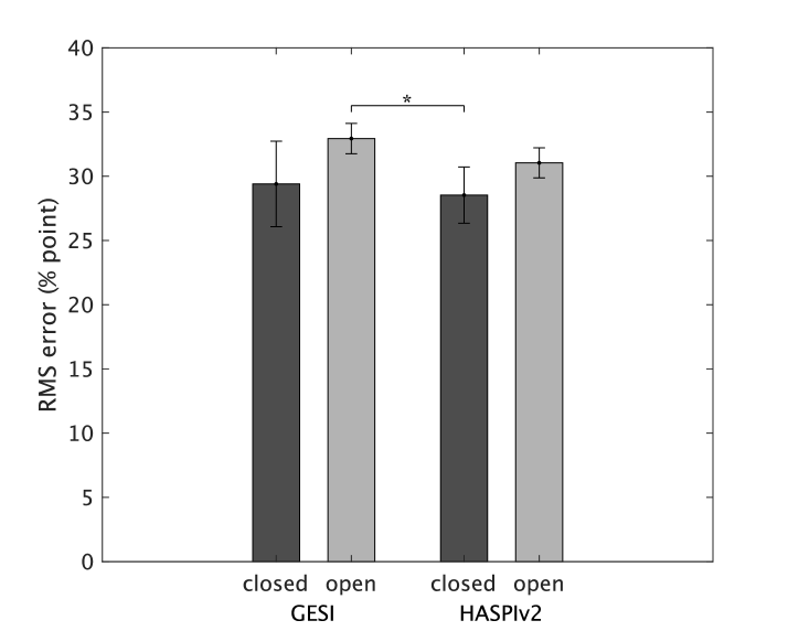
D.4 Prediction performance of sentence SI
To ensure a robust evaluation across different data splits, we repeated the random split procedure ten times, as described in Section 4.4. For each split, we predicted sentence-level SI scores using both GESI and HASPIv2. We evaluated the prediction performance using the RMS error obtained under each data condition.
For each split, RMS errors were calculated for each listener. Then, the results were averaged. The averaged RMS errors across the ten splits were then used for statistical analysis. Figure 7 shows the results. In the closed dataset, the mean RMS error for GESI is 0.87 % points higher than that for HASPIv2; and in the open dataset, it is 1.9 % points higher. Since HASPIv2 is trained to predict the sentence-level SI, this result is considered reasonable. We also conducted a three-way ANOVA to examine the effects of the evaluation condition (closed versus open), the OIM (GESI versus HASPIv2), and repetition of the prediction. The main effects of the OIM and repetition were not significant. However, the main effect of the evaluation condition was significant (). None of the interactions were significant. Tukey's HSD tests revealed no significant differences between the conditions, except for one pair, which is shown in Fig. 7. This suggests that GESI is at least as effective as, if not more effective than, HASPIv2. Considering that GESI did not use contextual information, its performance seems satisfactory.