2 State Key Laboratory of Information Engineering in Surveying, Mapping and Remote Sensing, Wuhan University, Wuhan 430079, China
3 School of Resource and Environment, Hubei University of Science and Technology, Xianning, Hubei, China
∗ Corresponding author: wbshen@sgg.whu.edu.cn
Preliminary experimental results of determining the geopotential difference between two synchronized portable hydrogen clocks at different locations
Abstract
According to general relativity theory (GRT), by comparing time elapses between two precise clocks located at two different stations, the gravity potential (geopotential) difference between them can be determined, due to the fact that precise clocks at positions with different geopotentials run at different rates. Here, we provide preliminary experimental results of the geopotential determination based on time elapse comparisons between two remote atomic clocks located at Beijing and Wuhan, respectively. After synchronizing two hydrogen atomic clocks at Beijing 203 Institute Laboratory (BIL) for 20 days as zero-baseline calibration, namely synchronization, we transport one clock to Luojiashan Time-Frequency Station (LTS), Wuhan, without stopping its running. Continuous comparisons between the two remote clocks were conducted for 65 days based on the Common View Satellite Time Transfer (CVSTT) technique. The ensemble empirical mode decomposition (EEMD) technique is applied to removing the uninteresting periodic signals contaminated in the original CVSTT observations to obtain the residual clocks-offsets series, from which the time elapse between the two remote clocks was determined. Based on the accumulated time elapse between these two clocks the geopotential difference between these two stations was determined. Given the orthometric height (OH) of BIL, the OH of the LTS was determined based on the determined geopotential difference. Comparisons show that the OH of the LTS determined by time elapse comparisons deviates from that determined by Earth gravity model EGM2008 by about 98 m. The results are consistent with the frequency stabilities of the hydrogen atomic clocks (at the level of /day) applied in our experiments. Here the EEMD technique was first introduced and applied in the subjects related to this study, especially for the purpose of removing the periodic signals from the original CVSTT observations to obtain the residual clock offsets signals, from which one can more effectively extract the geopotential-related signals. In addition, we used 85-days original observations to determine the geopotential difference between two remote stations based on the CVSTT technique. Using more precise atomic or optical clocks, the CVSTT method for geopotential determination could be applied effectively and extensively in geodesy in the future.
keywords:
relativistic geodesy, atomic clock, CVSTT technique, EEMD technique1 Introduction
Precise determination of the Earth’s geopotential field and orthometric height (OH) is a main task in geodesy (Mazurova et al.,, 2012, 2017). With rapid development of time and frequency science, high-precision atomic clock manufacturing technology (Hinkley et al.,, 2013; Bloom et al.,, 2014; McGrew et al.,, 2018) provides an alternative way to precisely determine the geopotentials and OHs, which has been extensively discussed in recent years (Bondarescu et al.,, 2012; Shen et al.,, 2016; Lion et al.,, 2017; Shen et al.,, 2018), and opening a new era of time-frequency geoscience (Kopeikin et al.,, 2018; Shen et al.,, 2019).
General relativity theory (GRT) states that a precise clock runs at different rates at different positions with different geopotentials (Einstein,, 1915). Based on GRT, Bjerhammar, (1985) proposed an idea to determine the geopotentials via clock transportation. Later, Shen et al., (1993) put forward an approach to determine geopotentials via gravity frequency shift (GFS) that is also based on GRT. Consequently, the geopotential difference between two arbitrary points can be determined by comparing the running rates of two precise atomic clocks (Bjerhammar,, 1985; Mai and Müller,, 2013) or by comparing their frequencies (Shen et al.,, 1993; Shen,, 1998; Shen et al., 2009b, ; Shen et al.,, 2011). In order to determine geopotentials with an accuracy of 0.1 m2s-2 (equivalent to 1 cm in OH), the atomic clocks with frequency stabilities of are required.
High performance clocks and time-frequency transfer techniques have been intensively developing over the past 60 years (Akatsuka et al.,, 2008; Bondarescu et al.,, 2015; Mehlstäubler et al.,, 2018). Recently, optical-atomic clocks (OACs) with stabilities around level have been successively generated (Nicholson et al.,, 2015; Campbell et al.,, 2017; McGrew et al.,, 2018), and in the near future mobile high-precision satellite-borne optical clocks will be in practical usage (Poli et al.,, 2014; Singh et al.,, 2015; Riehle,, 2017). This provides a good opportunity to precisely determine the geopotentials via precise clocks. Therefore, high-precision clocks enable 1 cm level geopotential determination and the realization of world height system (WHS) unification (Shen et al.,, 2016; Koller et al.,, 2016; Müller et al.,, 2018).
As mentioned before, there are two kinds of methods for determining the geopotentials via clocks. One method is to compare the time elapses of two clocks located at two stations using various techniques (Bjerhammar,, 1985; Shen and Shen,, 2015; Kopeikin et al.,, 2016). The other method is to compare frequency difference of the two clocks (Shen et al.,, 2017, 2018; Deschenes et al.,, 2015; Pavlis and Weiss,, 2017). It is true that there exist some successful transportation experiments for determining geopotential via high-precise fiber links (Lisdat et al.,, 2016; Takano et al.,, 2016; McGrew et al.,, 2018; Grotti et al.,, 2018), and the corresponding results are quite successful. For example, Grotti et al., (2018) provided the transportation experiments by using optical atomic clocks for their unprecedented stability, and the discrepancy between relativistic method and conventional method variates 2 42 in geopotential units. However, there are seldom transportation experiments using the satellite signals for comparing clock offsets in the relativistic geodesy. In fact, satellite time and frequency signal transfer approach is most prospective in the future due to the fact that it is not constrained by geographic conditions, for instance connecting two continents separated by oceans. Kopeikin et al., (2016) discussed and provided experimental results of transportation experiments for geopotential difference determination via Common-View Satellite Time Transfer (CVSTT) technique, with the help of two hydrogen atomic clocks. The results are consistent with the clocks’ stabilities in their experiments with a discrepancy of hundreds of meters. However, in their experiments, the time comparison period is quite short. For instance, the geopotential difference measurement lasted about 63900 s (17.7 hr), and the zero-baseline calibration lasted only 23790 s (6.6 hr).
In this study, we focus on the clocks’ time elapse comparisons via the CVSTT technique, and the determination of geopotential difference based on clock transportation experiments. Here, the transportation experiments last for a quite long time, with the zero-baseline measurement lasting for 20 days, and the geopotential difference measurement lasting for 65 days with plenty of data sets. In addition, we first use the EEMD technique to remove the uninterested periodic signals from the original CVSTT observations to obtain the residual clock offsets signals, and then extract the geopotential-related signals from the residual clock offsets signals. In our knowledge, this is a first application in CVSTT data processing for the purpose of determining the geopotential difference in geodetic community. In this study, the stability of H-masers used in the experiments is at /day level, which means that the determination of geopotential difference is limited to tens of meters in equivalent height. We admit that the performance of the H-masers cannot be compared to the optical atomic clocks with unprecedented stability, and it cannot obtain perfect results like the optical atomic clocks via optical fiber. However, the H-masers have their special advantages, for example, they can keep operation with a relative stable stability for a long period, which could be difficult for the optical atomic clocks at the current stage. In the future, the optical atomic clock might be introduced in the similar experiments when the experimental conditions are mature.
This paper is organized as follows. In Section 2, we briefly describe how to determine geopotential as well as OH using two remote clocks. In Section 3, we focus on describing how to achieve the comparisons of time elapses between two remote clocks based on the CVSTT technique, and how to cancel or greatly reduce various error sources. In Section 4, we introduce ensemble empirical mode decomposition (EEMD) technique, and verify its effectiveness for extracting the linear signals of interest from the original CVSTT observations based on simulation experiments. In Section 5, we describe our experimental setup, records, and data procession. We provide experimental results and relevant discussions in Section 6, and draw conclusions in Section 7.
2 Method
Based on GRT, considering the proper time durations and recorded by two precise clocks and located at two stations and , respectively (see Fig. 1). Accurate to , the following equation holds (Weinberg,, 1972; Bjerhammar,, 1985; Shen et al., 2009a, ; Mehlstäubler et al.,, 2018):
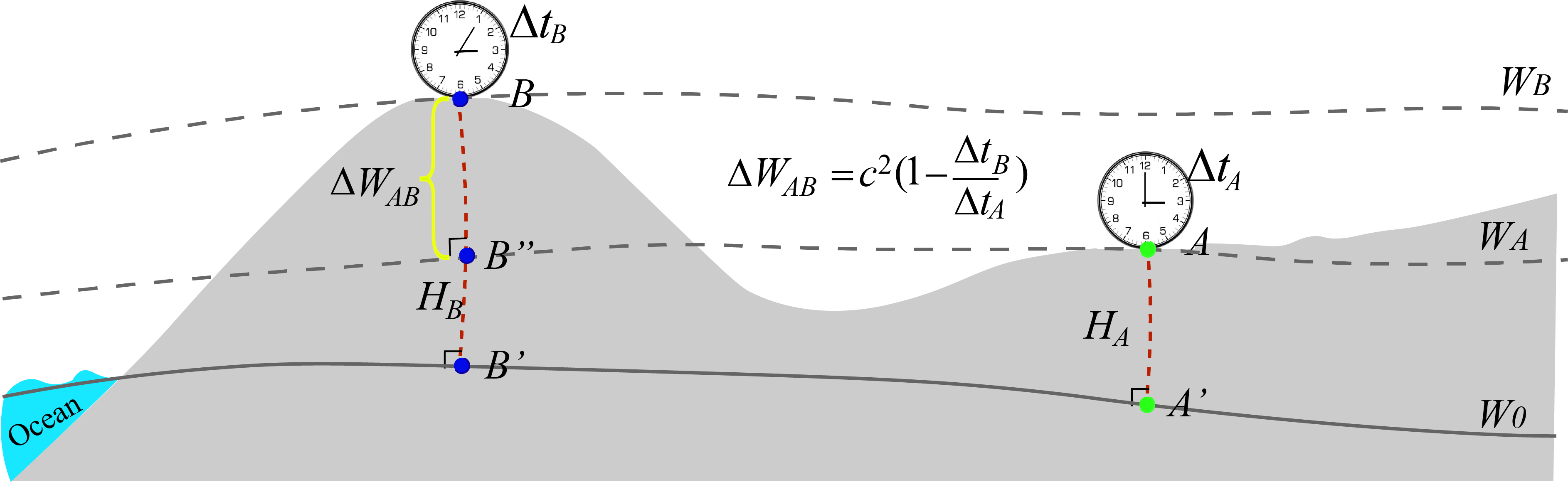
| (1) |
where denotes a standardized time duration (measured by a standard clock at infinity or at the center of the Earth); denotes the elapsed time of clock (); denotes geopotential at station ; m/s is the speed of light in vacuum.
Here, we point out that, the deformation of the Earth surface caused by the tides are neglected, due to the fact that the tidal influences are at tens of centimeters level. Considering the stability of the hydrogen atomic clocks used in the experiments, say at /day level, which is equivalent to tens of meters in OH, the effect caused by the tidal influences is much smaller (two orders of magnitude lower). In the future study, however, when the clock’s stability reaches level, the tidal effects should be considered carefully.
From formula (1), the clock-comparison-determined geopotential difference between stations A and B, can be expressed as follows (accurate to ):
| (2) |
The OH can be determined based on the following expression (Molodenskii,, 1962; Heiskanen and Moritz,, 1967; Jekeli,, 2000):
| (3) |
where is the geopotential on the geoid, with 62636853.4 0.02 m2s-2 (Sánchez et al.,, 2016; Sánchez and Sideris,, 2017), is the geopotential at location , is the ’mean gravity value’ at a particular point on the segment of the plumb line between point and .
Suppose the geopotential at station A is a priori given, by combining formulas (2) and (3), the clock-comparison-determined OH at staion B, can be determined as follows:
| (4) |
Finally, by combining formulas (3) (4) we can compare the discrepancy between clock-comparison-determined results () with the corresponding results determined by conventional approach ():
| (5) |
where can be determined by levelling and gravimetry or directly determined by a given Earth gravity model. In this study we use EGM2008 to obtain the geopotentials and .
The determination of as well as requires a precise measurement of time comparison. Hence, one practical solution is to set clock as the standard, after a standard time elapses , the clock elapses , correspondingly. Therefore, the time elapse difference between clocks and , can be finally determined as follows (Shen and Shen,, 2015):
| (6) |
To realize a precise time comparison between two remote clocks, we need not only atomic clocks with high stability for maintaining the standard time elapse, but also a reliable time transfer technique that can precisely measure the time elapses.
3 Common-View Satellite Time Transfer Technique
3.1 CVSTT technique
As early as in 1980, it was proposed that the CVSTT technique could be used for comparing clock offsets between two remote clocks (Allan and Weiss,, 1980; Allan et al.,, 1985). This technique was adopted by the Bureau International des Poids et Mesures (BIPM) as one of the main methods for transferring international atomic time (TAI) signals (Allan and Thomas,, 1994; Imae et al.,, 2004). Using this method, the uncertainty of comparing remote time may achieve several nanoseconds (Lewandowski and Thomas,, 1991; Lewandowski et al.,, 1999; Ray and Senior,, 2003; Sun et al.,, 2010; Yang et al.,, 2012; Rose et al.,, 2016). The main advantages of CVSTT technique lie in that the satellite clock errors are cancelled, and various other errors, especially ionospheric and tropospheric errors, are largely reduced due to the simultaneous two-way observations (Allan and Weiss,, 1980; Yang et al.,, 2012; Defraigne and Baire,, 2011).
In this study, we use the CVSTT technique for comparing the clock offsets. The reasons are stated as follows. Firstly, the CVSTT technique is a stable and accurate method for comparing clock offsets between two remote clocks, and this technique has been adopted by the Bureau International des Poids et Mesures (BIPM) as one of the main methods for transferring international atomic time (TAI) signals. Therefore, the results of CVSTT technique are reliable and stable. Secondly, using CVSTT technique is relative cheap and convenient in practice. Though the experimental results using optical atomic clocks via fiber links are quite accurate and stable indeed, the fiber-link is limited to a relative short distance and fixed stations with fiber links, and for a long distance even intercontinental comparison, the fiber-link is extremely challengeable and costly. In addition, the Two-way satellite time and frequency transfer (TWSTFT) technique is more accurate and stable than CWSTFT technique, but it is very expensive in economy, which could be applied in the future when the condition is available. Lastly, though the carrier phase measurements in GNSS are more precise than the corresponding precise code measurements in time transfer, the absolute clock offsets cannot be determined from carrier phase measurements due to the ambiguities issues (Defraigne and Bruyninx,, 2007). Therefore, the code measurements are necessary for determining the absolute clock offsets between remote time and frequency standards for a long time. Hence, at present experiment condition, the CVSTT technique and precise code measurements are adopted here.
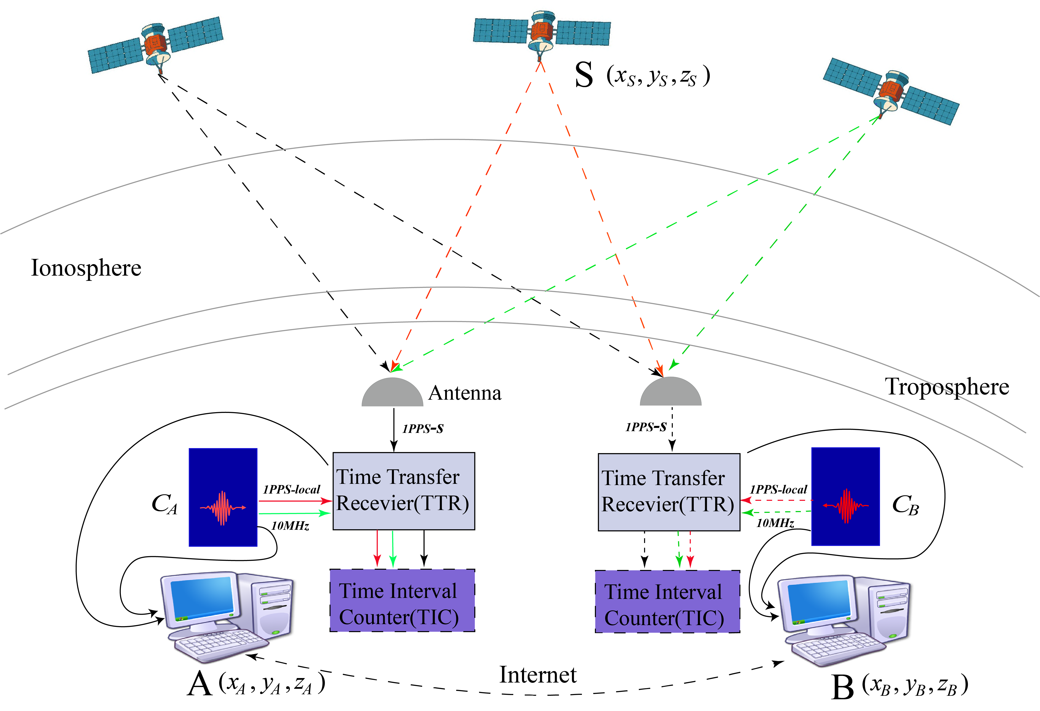
To better understand the text, here we briefly introduce the principle of the CVSTT technique. Suppose there are two ground stations (, ) and a common-view satellite . The coordinates of the two ground stations are denoted as (), and the satellite coordinates are denoted as (). At an appointed time, the -th staion’s clock and satellite’s clock emits 1 purse per second (1 PPS) signals, simultaneously. The 1 PPS signal of the -th station (denoted as 1PPS-local signal) arrives to the GNSS time transfer receiver (GNSS-TTR) via cables, and opens the door of the time interval counter (TIC) for starting timing. At the same time, the 1PPS signal of the satellite (denoted as 1PPS-S signal) is received by the GNSS antenna of the ground station. After signals demodulation the 1PPS-S signal arrives to the GNSS-TTR via cables. And the 1PPS-S signal is used for closing the TIC’s door for stopping timing. The -th staion’s clock also generates the 10 MHz sinusoidal signals with extremely high accuracy. Therefore, for the -th station and at a certain timepoint, by counting the number of the sinusoidal waves between the starting timepoint (the time of 1PPS-local signals arrive at TIC) and the stopping timepoint (the time of 1PPS-S signals arrive at TIC), the time interval between the two 1PPS signals can be determined as follows (Allan and Weiss,, 1980; Lee et al.,, 1990; Lewandowski and Thomas,, 1991):
| (7) |
where is time interval measurement of the two 1 PPS signals at station ; and are the emission timepoints of 1PPS signals of the atomic clocks from -th station and satellite , respectively; is the error source (e.g. ionospheric delay, tropospheric delay, and Sagnac effect); is the receiver delay which is usually calibrated by the manufacturing company using simulated signals (Lewandowski and Thomas,, 1991); and is the geometric distance between -th station and satellite , expressed as:
| (8) |
By applying equation (7), the clock offsets between the -th station and satellite S can be expressed as follows:
| (9) |
Finally, the clock offsets between two ground stations A and B can be determined by taking the common-view satellite’s clock as common reference:
| (10) |
We note that the cable delays from station’s atomic clock to TTR are measured beforehand with the value of 50.2 ns, as well as the cable delays from GNSS antenna to TTR with the value of 204.5 ns. And the cable delays are input into the TTR as a parameter. In fact, the cable delays are not significant in our study due to the fact that we compare the time elapse between two remote clocks.
3.2 Error sources
3.2.1 Satellite position Error
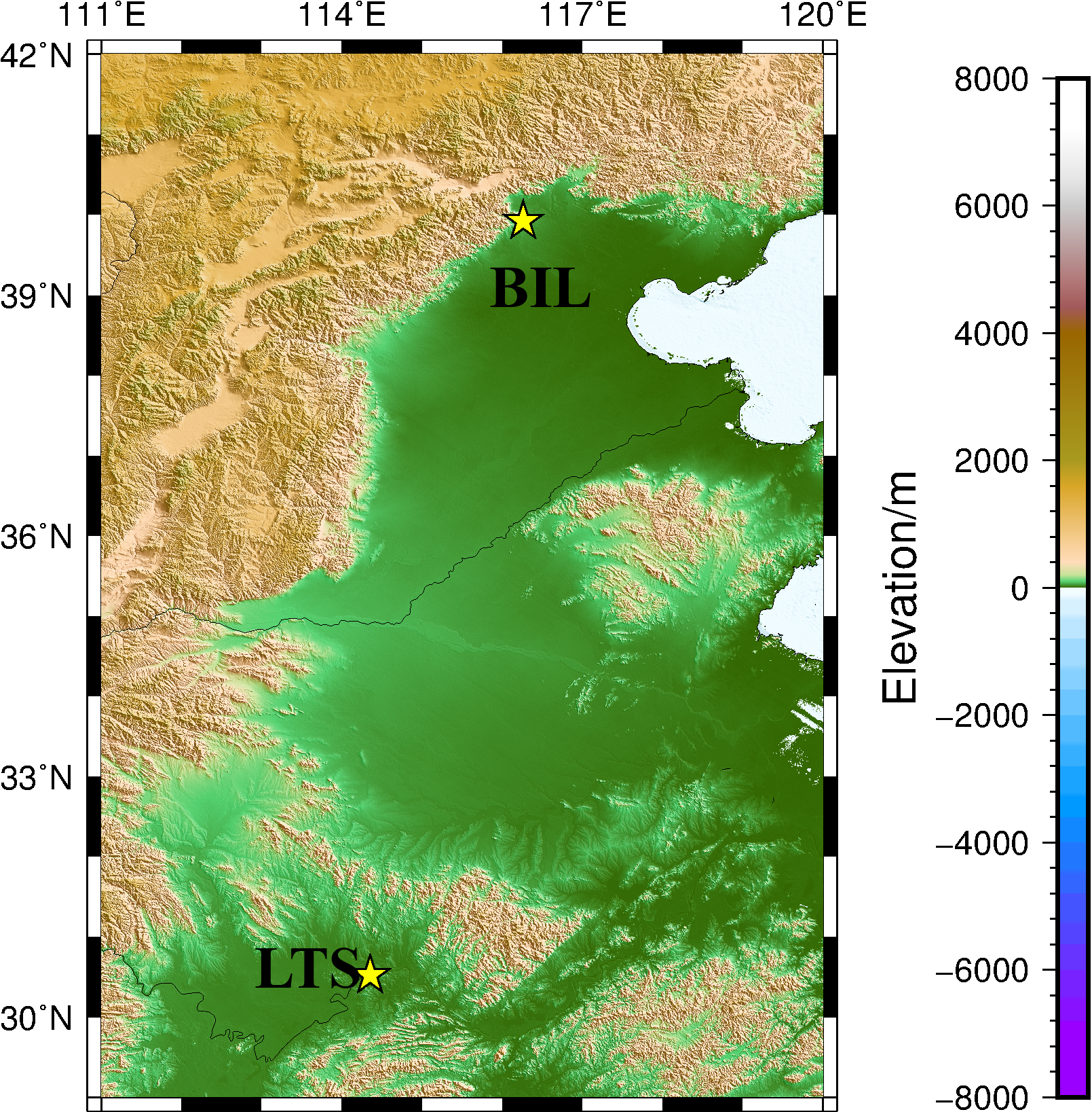
In this study, the transportation experiments is conducted at Beijing 203 Institute Laboratory (BIL) and Luojiashan Time-Frequency Station (LTS). In the sequel, we analyze various error sources.
The accuracy of the satellite positions depends on the ephemeris. The broadcast ephemeris is adopted in conventional CVSTT technique. Suppose the satellite position error is (, , ), when ignoring the position error of ground stations, the relation between satellite position error and time transfer error in CVSTT technique can be determined by using the first-order difference (Imae et al.,, 2004; Li et al.,, 2008; Sun et al.,, 2010):
| (11) |
where
| (12) |
Based on formulas (11) and (12) and applying the error propagation law, the following expression can be obtained:
| (13) |
For instance, when accuracy of broadcast ephemeris in individual axes is 2 m (Gao,, 2004; Liu et al.,, 2017), the accuracy of time transfer error caused by satellite position error did not exceed 0.16 ns in the experiments. The influences of the ground stations’ positions errors on the time transfer in CVSTT technique can be evaluated, similarly. Here the ground stations’ coordinates are determined based on the precise point positioning (PPP) method in advance, with accuracy level of better than 3 cm (Dawidowicz and Krzan,, 2014), and the corresponding time transfer error caused by the coordinates errors will not exceed 0.15 ns (see Table 1).
3.2.2 Ionospheric effect
The ionospheric effect on GNSS signal means a signal delay which could achieve several tens of nanoseconds, due to the electron content of the atmospheric layer. And the effect becomes more dramatic during an ionospheric storm. The zenith group delays are about 1 30 m, 02 cm, and 02 mm for the first-, second- and third-order ionospheric effects, respectively (Bassiri and Hajj,, 1993; Marques et al.,, 2011; Zhang et al.,, 2013). For the GNSS time transfer receivers, measurements on two frequencies ( and ) are often available. Therefore, an ionosphere-free observation can be constructed so that the first-order term of ionospheric effect can be removed completely, due to the fact that the ionospheric effect on a signal depends on its frequency. The is constructed as follows (Petit and Arias,, 2009; Peng and Liao,, 2009):
| (14) |
where and are the precise-code observations with frequencies of MHz and MHz, respectively.
However, formula (14) only removing the first-order ionospheric effect. There are second- and third-order ionospheric effects (also denoted as higher-order ionospheric effects). The residual higher-order ionospheric effects, , can be expressed as follows (Morton et al.,, 2009):
| (15) |
where is the number of electrons in a unit volume(), is the magnitude of the plasma magnetic field(T), is the angle between the wave propagation direction and the local magnetic field direction, and is the integral path. More details can be seen in Morton et al., (2009) and Zhang et al., (2013).
By using CVSTT technique, the residual errors of ionospheric effects between ground stations A and B, , can be determined as follows:
| (16) |
By using the constructed ionosphere-free observation , we remove the first-order ionospheric effect, which contributes to more than 99% of the entire ionospheric effects (Defraigne and Baire,, 2010; Harmegnies et al.,, 2013; Huang and Defraigne,, 2016), and the residual errors of higher-order terms are about 24 cm (Bassiri and Hajj,, 1993; Morton et al.,, 2009; Deng et al.,, 2015).
On the other hand, the code noise should be taken into consideration carefully. Suppose code noise of and are and , respectively. By applying the error propagation law, the code noise of ionosphere-free observation, , can be expressed as follows:
| (17) |
Here, suppose the code noise , and take the values of MHz and MHz into formula (17), the relations of can be obtained. The accuracy of P code measurement is about 0.29m, which is equivalent to 0.97 ns in time. Therefore, the accuracy 2.89 ns of the code measurement is determined, and the corresponding time transfer accuracy of the time interval measurement in CVSTT technique, , will not exceed 4.09 ns. Combining expressions (16) and (17), after implementation of strategy of ionosphere-free combination, the residual ionospheric errors in CVSTT technique will not exceed 0.8 ns (see Table 1).
3.2.3 Tropospheric effect
The troposphere is the lower layer of atmosphere that extends from ground to base of the ionosphere. The signal transmission delay caused by troposphere is about 220 m from zenith to horizontal direction (Xu,, 2007; Chen et al.,, 2012). The tropospheric delay depends on temperature, pressure, humidity, and as well as location of the GPS antenna (Feng et al.,, 2006). The total tropospheric delay can be divided into hydrostatic part and wet part, which can be expressed as follows (Boehm and Schuh,, 2004; Kouba,, 2008):
| (18) |
where is the total tropospheric delay, and are the hydrostatic part and wet part in zenith delays, respectively. and are the corresponding mapping functions (MF), respectively. MF is a function of , , , and , E is the elevation angle in radian. , , and are MF coefficients.
Boehm and Schuh, (2004) introduced a rigorous approach for utilizing the Numerical Weather Models (MWM) for MF determinations. The first and most significant MF coefficients, and , are fitted with the NWM from the European Centre for Medium-Range Weather Forecasts (ECMWF). The coefficient , and coefficient is expressed as follows:
| (19) |
where is the day of the year; is the latitude; , , and specifies the Northern or Southern Hemisphere, respectively. For the wet part, the coefficients and are constants with and (Boehm et al.,, 2006).
Then, the gridded VMF1 data is generated from the ECMWF NWM using four global grid files() of , , and . Using VMF1, one can determine the tropospheric delay at any location after 1994 (Kouba,, 2008). The tar-compressed files of all VMF1 epoch grid files are available at the VMF1 website (http://ggosatm.hg.tuwien.ac.at/DELAY/GRID/VMFG/). More details are available in Boehm and Schuh, (2004) and Kouba, (2008).
To achieve near real-time data processing and improve efficiency, a simple empirical model is employed, which is expressed as follows (Parkingson et al.,, 1996):
| (20) |
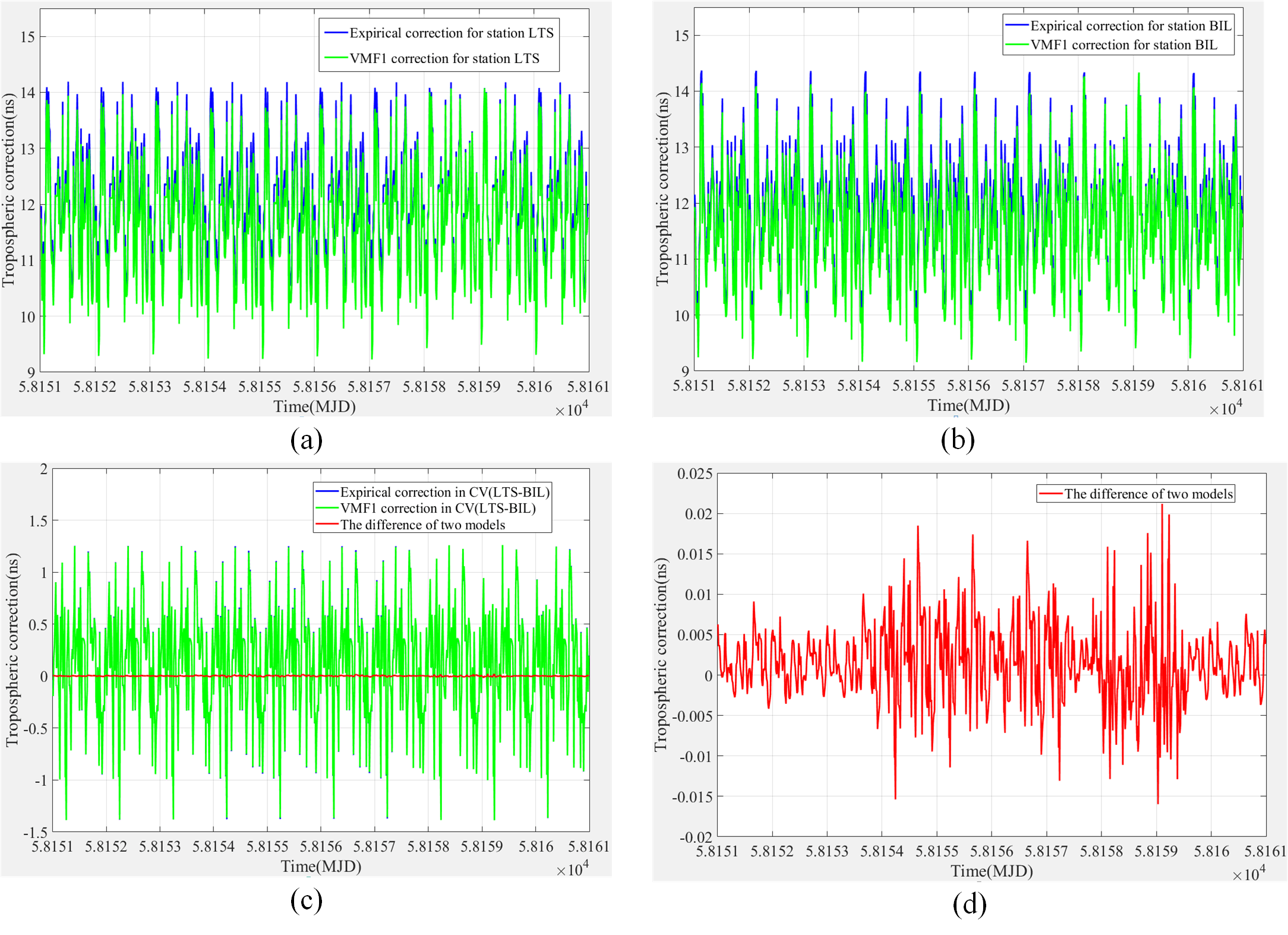
In order to verify the accuracy of the empirical model, we take the two stations (BIL and LTS) from MJD 58151 to 58160 into calculation. We use VMF1 as a comparison, and compare the correction magnitude of the two models in CVSTT technique. The results are shown in Fig. 3, the elevation set-off in our experiment is . From Fig. 3, we conclude that the correction magnitude is tens of nanoseconds for individual stations, and about 2 ns for the two stations via CVSTT technique. And the difference between empirical model and VMF1 is quite small for CVSTT technique (less than 0.025 ns). Therefore, the empirical model is precise enough in our study. In our experiments, after using empirical model for tropospheric correction, the accuracy of the correction achieves 0.52 ns (see Table 1).
3.2.4 Sagnac effect
The Sagnac effect is caused by the rotation of the Earth. During the signal propagation from satellite to station , the Sagnac effect (correction) is expressed as (Ashby,, 2004; Tseng et al.,, 2011; Yang et al.,, 2012):
| (21) |
where is the Earth rotation rate, with a relative uncertainty of (Groten,, 2000).
Taking station A and station B into considertion, the corrections of signal delay of the total Sagnac effect via CVSTT technique can be expressed as follows:
| (22) |
And the accuracy of Sagnac corrections via CVSTT technique can be determined through error propagation law, which is expressed as:
| (23) |
Taking the coordinates of BIL and LTS into consideration, results show that will not exceed 0.003 ns.
| Error type | Sources errors | CVSTT accuracy(ns) | OH accuracy(m) |
|---|---|---|---|
| code noise | 0.97 ns | 4.09 | 43.42 |
| Broadcast ephemeris | 2 m | 0.16 | 1.70 |
| Ground station | 3 cm | 0.15 | 1.60 |
| Ionosphere | - | 0.80 | 8.50 |
| Troposphere | - | 0.52 | 5.52 |
| Sagnac | 0.003 | 0.04 | |
| Total | - | 4.21 | 44.70 |
4 Data processsing method
4.1 EEMD technique
Previous studies (Shen and Ding,, 2014) demonstrates that the ensemble empirical mode decomposition (EEMD) (Wu and Huang,, 2009) is an effective technique for isolating target signals from environmental noises. The EEMD technique is developed from the empirical mode decomposition (EMD) (Huang et al.,, 1998) (https://royalsocietypublishing.org/doi/pdf/10.1098/rspa.1998.0193). The signals series are decomposed into a series of Intrinsic Mode Functions (IMFs) and a residual trend after EEMD decomposition. These IMFs series that are sifted stage by stage reflect local characteristics of the signals, while the residual trend series reflects slow change of the signals (Zhu et al.,, 2013). The specific steps of EEMD are stated as follows (Wu and Huang,, 2009) (https://www.worldscientific.com/doi/abs/10.1142/S1793536909000047):
1) The overall signal series is determined after adding Gaussian white noise into original signal series :
| (24) |
2) The EMD method is applied to implement decomposition for subsequently, these IMFs are determined as:
| (25) |
where denotes IMFj and denotes the residual trend.
3) Adding different Gaussian white noise into and repeating step 1) and step 2), a series of and are determined:
| (26) |
4) According to zero mean principle of Gaussian white noise, the interference cuased by Gaussian white noise can be cancelled after averaging.Therefore, the IMF series can be determined as:
| (27) |
Finally, the original signal series is decomposed into a series of IMFs series and a residual trend series by EEMD technique:
| (28) |
After EEMD decomposition of the signal series , the index of the orthogonality (IO) is calculated to check the completeness of the decomposition, which is defined as follows (Huang et al.,, 1998):
| (29) |
where is defined as:
| (30) |
If the decomposition is completely orthogonal, the cross terms in the right-hand side of expression (29) should be zero, namely IO; and for the worst case IO.
4.2 Simulation experiments
Here, using a simulation experiments we explain the advantages of the EEMD technique. Suppose we have a synthetic series that consists of 3 periodic signals series,(units:ns), where , , Hz, Hz, Hz, respectively, and a linear signal series, , with a data length of 10 days and sampling interval 960 seconds. The can be expressed as:
| (31) |
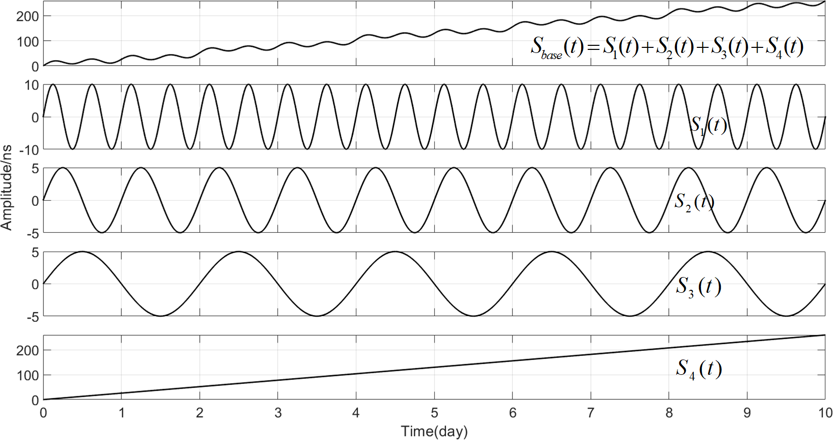
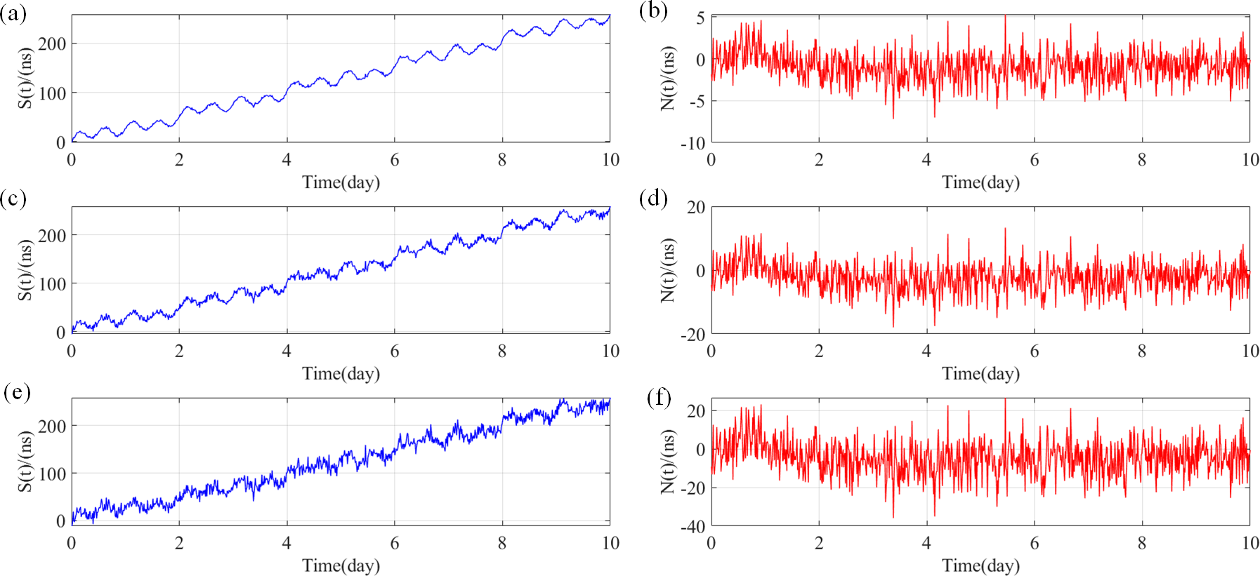
The results of the constructed series are shown in Fig. 4. We added noise signals into with 2 (Case 1), 5 (Case 2) and 10 (Case 3) of the standard deviation (STD) of , and then construct a signal series which contains noise. The can be expressed as:
| (32) |
where the is added noise, which consists of five types of noises, expressed as (Li and Sun,, 2011; Zhai et al.,, 2012; Ashby,, 2015):
| (33) |
where is the white noise phase modulation (W-PM), is the flicker noise phase modulation (F-PM), is the white noise frequency modulation (W-FM), is the flicker noise frequency modulation (F-FM), is the random walk noise frequency modulation (RW-FM).
The constructed signal series with different noise magnitudes are shown in Fig. 5. For our present purpose, the linear signal series is the target signal which need to be extracted from the synthetic signals series .
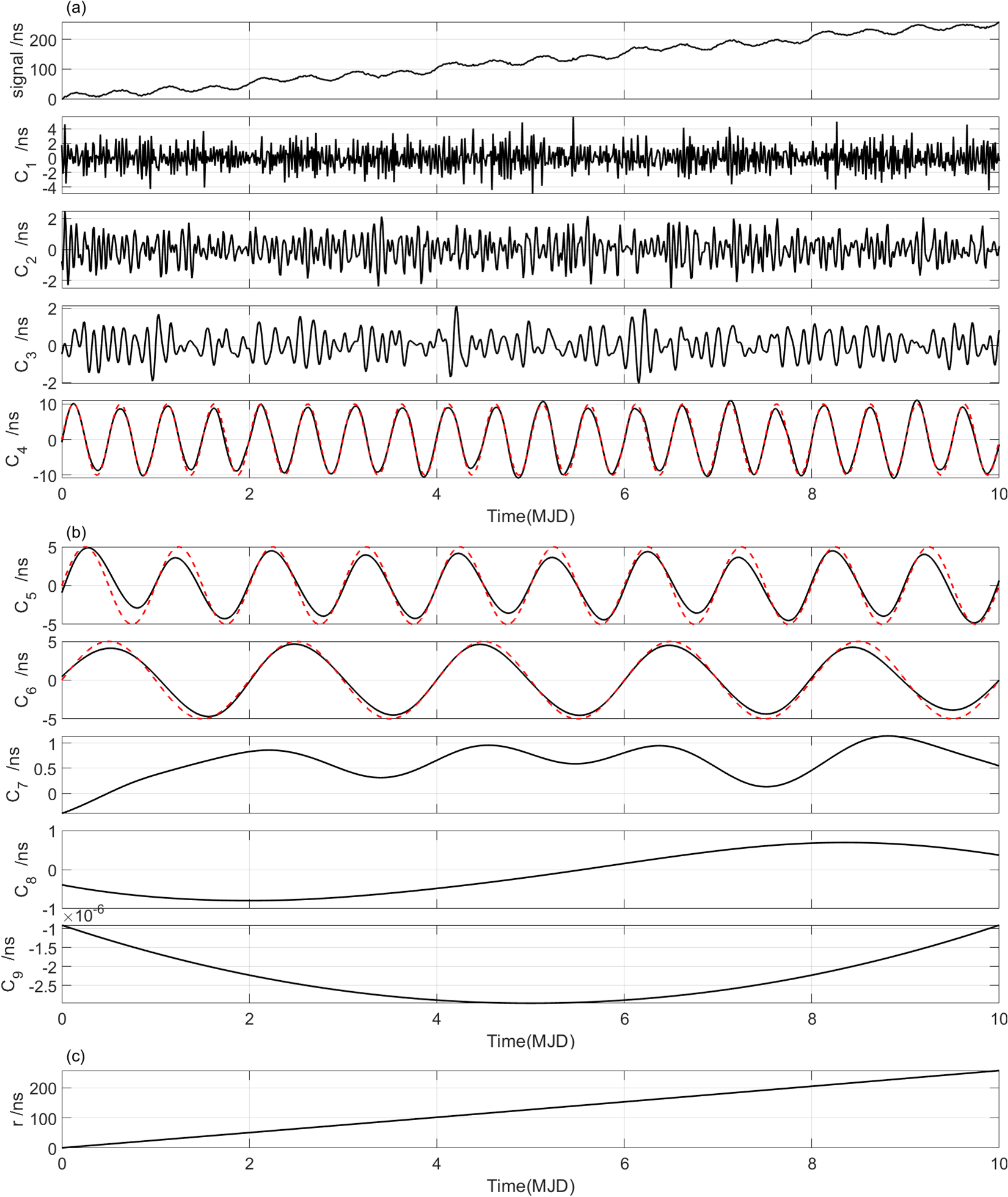
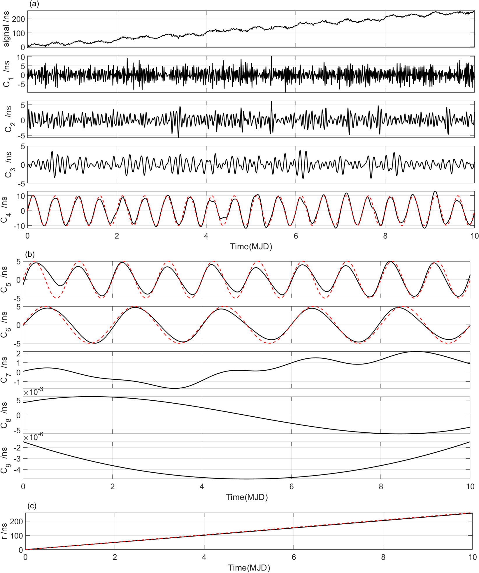
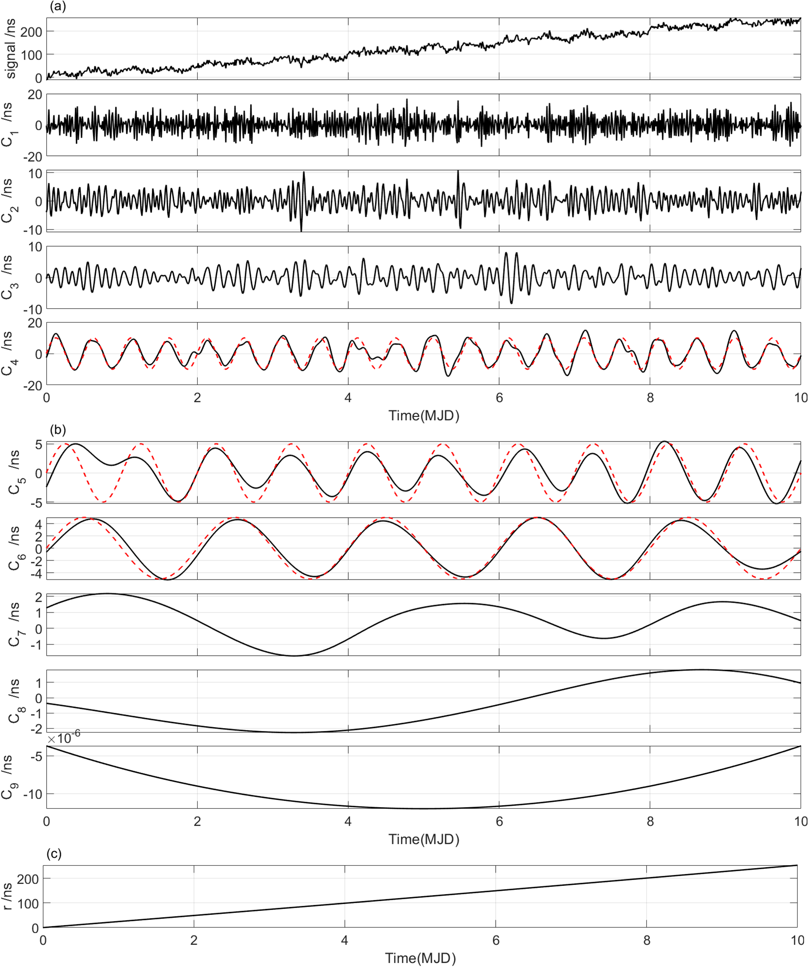
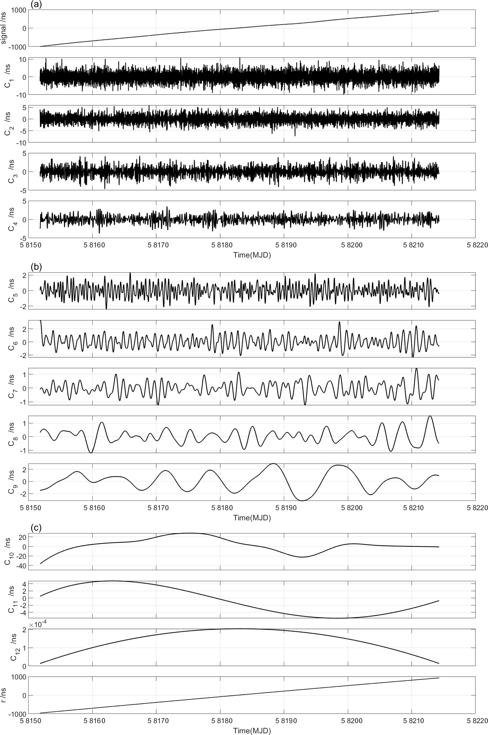
The EEMD technique is applied to identify the periodic signals , and from . After EEMD decomposition, we use the index IO to check completeness of the decomposition. In our simulation experiments, the values of IO are 0.0015 (Case 1), 0.0017 (Case 2) and 0.0017 (Case 3), respectively, suggesting that signal series are effectively decomposed in three different cases. The decomposed IMFs are shown in Figs. 6-8, and we found that the periodic signals , and can be clearly identified, respectively. The red dotted curves in Figs. 6-8 denote the original signals ( = 1, 2, 3) for comparison purpose.
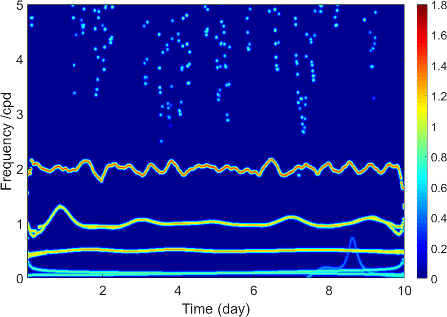
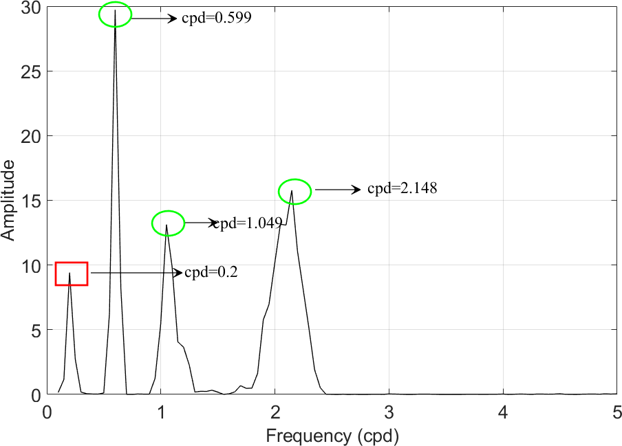
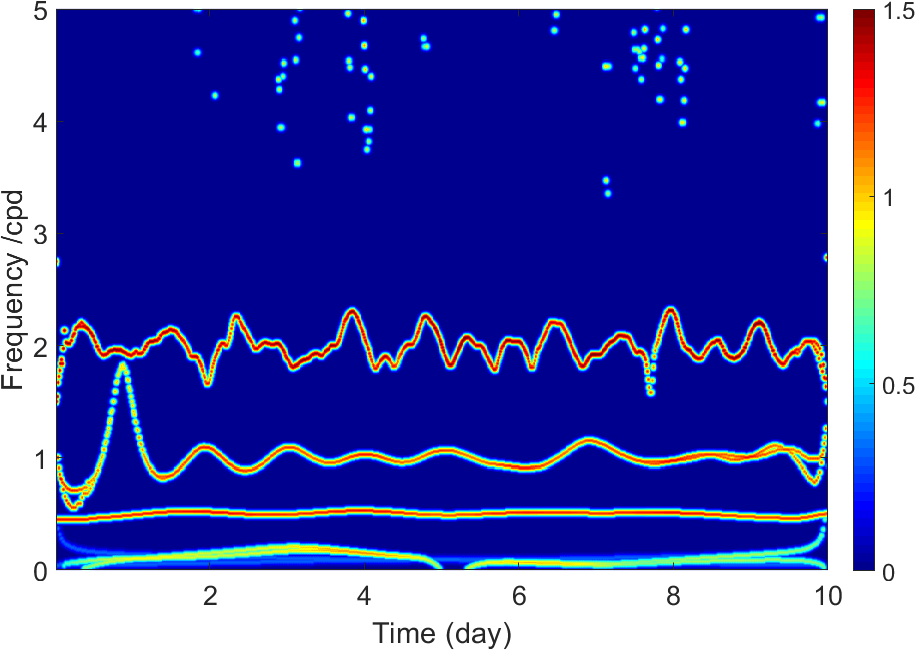
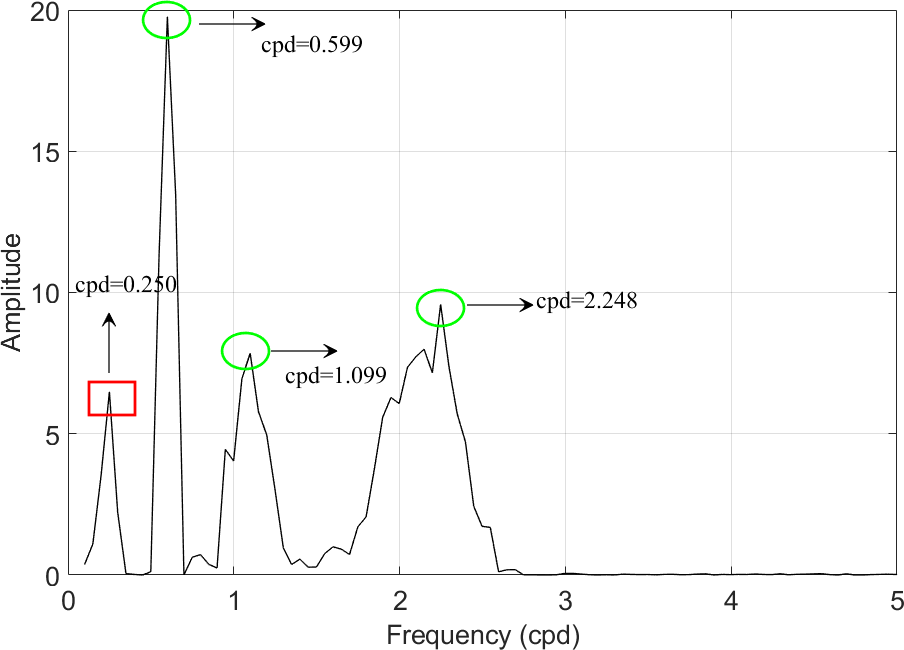
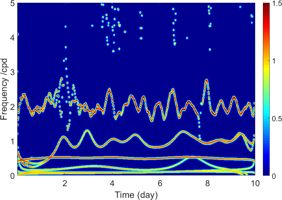
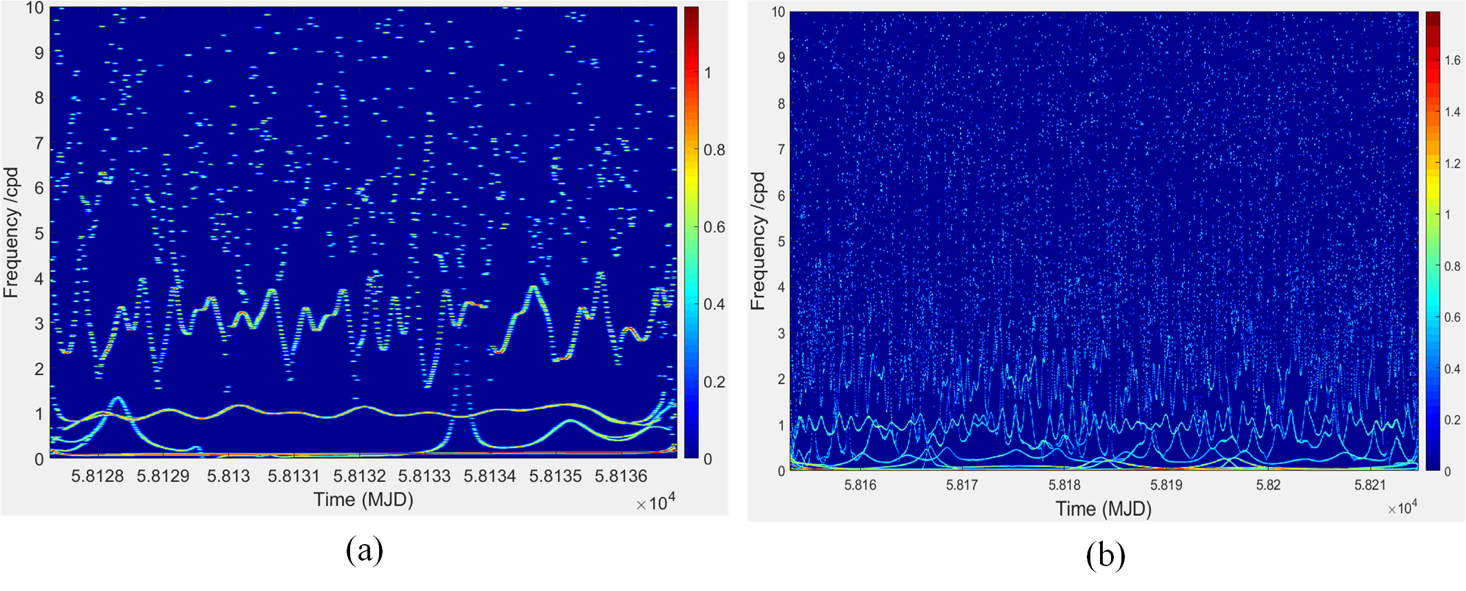
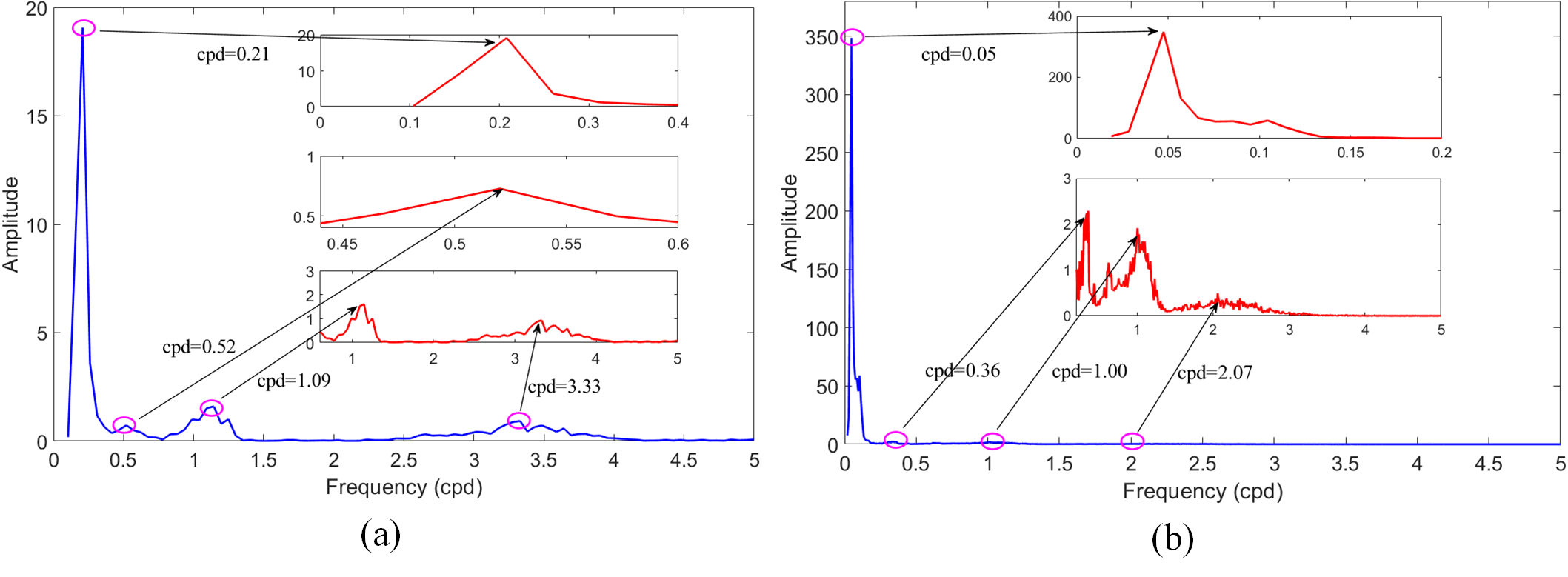
Further, the Hilbert transform (HT) is executed to display the variety of instantaneous frequencies for each IMF component. The corresponding Hilbert spectra and marginal spectra for IMFs (expect for r) in three cases are shown in Figs. 9-11, where each of the subfigures (a)s shows the frequency variations of each IMF, and each of the subfigures (b)s shows measures of the total amplitude (or energy) contribution from each frequency value, representing the cumulated amplitude over the entire data span in a probabilistic sense (Huang et al.,, 1998).
From Figs. 9-11, we see that the mode-mixing problem exists in EEMD decomposition, and it becomes more obvious as noise increases from 2 to 10. However, the three periodic signals , , and can be identified clearly. The set frequencies of , , and are 2 circle per day (cpd), 1 cpd and 0.5 cpd, respectively, denoted as cpd, cpd, and cpd. After EEMD decomposition, the marginal spectra show that the corresponding values are cpd, cpd, cpd (Case 1); cpd, cpd, cpd (Case 2); cpd, cpd, cpd (Case 3), respectively. And the detected signals corresponding to the original set signals , and are shown by the peaks denoted in green circles. In addition, there appear not-real signals with frequencies around 0.2 cpd after EEMD decomposition, which are denoted as and shown by the peaks denoted in red rectangle. The might be meaningless in physical explaining, and it will be an interference if we focus on periodic signals. In this study, however, the target is to detect and identify the linear signal , which means that all periodic signals are useless and should be removed. After all these periodic signals are removed, we reconstruct a new signal series by summing the residual IMFs and the residual trend r. The reconstructed signal series is denoted as .

We take the signal series as real signal series, and try to recovery it by two different methods. The first method is to perform a least squares linear fitting on the signal series directly; and the second method is to perform EEMD decomposition on and then reconstruct the new signal series by removing periodic series IMFs, and the least squares linear fitting is performed on . The results are shown in Fig. 12.
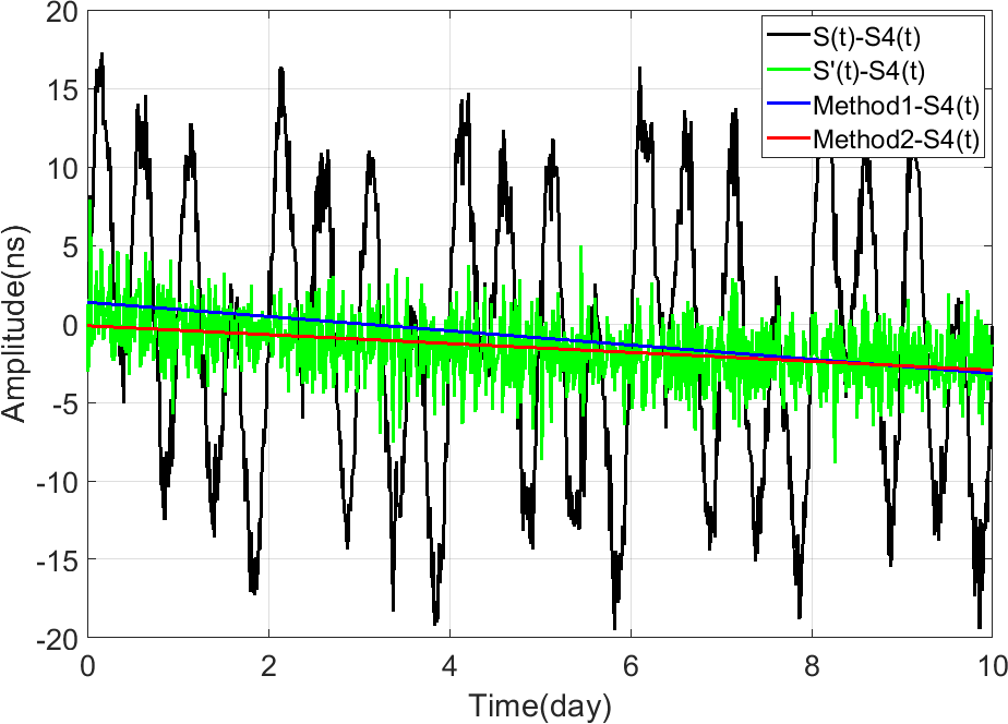
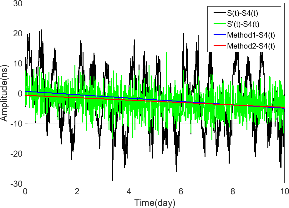
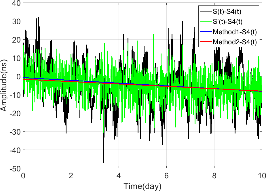
Here we use the standard deviation (STD) of the difference series between the real signal series and that determined by Method 1 or 2 to evaluate the reliability of the two methods. Using Method 1, namely the direct least squared linear fitting of the series , the STDs of the results are 1.31 ns (Case 1), 1.63 ns (Case 2), and 2.16 ns (Case 3), respectively. Using Method 2, namely the least squared linear fitting of the reconstructed series , which is obtained after removing the periodic series via EEMD technique, the STDs of the results are 0.82 ns (Case 1), 1.16 ns (Case 2), and 1.87 ns (Case 3), respectively. The comparative results clearly suggest that the EEMD technique is effective for extracting the linear signals of interest by a priori removing the contaminated periodic signals from the original observations.
5 Experiments and data processing
5.1 Experiments setup
In our experiments, we used two hydrogen time and frequency standards, with one is a fixed reference clock (iMaser3000) and the other is a portable clock (BM2101-02). The experiments are conducted at Beijing 203 Institute Laboratory (BIL) and Luojiashan Time-Frequency Station (LTS), and the locations of the two stations are shown in Fig. 13 and Table 2. And we used the Modified Allan deviation (MDEV)(Allan et al.,, 1991) to evaluate the frequency stability of the two hydrogen atomic clocks, which is estimated from a set of frequency measurements for time averaging. The MDEV is expressed as follows (Allan et al.,, 1991; Bregni and Tavella,, 1997; Lesage and Ayi,, 2007):
| (34) |
where denotes the total number of the time series, denotes the basic time interval, and .
The frequency stabilities of the two clocks on the different average time intervals are given in Table 3. The MDEV with shorter interval represents random noise of the clock, while with longer interval represents secular frequency drift (Kopeikin et al.,, 2016).
| Stations | |||||
|---|---|---|---|---|---|
| BIL | 116.26 | 39.91 | |||
| LTS | 114.36 | 30.53 |
| Time interval | 1 s | 10 s | 100 s | 1000 s | 10000 s |
|---|---|---|---|---|---|
The experiments are divided into two Periods (shown in Fig. 14). In Period 1 that spans from January 09, 2018 to January 29, 2018, the zero-baseline measurement is implenented at BIL with clocks and are placed in the same shielding room with the same geopotentials. According to the International GNSS Tracking Schedule (Allan and Thomas,, 1994; Defraigne and Petit,, 2015), the clock comparisons between and , , are conducted via CVSTT technique, and a series of clock offsets can be obtained, where , and .
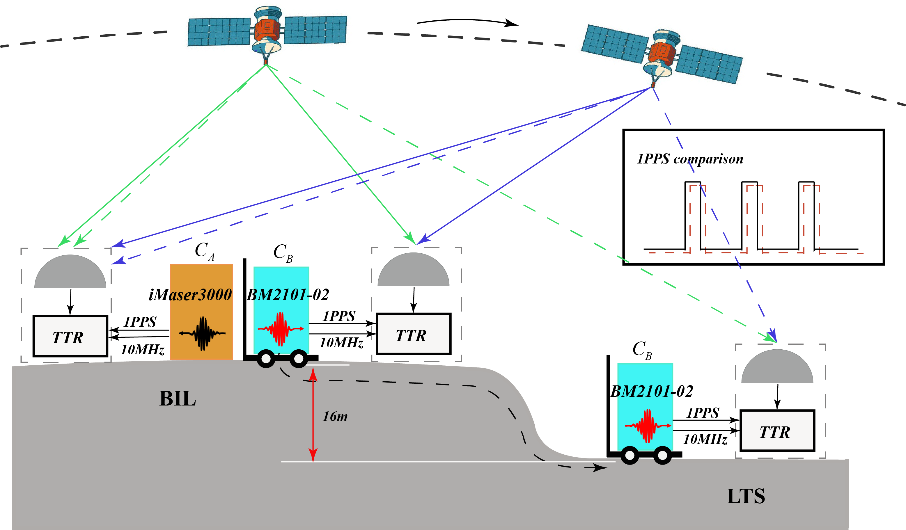
When zero-baseline measurement is finished, the portable clock is transported to LTS from BIL while keeps clock unmoved at the BIL, and during transportation the portable clock continues operating. After installation and adjustment of at the LTS, the clock comparisons between and are conducted in geopotential difference measurement, similarly. And this period is denoted as Period 2, which spans from Febrary 01, 2018 to April 07, 2018. It should be noted that there is no difference except for the location diversity of clock , when comparing the setup difference of Period1 and Period 2. In addition, there are two days of missing data (from January 30, 2018 to January 31, 2018) due to the fact that during transportation (around 8 h) there are no observations and the observations from the day after the re-observation are not stable and consequently not used.
Due to the fact that temperature is a major factor which may disturb the performance of atomic clocks as well as the cable delays (Weiss et al.,, 1999; Lisowiec and Nafalski,, 2004),we controll the environment with a relatively constant temperature in whole experiments. The temperature is held nearly constant ( ) for the fixed clock in Period 1 and Period 2 at BIL. For the portable clock , it is in the same laboratory with clock during Period 1, and the temperature is locked at in Period 2 at LTS.
5.2 Data Processing
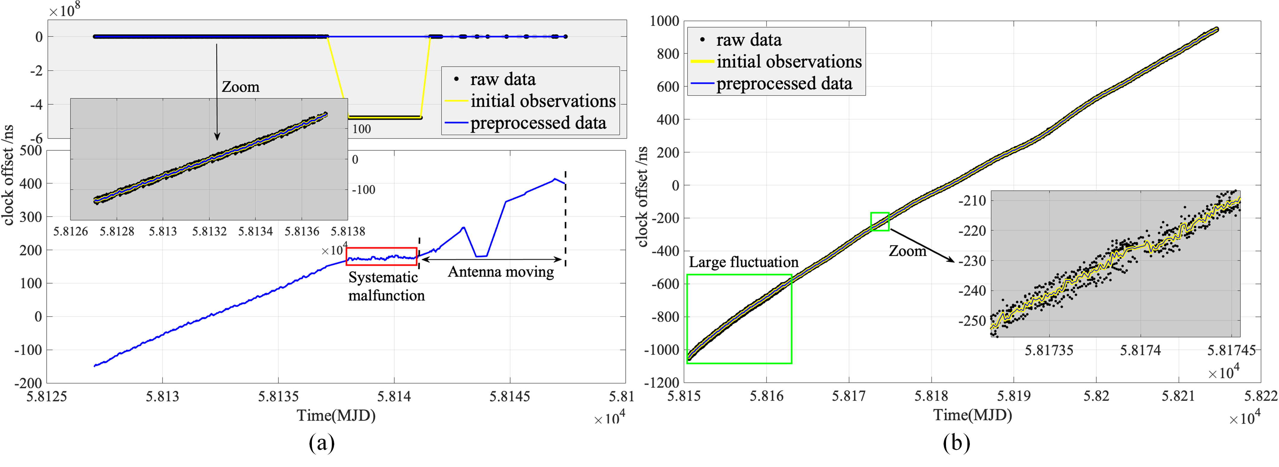
Based on the observations via CVSTT technique, the clock offsets series in each Period are determined. Here, the clock offsets series of the observations for all common-view satellites during Period 1 and Period 2 are denoted by the black dotted curve (simply denoted as raw data) in Fig. 15. And take the satellite elevation angles into consideration, the initial CVSTT observations (initial observations) are obtained, which are denoted by the yellow curve in Fig. 15. After that, we performe data preprocessing on the initial observations by removing gross error, correcting clock jumps and inserting missing data, and the preprocessed CVSTT data (preprocessed data) are finally obtained which denoted by the blue curve in Fig. 15. After data preprocessing, the clock offsets series become more stable. In the following data processing, all operations are based on the preprocessed data sets.
At the same time, it should be noted that, however, the observations from MJD 58137 to MJD 57141 are not used due to a systematic malfunction, and the observations from MJD 58142 to MJD 57147 are also not used due to random movement of the GNSS antenna (the two clocks are not transported, but one antenna is replaced). Therefore, the valid observations in Period 1 spans from MJD 58127 to MJD 57136 (seen in Fig. 15(a)). In Period 2, since the stability of clock could be significantly influenced by various environment factors during its transportation to LTS from BIL, the initial observations at LTS contains large fluctuations and noises (from MJD 58150 to 58161, seen in Fig. 15(b) and Fig. 20(b)), which will contaminate final determination of the geopotentials. Hence, as for preprocessed data in Period 2, we adopt two different preprocessed data sets by whether contains the observations of the first 12 days, and the details are shown later.
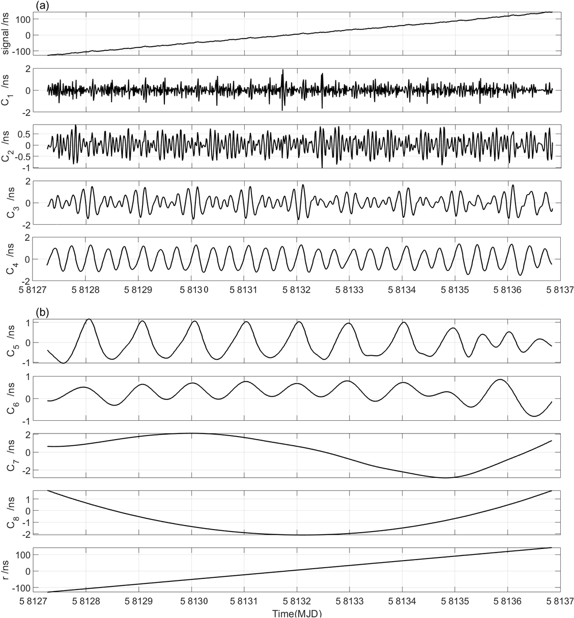
Then, the EEMD technique is applied to the preprocessed data sets for removing the uninteresting periodic components and extracting the geopotential-related signals. The preprocessed data sets in Period 1 and Period 2 are decomposed into a series of IMFs (with frequencies from higher to lower) and a long trend component after EEMD decomposition, as shown in Figs. 16 and 17. Generally, the components of the EEMD convey a physical meaning due to the fact that the characteristic scales are physical (Huang et al.,, 1998). However, the first several high frequency components might be fictitious due to the fact that the sampling interval (960s) is too large to capture the high-frequency variations. As a result, the data are jagged at these frequencies (e.g. in Fig. 16; , , in Fig. 17).
After using EEMD technique for preprocessed data sets in Period 1 and Period 2, we examine completeness and orthogonality of the EEMD decomposition. The IO values corresponding to Period 1 and Period 2 are determined with values of and , respectively, demonstrating that the signals are effectively decomposed. It should be noted that the IO value during Period 2 is worse than that in Period 1. This might be due to the environmental difference of and during Period 2, or due to the difference of the signal propagation paths during Period 2.
The corresponding Hilbert spectra in Period 1 and Period 2 are given in Fig. 18. In order to measure the energy contributions from each frequency value, the marginal spectra of all IMFs are given in Fig. 19, which represent the cumulated amplitude over the entire data span in a probabilistic sense. From Figs. 18 and 19, the periodic signals with frequencies of around 0.2 cpd, 0.5 cpd, 1 cpd and 3.3 cpd of zero-baseline measurement are detected; and the periodic signals with frequencies of around 0.05 cpd, 0.36 cpd, 1 cpd and 2 cpd of geopotential difference measurement are detected. Finally, these periodic signals included in the original CVSTT observation series are removed, and we reconstructed the residual clock offsets series by summing the residual components. The reconstructed clock offsets series are regarded as the geopotential-related signals, based on which we can determine the geopotential difference between (LTS) and (BIL). The reconstructed clock offsets series are denoted as EEMD results, as described in section 4.2.
6 Results
After data processing, the corresponding EEMD results of clock offsets series in Period 1 and Period 2 are determined, as shown in Fig. 20, which provides the clock offsets series before and after EEMD technique via the CVSTT technique. We can find that the clock offsets series become more stable and smooth after removing periodic signals included in the preprocessed data sets. Concerning zero-baseline measurement, after EEMD decomposition and removing periodic IMFs, the EEMD results of the reconstructed clock offsets are determined directly, and the corresponding time elapse difference, , is then determined based on formula (6). We take this result as a system constant shift.
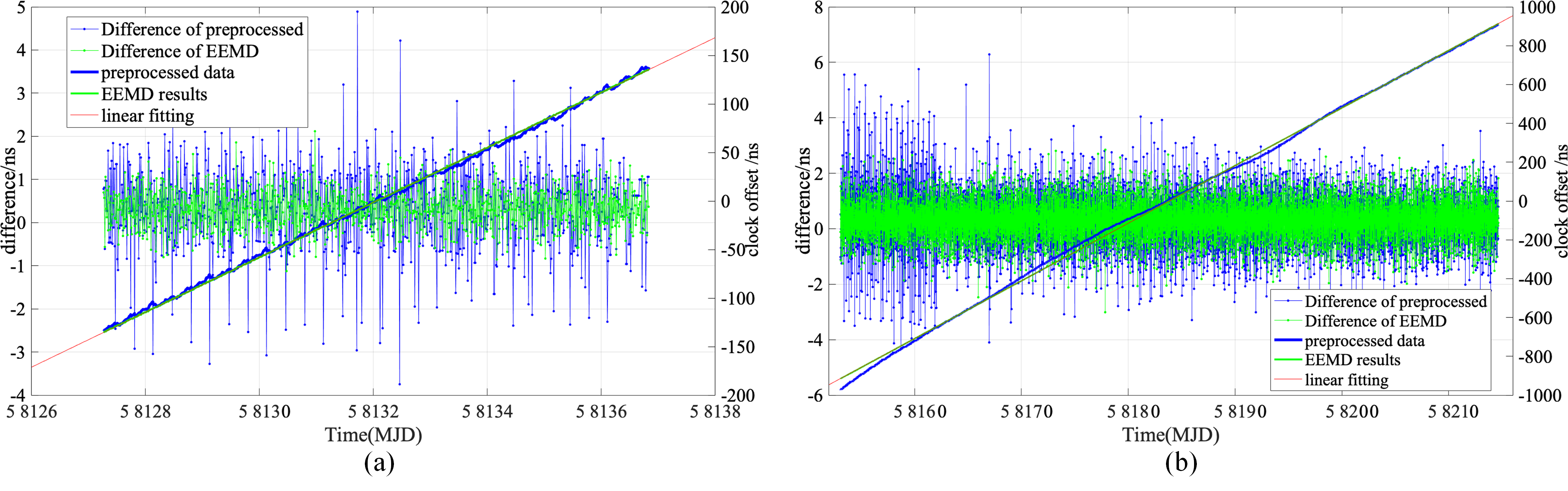
For the geopotential difference measurement, however, the first 12-day observations contain large fluctuations and noises (seen in Fig. 20b) when compared to the later observations. Therefore, the preprocessed data set in Period 2 are analyzed twice. For the first analysis we used the entire data span to implement EEMD decomposition (the red curve in Fig. 21), and for the second analysis we removed the first 12-day observations before EEMD decomposition for avoding data pollution (the green curve in Fig. 21). In addition, for the geopotential difference measurement, we segment the corresponding into 10-day units, not only for matching the zero-baseline duration, but also for improving data utilization. Furthermore, by this strategy, the clock drift could be limited to a relative short time duration (10 days). And we use MDEV of each unit as the weighting factor for determining the final experimental results, which means that for a certain time duration, the higher the stability the greater the weight. By the above strategy, the interference of clock drift could be limited to a relative low level. And based on each unit, a series of time elapse differences are determined.
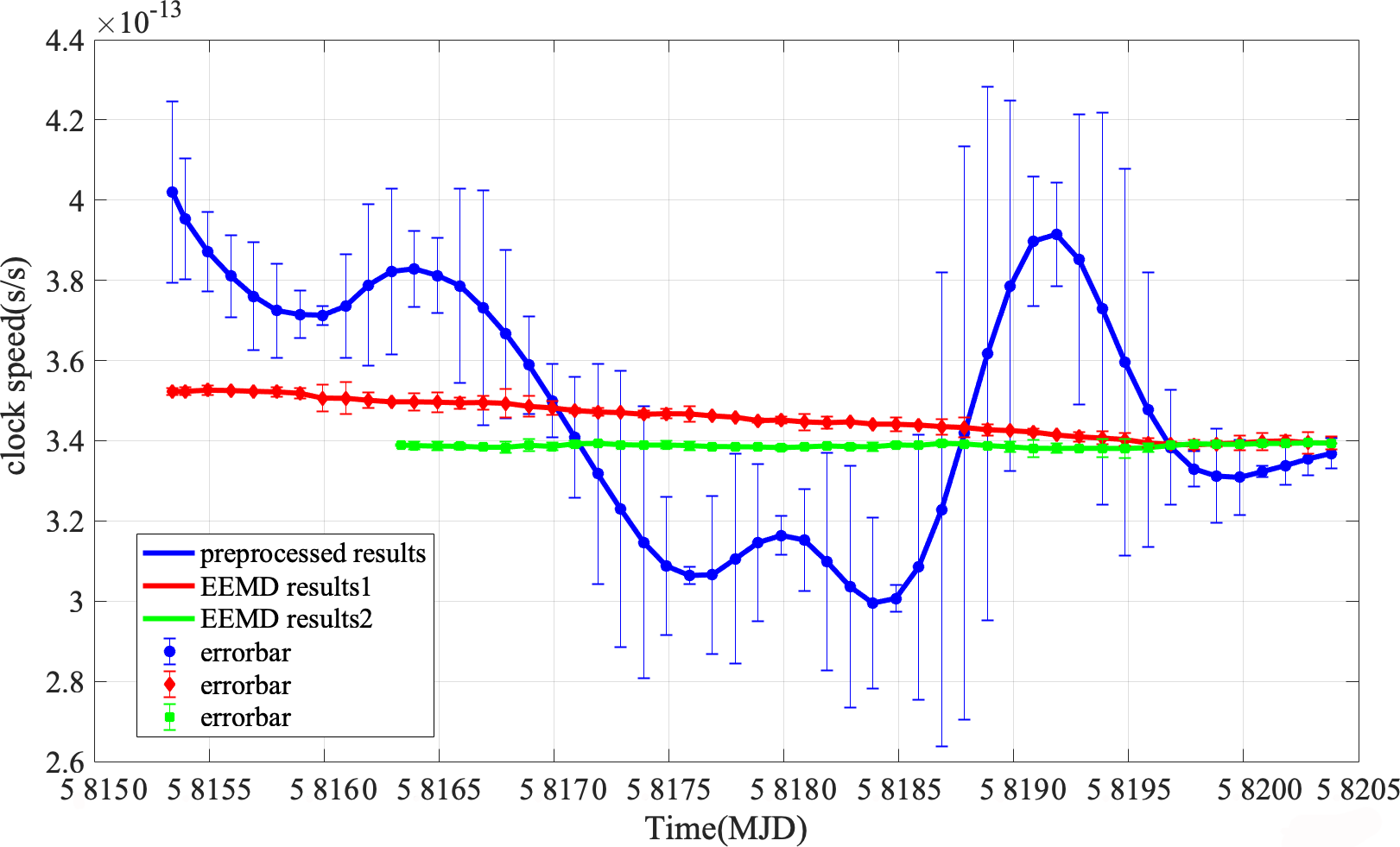
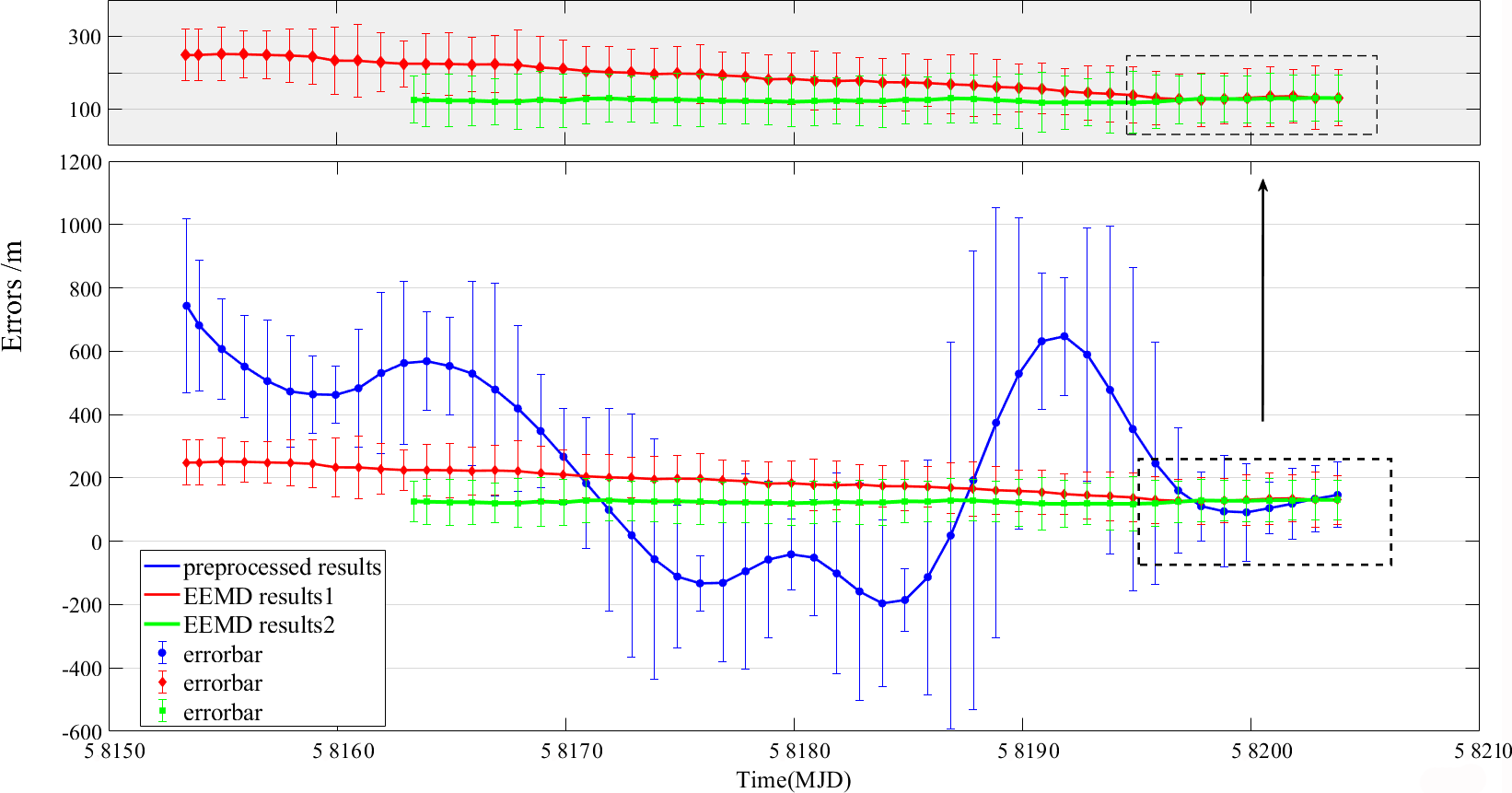
According to equations (2) (6), by taking the results of in Period 1 as system constant shift, the variation of the time elapse difference caused by the geopotentials, is finally determined with . The is caused by the geopotential difference between the two stations and . Therefore, the clock-comparison-determined results of geopotential difference as well as the OH of is obtained. We note that to determine the OH of the station LTS, the OH of the station BIL is a priori given. The results of and are shown in Figs. 21 and 22, respectively. It is noted that the is the discrepancy between the clock-comparison-determined results and the corresponding EGM2008 results . From Figs. 21 and 22, we can find that after removing these periodic signals the results become more stable besides smaller errorbars, which explain the validity of the EEMD technique in extracting the linear signals of interest. In addition, comparing the EEMD results in case 1 (EEMD Results 1) and case 2 (EEMD Results 2), the interference caused by transportation from BIL to LTS is reduced by removing the first 12-days observations in Period 2.
The results of the clock-comparison-determined geopotential difference and OH of clock at LTS are given in Table 6. The results denoted as “preprocessed” and “EEMD” are obtained by taking all measurements in Period 2 as one unit. The results denoted as “M-preprocessed” and “M-EEMD” are obtained by implementing the grouping strategy for the measurements in Period 2 with 10-days measurement as different units, and then we take the mean average of all units as the corresponding final results. The results denoted as “W-preprocessed” and “W-EEMD” are obtained by also implementing the grouping strategy for the measurements in Period 2 with 10-days measurement as different units, and we take the weighted average of all units as the corresponding results. Here we assign weights based on MDEV of each unit, which means that the higher the stability the greater the weight. Due to the fact that the frequency stability of the two hydrogen clocks used in experiments are at the level of /day, the accuracy of the determined geopotential is limited to tens of meters in equivalent height.
Compared to the corresponding EGM2008 model results which suggests that m, the clock-comparison-determined results m. The deviation between the clock-comparison-determined results and the model value is 97.7 m. The results are consistent with the frequency stability of the hydrogen atomic clocks used in our experiments.
| Time span | Strategy | (m) | D(m) | |
|---|---|---|---|---|
| MJD (58150-58215) | ||||
| Preprocessed | ||||
| EEMD | ||||
| M-preprocessed | ||||
| M-EEMD | ||||
| W-preprocessed | ||||
| W-EEMD | ||||
| MJD (58162-58215) | ||||
| Preprocessed | ||||
| EEMD | ||||
| M-preprocessed | ||||
| M-EEMD | ||||
| W-preprocessed | ||||
| W-EEMD |
7 Conclusions
In this study, the clock comparison based on CVSTT technique for determining the geopotential difference is investigated. Based on this approach, one can directly determine the geopotential difference between two ground points. The experimental results provided in Table 6 show that the discrepancy between the clock-comparison-determined result and the corresponding model value is m. This is consistent with the frequency stability of the transportable H-master clocks (iMaser3000 and BM2102-02) used in our experiments.
Here we first used the EEMD technique to remove the periodic signals from the original CVSTT observations to more effectively extract the geopotential-related signals from clock offsets signals. We made comparisons between the results using EEMD and the results without using the EEMD technique, and our study shows that the results using EEMD is better, providing the deviation between the measured OH of the station LTS and the EGM2008 model one with m. We stress that the EEMD technique is applied only to the preprocessing of the observations. If we don’t use it, we still obtain comparable results with m, but a little worse. In addition, as preliminary experiments, we used about 85-days observations to determine the geopotential difference between two stations based on the CVSTT technique, which might be applied extensively in geodesy in the future.
In our present experiments, the residual errors caused by the ionosphere, troposphere, and Sagnac effects can be neglected, for their effects are far below the accuracy level of the hydrogen clocks. However, to achieve centimeter-level measurement accuracy, those influences should be taken into consideration. Namely, more precise correction models need to be considered. In addition, we should use the time-comparison equation accurate to level based on GRT (Kopeikin et al.,, 2011).
With rapid development of time and frequency science and technology, the approach discussed in this study for determining the geopotential difference as well as the OH is prospective and thus, could be implemented as an alternative technique for establishing height datum networks, and has potential applications for unifying the WHS, if GRT holds. Our experimental results are preliminary, and further experiments and investigations are needed to improve the results with high accuracy.
Acknowledgement. We would like to express our sincere thanks to three anonymous reviewers, the responsible editor, and the Editor in Chief of the Journal of Geodesy, for their valuable comments and suggestions, which greatly improved the manuscript. This study was supported by the NSFC (grant Nos. 41721003, 41804012, 41631072, 41874023, 41429401, 41574007) and Natural Science Foundation of Hubei Province of China (grant No. 2019CFB611).
References
- Akatsuka et al., (2008) Akatsuka, T., Takamoto, M., and Katori, H. (2008). Optical lattice clocks with non-interacting bosons and fermions. Nature Physics, 4(12):954–959.
- Allan et al., (1985) Allan, D. W., Davis, D. D., Weiss, M., Clements, A., and Ashby, N. (1985). Accuracy of international time and frequency comparisons via global positioning system satellites in common-view. IEEE Transactions on Instrumentation & Measurement, 34(2):118–125.
- Allan and Thomas, (1994) Allan, D. W. and Thomas, C. (1994). Technical directives for standardization of gps time receiver software. Metrologia, 31(1):69–79.
- Allan and Weiss, (1980) Allan, D. W. and Weiss, M. A. (1980). Accurate time and frequency transfer during common-view of a gps satellite. In Symposium on Frequency Control, pages 334–346.
- Allan et al., (1991) Allan, D. W., Weiss, M. A., and Jespersen, J. L. (1991). A frequency-domain view of time-domain characterization of clocks and time and frequency distribution systems.
- Ashby, (2004) Ashby, N. (2004). The Sagnac Effect in the Global Positioning System.
- Ashby, (2015) Ashby, N. (2015). Probability distributions and confidence intervals for simulated power law noise. IEEE transactions on ultrasonics, ferroelectrics, and frequency control, 62:116–28.
- Bassiri and Hajj, (1993) Bassiri, S. and Hajj, G. A. (1993). Higher-order ionospheric effects on the gps observables and means of modeling them. Advances in the Astronautical Sciences, 18.
- Bjerhammar, (1985) Bjerhammar, A. (1985). On a relativistic geodesy. Bulletin Géodésique, 59(3):207–220.
- Bloom et al., (2014) Bloom, B. J., Nicholson, T. L., Williams, J. R., Campbell, S. L., Bishof, M., Zhang, X., Zhang, W., Bromley, S. L., and Ye, J. (2014). An optical lattice clock with accuracy and stability at the 10(-18) level. Nature, 506(7486):71–5.
- Boehm and Schuh, (2004) Boehm, J. and Schuh, H. (2004). Vienna mapping functions in vlbi analyses. Geophys.res.lett, 31(1):195–196.
- Boehm et al., (2006) Boehm, J., Werl, B., and Schuh, H. (2006). Troposphere mapping functions for gps and very long baseline interferometry from european centre for medium-range weather forecasts operational analysis data. Journal of Geophysical Research: Solid Earth, 111(B2).
- Bondarescu et al., (2015) Bondarescu, M., Bondarescu, R., Jetzer, P., and Lundgren, A. (2015). The potential of continuous, local atomic clock measurements for earthquake prediction and volcanology. page 04009.
- Bondarescu et al., (2012) Bondarescu, R., Bondarescu, M., Hetényi, G., Boschi, L., Jetzer, P., and Balakrishna, J. (2012). Geophysical applicability of atomic clocks: direct continental geoid mapping. Geophysical Journal International, 191(1):78–82.
- Bregni and Tavella, (1997) Bregni, S. and Tavella, P. (1997). Estimation of the percentile maximum time interval error of gaussian white phase noise. In IEEE International Conference on Communications, 1997. ICC ’97 Montreal, Towards the Knowledge Millennium, pages 1597–1601 vol.3.
- Campbell et al., (2017) Campbell, S. L., Hutson, R. B., Marti, G. E., Goban, A., Darkwah, O. N., Mcnally, R. L., Sonderhouse, L., Robinson, J. M., Zhang, W., and Bloom, B. J. (2017). A fermi-degenerate three-dimensional optical lattice clock. Science, 358(6359):90–94.
- Chen et al., (2012) Chen, Q., Song, S., and Zhu, W. (2012). An analysis for the accuracy of tropospheric zenith delay calculated from ecmwf/ncep data over asia. Chinese Journal of Geophysics, 55(3):275–283.
- Dawidowicz and Krzan, (2014) Dawidowicz, K. and Krzan, G. (2014). Coordinate estimation accuracy of static precise point positioning using on-line ppp service, a case study. Acta Geodaetica Et Geophysica, 49(1):37–55.
- Defraigne and Baire, (2010) Defraigne, P. and Baire, Q. (2010). Combining gps and glonass for time and frequency transfer. In Joint Conference of the IEEE International Frequency Control & the European Frequency & Time Forum.
- Defraigne and Baire, (2011) Defraigne, P. and Baire, Q. (2011). Combining gps and glonass for time and frequency transfer. Advances in Space Research, 47(2):265–275.
- Defraigne and Bruyninx, (2007) Defraigne, P. and Bruyninx, C. (2007). On the link between gps pseudorange noise and day-boundary discontinuities in geodetic time transfer solutions. 11(4):239–249.
- Defraigne and Petit, (2015) Defraigne, P. and Petit, G. (2015). Cggtts-version 2e : an extended standard for gnss time transfer. Metrologia, 52(6):G1–G1.
- Deng et al., (2015) Deng, L., Jiang, W., Zhao, L. I., and Peng, L. (2015). Analysis of higher-order ionospheric effects on reference frame realization and coordinate variations. Geomatics & Information Science of Wuhan University, 40(2):193–198.
- Deschenes et al., (2015) Deschenes, J. D., Sinclair, L. C., Giorgetta, F. R., Swann, W. C., Baumann, E., Bergeron, H., Cermak, M., Coddington, I., and Newbury, N. R. (2015). Synchronization of distant optical clocks at the femtosecond level. Physics, 16(1):519–530.
- Einstein, (1915) Einstein, A. (1915). Die feldgleichungen der gravitation. Sitzungsberichte der Koniglich Preußischen Aka-demie der Wissenschaften, 1:844–847.
- Feng et al., (2006) Feng, Y., Moody, M., and Zheng, Y. (2006). Regional gnss satellite orbit monitoring for improved near real-time zenith tropospheric delay estimation. In Dempster, A., editor, Proceedings of the International Global Navigation Satellite Systems Society IGNSS Symposium 2006, pages 1–16, Australia, Queensland, Surfers Paradise. Menay Pty Ltd.
- Gao, (2004) Gao, Y. P. (2004). Use of igs products in gps common view. Acta Astronomica Sinica, 45(1-2).
- Groten, (2000) Groten, E. (2000). Parameters of common relevance of astronomy, geodesy, and geodynamics. JOURNAL OF GEODESY, 74(1):134–140.
- Grotti et al., (2018) Grotti, J., Koller, S., Vogt, S., Häfner, S., Sterr, U., Lisdat, C., Denker, H., Voigt, C., Timmen, L., Rolland, A., Baynes, F., Margolis, H., Zampaolo, M., Thoumany, P., Pizzocaro, M., Rauf, B., Bregolin, F., Tampellini, A., Barbieri, P., and Calonico, D. (2018). Geodesy and metrology with a transportable optical clock. Nature Physics, 14.
- Harmegnies et al., (2013) Harmegnies, A., Defraigne, P., and Petit, G. (2013). Combining gps and glonass in all-in-view for time transfer. Metrologia, 50(3):277–287.
- Heiskanen and Moritz, (1967) Heiskanen, W. A. and Moritz, H. (1967). Physical geodesy. Bulletin Géodésique, 86(1):491–492.
- Hinkley et al., (2013) Hinkley, N., Sherman, J. A., Phillips, N. B., Schioppo, M., Lemke, N. D., Beloy, K., Pizzocaro, M., Oates, C. W., and Ludlow, A. D. (2013). An atomic clock with 10(-18) instability. Science (New York,N.Y.), 341(6151):1215–1218.
- Huang et al., (1998) Huang, N. E., Shen, Z., Long, S. R., Wu, M. C., Shih, H. H., Zheng, Q., Yen, N. C., Chi, C. T., and Liu, H. H. (1998). The empirical mode decomposition and the hilbert spectrum for nonlinear and non-stationary time series analysis. Proceedings of the Royal Society A Mathematical Physical & Engineering Sciences, 454(1971):903–995.
- Huang and Defraigne, (2016) Huang, W. and Defraigne, P. (2016). Beidou time transfer with the standard cggtts. IEEE Transactions on Ultrasonics Ferroelectrics & Frequency Control, 63(7):1005–1012.
- Imae et al., (2004) Imae, M., Suzuyama, T., and Hongwei, S. (2004). Impact of satellite position error on gps common-view time transfer. Electronics Letters, 40(11):709–710.
- Jekeli, (2000) Jekeli, C. (2000). Heights, the geopotential, and vertical datums. Ohio State University.
- Koller et al., (2016) Koller, S. B., Grotti, J., Vogt, S., Almasoudi, A., Dörscher, S., Häfner, S., Sterr, U., and Lisdat, C. (2016). A transportable optical lattice clock with uncertainty. Physical Review Letters, 118(7).
- Kopeikin et al., (2011) Kopeikin, S. M., Efroimsky, M., and Kaplan, G. (2011). Relativistic Celestial Mechanics of the Solar System.
- Kopeikin et al., (2016) Kopeikin, S. M., Kanushin, V. F., Karpik, A. P., Tolstikov, A. S., Gienko, E. G., Goldobin, D. N., Kosarev, N. S., Ganagina, I. G., Mazurova, E. M., and Karaush, A. A. (2016). Chronometric measurement of orthometric height differences by means of atomic clocks. Gravitation & Cosmology, 22(3):234–244.
- Kopeikin et al., (2018) Kopeikin, S. M., Vlasov, I. Y., and Han, W. B. (2018). Normal gravity field in relativistic geodesy. Physical Review D, 97(4).
- Kouba, (2008) Kouba, J. (2008). Implementation and testing of the gridded vienna mapping function 1 (vmf1). Journal of Geodesy, 82(4-5):193–205.
- Lee et al., (1990) Lee, C. B., Lee, D., Chung, N. S., Imae, M., Miki, C., Uratsuka, M., and Morikawa, T. (1990). Development of a gps time comparison system and the gps common-view measurements. In Conference on Precision Electromagnetic Measurements, Cpem 90 Digest.
- Lesage and Ayi, (2007) Lesage, P. and Ayi, T. (2007). Characterization of frequency stability: Analysis of the modified allan variance and properties of its estimate. IEEE Transactions on Instrumentation & Measurement, 33(4):332–336.
- Lewandowski et al., (1999) Lewandowski, W., Azoubib, J., and Klepczynski, W. J. (1999). Gps: primary tool for time transfer. Proceedings of the IEEE, 87(1):163–172.
- Lewandowski and Thomas, (1991) Lewandowski, W. and Thomas, C. (1991). Gps time transfer. Proc IEEE, 79(7):991–1000.
- Li and Sun, (2011) Li, Y. and Sun, H. (2011). Simulation of atomic clock noise by computer.
- Li et al., (2008) Li, Z., Ding, W., and Zhao, L. (2008). Error analysis of orbit determined by gps broadcast ephemeris. Journal of Geodesy & Geodynamics, 28(1):50–54.
- Lion et al., (2017) Lion, G., Panet, I., Wolf, P., Guerlin, C., Bize, S., and Delva, P. (2017). Determination of a high spatial resolution geopotential model using atomic clock comparisons. Journal of Geodesy, 91(6):597–611.
- Lisdat et al., (2016) Lisdat, C., Grosche, G., Quintin, N., Shi, C., Raupach, S. M. F., Grebing, C., Nicolodi, D., Stefani, F., Al-Masoudi, A., Dörscher, S., Häfner, S., Robyr, J. L., Chiodo, N., Bilicki, S., Bookjans, E., Koczwara, A., Koke, S., Kuhl, A., Wiotte, F., Meynadier, F., Camisard, E., Abgrall, M., Lours, M., Legero, T., Schnatz, H., Sterr, U., Denker, H., Chardonnet, C., Le Coq, Y., Santarelli, G., Amy-Klein, A., Le Targat, R., Lodewyck, J., Lopez, O., and Pottie, P. E. (2016). A clock network for geodesy and fundamental science. Nature Communications, 7:12443.
- Lisowiec and Nafalski, (2004) Lisowiec, A. and Nafalski, L. (2004). Progress in temperature stabilization of gps antennas.
- Liu et al., (2017) Liu, X., Shi, M., You, Y., Chuan, L. I., and Rongpan, X. U. (2017). Error analysis of orbit determined by gps/glonass/bds broadcast ephemeris. Science of Surveying & Mapping.
- Mai and Müller, (2013) Mai, E. and Müller, J. (2013). General remarks on the potential use of atomic clocks in relativistic geodesy. ZFV - Zeitschrift fur Geodasie, Geoinformation und Landmanagement, 138(4):257–266.
- Marques et al., (2011) Marques, H. A., Monico, J. F. G., and Aquino, M. (2011). Rinex-ho: second- and third-order ionospheric corrections for rinex observation files. Gps Solutions, 15(3):305–314.
- Mazurova et al., (2017) Mazurova, E., Kopeikin, S., and Karpik, A. (2017). Development of a terrestrial reference frame in the russian federation. Studia Geophysica Et Geodaetica, (27):1–23.
- Mazurova et al., (2012) Mazurova, E., Lapshin, A., and Menshova, A. (2012). Comparison of methods of height anomaly computation. In Egu General Assembly Conference.
- McGrew et al., (2018) McGrew, W. F., Zhang, X., Fasano, R. J., Schäffer, S. A., Beloy, K., Nicolodi, D., Brown, R. C., Hinkley, N., Milani, G., Schioppo, M., Yoon, T. H., and Ludlow, A. D. (2018). Atomic clock performance enabling geodesy below the centimetre level. Nature, 564(7734):87–90.
- Mehlstäubler et al., (2018) Mehlstäubler, T. E., Grosche, G., Lisdat, C., Schmidt, P. O., and Denker, H. (2018). Atomic clocks for geodesy. Reports on Progress in Physics, 81(6):064401.
- Molodenskii, (1962) Molodenskii, M. S. (1962). Methods for study of the external gravitational field and figure of the earth.
- Morton et al., (2009) Morton, Y. T., Zhou, Q., and Herdtner, J. (2009). Assessment of the higher order ionosphere error on position solutions. Navigation, 56(3):185–193.
- Müller et al., (2018) Müller, J., Dirkx, D., Kopeikin, S. M., Lion, G., Panet, I., Petit, G., and Visser, P. N. A. M. (2018). High performance clocks and gravity field determination. Space Science Reviews, 214(1):5.
- Nicholson et al., (2015) Nicholson, T., Campbell, S., Hutson, R., Marti, G., Bloom, B., McNally, R., Zhang, W., Barrett, M., Safronova, M., and Strouse, G. (2015). Systematic evaluation of an atomic clock at total uncertainty. 6:6896.
- Parkingson et al., (1996) Parkingson, B. W., Enge, P., Axelrad, P., and Spilker Jr, J. J. (1996). Global positioning system: Theory and applications, volume i. Progress in Astronautics and Aeronautics, Vols. 1 and 2.
- Pavlis and Weiss, (2017) Pavlis, N. and Weiss, M. (2017). A re-evaluation of the relativistic redshift on frequency standards at nist, boulder, colorado, usa. Metrologia, 54(4).
- Peng and Liao, (2009) Peng, H. M. and Liao, C. S. (2009). Gps smoothed p3 code for time transfer. In Frequency and Time Forum, 2004. Eftf 2004. European, pages 137–141.
- Petit and Arias, (2009) Petit, G. and Arias, E. F. (2009). Use of igs products in tai applications. Journal of Geodesy, 83(3-4):327–334.
- Poli et al., (2014) Poli, N., Schioppo, M., Vogt, S., Falke, S., Sterr, U., Lisdat, C., and Tino, G. M. (2014). A transportable strontium optical lattice clock. Applied Physics B, 117(4):1107–1116.
- Ray and Senior, (2003) Ray, J. and Senior, K. (2003). Igs/bipm pilot project: Gps carrier phase for time/frequency transfer and timescale formation. Metrologia, 40(3):270–288.
- Riehle, (2017) Riehle, F. (2017). Optical clock networks. Nature Photonics, 11(1):25–31.
- Rose et al., (2016) Rose, J. A. R., Watson, R. J., Allain, D. J., and Mitchell, C. N. (2016). Ionospheric corrections for gps time transfer. Radio Science, 49(3):196–206.
- Shen, (1998) Shen, W. (1998). Relativistic Physical Geodesy:[Dissertation]. Graz Technical University, Graz.
- Shen et al., (1993) Shen, W., Chao, D., and Jin, B. (1993). On relativistic geoid. Bollettino di Geodesia e Scienze Affini, 52(3):207–216.
- Shen and Ding, (2014) Shen, W. and Ding, H. (2014). Observation of spheroidal normal mode multiplets below 1 mhz using ensemble empirical mode decomposition. Geophysical Journal International, 196(3):1631–1642.
- Shen et al., (2011) Shen, W., Ning, J., Liu, J., Li, J., and Chao, D. (2011). Determination of the geopotential and orthometric height based on frequency shift equation. Natural Science, 3(5):388–396.
- Shen et al., (2019) Shen, W., Sun, X., Cai, C., Wu, K., and Shen, Z. (2019). Geopotential determination based on a direct clock comparison using two-way satellite time and frequency transfer. Terrestrial, Atmospheric and Oceanic sciences journal, 30(1):1–11.
- (75) Shen, W., Tian, W., and Hou, K. (2009a). An approach for determining the orthometric height using gps signals and the preliminary experimental results.
- (76) Shen, W. B., Ning, J., Chao, D., and Liu, J. (2009b). A proposal on the test of general relativity by clock transportation experiments. Advances in Space Research, 43(1):164–166.
- Shen and Shen, (2015) Shen, Z. and Shen, W. (2015). Geopotential difference determination using optic-atomic clocks via coaxial cable time transfer technique and a synthetic test. Geodesy & Geodynamics, 6(5):344–350.
- Shen et al., (2016) Shen, Z., Shen, W., and Zhang, S. (2016). Formulation of geopotential difference determination using optical-atomic clocks onboard satellites and on ground based on doppler cancellation system. Geophysical Journal International, 206(2):ggw198.
- Shen et al., (2018) Shen, Z., Shen, W., Zhao, P., Tao, L., Zhang, S., and Chao, D. (2018). Formulation of determining the gravity potential difference using ultra-high precise clocks via optical fiber frequency transfer technique. Journal of Earth Science, (12):1–7.
- Shen et al., (2017) Shen, Z., Shen, W. B., and Zhang, S. (2017). Determination of gravitational potential at ground using optical-atomic clocks on board satellites and on ground stations and relevant simulation experiments. Surveys in Geophysics, 38(4):757–780.
- Singh et al., (2015) Singh, Y., Smith, L., Origlia, S., Wei, H., Śweirad, D., Hughes, J., Kock, O., Alighanbari, S., Schiller, S., and Kai, B. (2015). Development of a strontium optical lattice clock for space applications. 41.
- Sun et al., (2010) Sun, H., Yuan, H., and Zhang, H. (2010). The impact of navigation satellite ephemeris error on common-view time transfer. IEEE Transactions on Ultrasonics Ferroelectrics & Frequency Control, 57(1):151.
- Sánchez and Sideris, (2017) Sánchez, L. and Sideris, M. G. (2017). Vertical datum unification for the international height reference system (ihrs). Geophysical Journal International, pages 570–586.
- Sánchez et al., (2016) Sánchez, L., Čunderlík, R., Dayoub, N., Mikula, K., Minarechová, Z., Šíma, Z., Vatrt, V., and Vojtíšková, M. (2016). A conventional value for the geoid reference potential (w0). Journal of Geodesy, 90(9):815–835.
- Takano et al., (2016) Takano, T., Takamoto, M., Ushijima, I., Ohmae, N., Akatsuka, T., Yamaguchi, A., Kuroishi, Y., Munekane, H., Miyahara, B., and Katori, H. (2016). Geopotential measurements with synchronously linked optical lattice clocks. Nature Photonics, 10.
- Tseng et al., (2011) Tseng, W. H., Feng, K. M., Lin, S. Y., Lin, H. T., and Liao, C. S. (2011). Sagnac effect and diurnal correction on two-way satellite time transfer. IEEE Transactions on Instrumentation & Measurement, 60(7):2298–2303.
- Weinberg, (1972) Weinberg, S. (1972). General relativity. (book reviews: Gravitation and cosmology. principles and applications of the general theory of relativity).
- Weiss et al., (1999) Weiss, M. A., Ascarunz, F. G., Parker, T., Zhang, V., and Gao, X. (1999). Effects of antenna cables on gps timing receivers. In Frequency & Time Forum, & the IEEE International Frequency Control Symposium, Joint Meeting of the European.
- Wu and Huang, (2009) Wu, Z. and Huang, N. E. (2009). Ensemble empirical mode decomposition: A noise-assisted data analysis method. Advances in Adaptive Data Analysis, 1(01):–.
- Xu, (2007) Xu, G. (2007). GPS: Theory, Algorithms and Applications, 2nd edition by Guochang Xu. Berlin: Springer, 2007.
- Yang et al., (2012) Yang, X., Hu, Z., Guo, J., Li, X., Li, Z., and Yuan, H. (2012). Method of common-view time transfer with transfer mode based on geostationary satellite. In Frequency Control Symposium, pages 1–4.
- Zhai et al., (2012) Zhai, J., Dong, L., Zhang, S., Lu, F., and Hu, L. (2012). Different variances used for analyzing the noise type of atomic clock. Applied Mechanics and Materials, 229-231:1980–1983.
- Zhang et al., (2013) Zhang, X., REN, X., and GUO, F. (2013). Influence of higher-order ionospheric delay correction on static precise point positioning. GEOMATICS AND INFORMATION SCIENCE OF WUHAN UNIVERS, 38(8):883–887.
- Zhu et al., (2013) Zhu, N., Bai, X., and Dong, W. (2013). Harmonic detection method based on eemd. Proceedings of the Csee, 33(7):92–98.