Preventing Exceptions to Robins InEquality
Abstract
For sufficiently large Ramanujan gave a sufficient condition for the truth Robin’s InEquality (RIE). The largest known violation of RIE is . In this paper Robin’s multipliers are split into logarithmic terms and relative divisor sums . A violation of RIE above is proposed to imply oscillations that cause to exceed . To this aim Alaoglu and Erdős’s conjecture for the CA numbers algorithm is used and the paper could almost be reduced to section 4.3 on pages 4.3 to 5.
1 Introduction
1.1 Outline
Robin’s Inequality (RIE) for sufficiently large can be derived from Ramanujan’s Lost Notebook as necessary condition for RH. Unfortunately his work was not published until 1997. The inequality can be derived from an asymptotic expression that emerged from the study of generalised highly composite and generalised superior highly composite numbers. Alaoglu and Erdős coined the terms superabundant (SA) and colossally abundant (CA) in 1944 and mentioned the role of transcendental number theory in the process of finding CA numbers.
Robin clarified the meaning of “sufficiently large” in 1984 by finding
-
1.
that the function takes maximal values on CA numbers.
-
2.
It is sufficient for RH that RIE holds true for sufficiently large , i.e. for .
-
3.
The oscillation theorem in CA numbers if RH is false.
-
4.
has an unconditional bound for some .
The major tool were estimations with Chebyshev’s functions and using the results of Rosser and Schoenfeld. In order to show that takes maximal values on CA numbers Robin used a multiplier consisting of ratios of relative divisor sums of consecutive CA numbers and iterated logarithms. The argument is iterated in this report which proves that takes a greater value on a subsequent CA number if the product of ratios of relative divisor sums of intermediate CA numbers exceeds the respective product of ratios of iterated logarithms. But the CA numbers algorithm relies on the quotient of consecutive CA numbers to be prime which is not guaranteed unless Alaoglu and Erdős’ special case of the Four Exponentials Conjecture is true.
The point of this investigation has been to find out if the minimal oscillations in case RH is false will force the products of ratios of relative divisor sums to become greater than the corresponding products of ratios of iterated logarithms. This has been achieved by finding a template for the quotient of maximal and minimal values of as proceeds in CA numbers and analysing the template with polar coordinates.
The paper is primarily organised as a chain of reductions that is summarised in the final Conclusion 4.32. Section 1.2 establishes the need to find multiples of every natural on which takes a greater value than it takes on . Such multiples prevent from being an exception. Section 2 demonstrates how the multipliers used by Robin work and how they can be split. This method is iterated in Section 3 to show the sufficiency of testing for and . Similar conditions were found in [33, 35, 34] during the course of my investigation. The setup of the latter two reports is summarised using the present setup as a part of section 4 after presenting some numerical data. Then Mertens’ theorem motivates expecting the truth of before Robin’s oscillation theorem is used in section 4.3 to propose an indirect proof.
1.2 Preparation
Notation.
Grönwall [17] mentioned that the asymptotic behaviour of the function had been studied by Landau, [25]. Then he proved Theorem 1.3 below. Rf. [36, 13] for Nicolas’ inequality and [52, 53] for approaches with the Dedekind function. Suppose
Condition 1.1.
For every there is a number such that .
Note.
This section establishes
Claim 1.2.
is true for all .
If the opposite of Condition 1.1 was true for some the number may be said to be exceptional since no such is known so far. Without requiring this is called GA2 in [8, p. 2]. Known GA2 numbers are 3, 4, 5, 6, 8, 10, 12, 18, 24, 36, 48, 60, 72, 120, 180, 240, 360, 2520, and 5040. Recall
Theorem 1.3.
(Grönwall)
This is easily extended.
Theorem 1.4.
Thus, assuming Condition 1.1 it is easily seen that a minimal counterexample of RIE above 5040 contradicts Theorem 1.6 since for any number Condition 1.1 implies the existence of a non-decreasing sequence of values of that starts at . If choose such that
-
1.
for all where and
-
2.
, i.e. .
The contradiction to Theorem 1.6 follows. Thus
Corollary 1.8.
There is no GA2 number . In other words there is no exceptional number.
Proving the absence of exceptional numbers seems to be just as difficult as proving Condition 1.1. This is no surprise because a one is an indirect proof of the other.
2 Colosally Abundant Numbers
Definition 2.1.
By Theorem 1.3 there are infinitely many SA numbers but they are only mentioned here because the SA property suffices to determine the asymptotic behaviour of .
Fact 2.2.
Rf. [37, 38] for more information.
“A superparticular number is when a great number contains a lesser number, to which it is compared, and at the same time one part of it.” Rf. [57, p.III.6.12,n.7].
Notation 2.3.
Definition 2.4.
Let denote the function and Robin’s multiplier be .
Note 2.5.
-
1.
The derivatives of are given by
which implies that is convex for every .
-
2.
as or as since logs grow slower than any power of .
-
3.
If then for all because . In particular and do not intersect if .
-
4.
and .
-
5.
if .
Proof.
Based on this setup the algorithm computing the sequence of CA numbers seems to be well-understood, [39, 3, 16, 46, 40, 37, 7, 38, 13, 8, 9, 51]. Nevertheless there is the open
Question 2.7.
-
1.
Can the algorithm find a new violation of RIE? (Does one exist?)
-
2.
Do two consecutive CA numbers exist whose quotient is semiprime?
Item 2. has been given a negative answer under the following Conjecture, rf. [3, p. 455].
Conjecture 2.8.
(Four Exponentials)
Semiprime quotients cause unexpected difficulties. Therefore I assume a special case of Conjecture 2.8.
Assumption 2.9.
(Alaoglu and Erdős)
For any two distinct prime numbers and , the only real numbers for which both and are rational are the positive integers.
Conclusion 2.10.
is prime for all , rf. [62, Colossally abundant number].
3 Subsequent Maximisers
3.1 Extending Robin’s Method
Definition 3.1.
Let , , , and . Contextually write for or if where . Put .
Fact.
.
Lemma 3.2.
and .
Proof.
By induction on using Lemma 2.5, #4.∎
Corollary 3.3.
If then so for all if but if .
Theorem 3.4.
is exceptional if and only if and .
Proof.
for all iff is exceptional. On the the other hand for all iff and the claim follows with Lemma 3.2.∎
Condition 3.5.
for all .
Condition 3.7.
For every with there is some such that .
3.2 Number Crunching
- 1.
| 4 | 14 | 4 | 5 | 8 | 17 | 24 | |
| 8.5251 | 3274.0 | 10.9230 | 16.889 | 107.7176 | 20432.8 | 1912150.6 | |
| 1.9459 | 8.0885 | 2.3978 | 2.5649 | 4.6151 | 9.9212 | 14.4633 | |
| 1.9356 | 7.8588 | 2.1174 | 2.5342 | 4.3330 | 9.7132 | 14.2938 | |
| 2.1430 | 8.0937 | 2.3908 | 2.8266 | 4.6795 | 9.9249 | 14.4637 | |
| 1 | 33 | 1 | 1 | 1 | 1 | ||
| 3.7024 | 1421.9 | 4.7438 | 7.335 | 46.7811 | 8873.60 | 830436.46 | |
| 0.5684 | 3.1528 | 0.6761 | 0.8654 | 1.6700 | 3.9480 | 5.9193 | |
| 3.8380 | 14.3887 | 4.1870 | 4.8559 | 8.1962 | 17.6663 | 25.7599 | |
| 1.79097 | 1.7777 | 1.7512 | 1.7179 | 1.7515 | 1.7800001 | 1.7810000003 | |
| 1.9047 | 1.79096 | 1.8944 | 1.8621 | 1.8106 | 1.7877 | 1.7842 | |
| 8.0913 | undefined since | ||||||
Theorem 3.8.
For every CA if there is a subsequent CA such that .
Proof.
was confirmed in every loop. (Not shown in Appendix A.) ∎
-
2.
Keith Briggs reported to me: "E.g. the following is a CA number:
with loglog about 26." Denote it by and call the tuple (2, , 3, , 5, , 7, , 11, 13, 17, 23, 37, 53, 101, 239, 887, 7789, 562399, 162216342187) bottom-up form. Since he reached about according to [7, §3]
reveals in compliance with [56, Section 10.1.2] and Fact 2.2. This was significantly more than the theoretically obtained bound from [8, Corollary 1] which my rather short calculation capped, too. Noe’s top-down representation is
Theorem 3.9.
For every CA such that there is a subsequent CA such that .
| 8 | 4 | 2 | 7 | 8.5 | 4 | 31:30 | 1 | 4.73 | 2.143 | 1 | |
| 9 | 4 | 11 | 11 | 10.9 | 1 | 12:11 | 1.090 | 3.62 | 2.390 | 1.115 | 1 |
| 10 | 4 | 13 | 13 | 13.4 | 1 | 14:13 | 1.174 | 2.88 | 2.601 | 1.214 | 1.13 |
| 11 | 5 | 2 | 13 | 14.1 | 5 | 63:62 | 1.193 | 2.31 | 2.651 | 1.237 | 1.48 |
| 12 | 5 | 3 | 13 | 15.2 | 3 | 40:39 | 1.224 | 2.30 | 2.726 | 1.272 | 1.80 |
| 13 | 5 | 5 | 13 | 16.8 | 2 | 31:30 | 1.265 | 2.03 | 2.826 | 1.319 | 2.25 |
| 14 | 5 | 17 | 17 | 19.7 | 1 | 18:17 | 1.339 | 2.01 | 2.981 | 1.391 | 1.91 |
| 15 | 5 | 19 | 19 | 22.6 | 1 | 20:19 | 1.410 | 1.74 | 3.120 | 1.456 | 1.27 |
| 16 | 5 | 23 | 23 | 25.8 | 1 | 24:23 | 1.471 | 1.35 | 3.250 | 1.516 | 1.07 |
| 17 | 6 | 2 | 23 | 26.4 | 6 | 127:126 | 1.483 | 1.12 | 3.276 | 1.529 | 1.11 |
| 18 | 6 | 29 | 29 | 29.8 | 1 | 30:29 | 1.534 | 1.00 | 3.396 | 1.584 | 1.42 |
| 19 | 6 | 31 | 31 | 33.2 | 1 | 32:31 | 1.583 | 9.24 | 3.505 | 1.635 | 1.44 |
| 20 | 6 | 7 | 31 | 35.2 | 2 | 57:56 | 1.612 | 9.09 | 3.562 | 1.662 | 1.22 |
| 21 | 6 | 3 | 31 | 36.3 | 4 | 121:120 | 1.625 | 7.55 | 3.592 | 1.676 | 1.27 |
| 22 | 6 | 37 | 37 | 39.9 | 1 | 38:37 | 1.669 | 7.38 | 3.687 | 1.720 | 1.21 |
| 23 | 6 | 41 | 41 | 43.6 | 1 | 42:41 | 1.710 | 6.48 | 3.776 | 1.762 | 1.19 |
| 24 | 6 | 43 | 43 | 47.4 | 1 | 44:43 | 1.749 | 6.11 | 3.859 | 1.800 | 1.00 |
| 25 | 7 | 2 | 43 | 48.1 | 7 | 255:254 | 1.756 | 5.66 | 3.873 | 1.807 | 9.82 |
| 26 | 7 | 47 | 47 | 51.9 | 1 | 48:47 | 1.794 | 5.46 | 3.950 | 1.843 | 7.75 |
| 27 | 7 | 53 | 53 | 55.9 | 1 | 54:53 | 1.828 | 4.70 | 4.024 | 1.877 | 7.51 |
| 28 | 7 | 59 | 59 | 60.0 | 1 | 60:59 | 1.858 | 4.12 | 4.094 | 1.910 | 8.54 |
| 29 | 7 | 5 | 59 | 61.6 | 3 | 156:155 | 1.870 | 3.99 | 4.121 | 1.923 | 8.61 |
| 30 | 7 | 61 | 61 | 65.7 | 1 | 62:61 | 1.901 | 3.95 | 4.185 | 1.953 | 7.51 |
| 31 | 7 | 67 | 67 | 69.9 | 1 | 68:67 | 1.930 | 3.52 | 4.247 | 1.982 | 7.42 |
| 32 | 7 | 71 | 71 | 74.2 | 1 | 72:71 | 1.957 | 3.28 | 4.306 | 2.009 | 7.25 |
| 33 | 7 | 73 | 73 | 78.4 | 1 | 74:73 | 1.984 | 3.17 | 4.363 | 2.035 | 6.18 |
| 34 | 7 | 11 | 73 | 80.8 | 2 | 133:132 | 1.999 | 3.14 | 4.393 | 2.049 | 4.99 |
| 35 | 7 | 79 | 79 | 85.2 | 1 | 80:79 | 2.024 | 2.87 | 4.445 | 2.074 | 3.79 |
| 36 | 8 | 2 | 79 | 85.9 | 8 | 511:510 | 2.028 | 2.82 | 4.453 | 2.078 | 3.54 |
| 37 | 8 | 83 | 83 | 90.3 | 1 | 84:83 | 2.052 | 2.71 | 4.503 | 2.101 | 2.11 |
| 38 | 8 | 3 | 83 | 91.4 | 5 | 364:363 | 2.058 | 2.50 | 4.516 | 2.107 | 1.98 |
| 39 | 8 | 89 | 89 | 95.9 | 1 | 90:89 | 2.081 | 2.48 | 4.563 | 2.129 | 8.18 |
| 40 | 8 | 97 | 97 | 100 | 1 | 98:97 | 2.103 | 2.24 | 4.610 | 2.151 | 6.26 |
| 41 | 8 | 13 | 97 | 103 | 2 | 183:182 | 2.114 | 2.13 | 4.635 | 2.163 | 5.70 |
| 42 | 8 | 101 | 101 | 107 | 1 | 102:101 | 2.135 | 2.13 | 4.679 | 2.183 | -3.05 |
| 507 | 14 | 3253 | 3253 | 3265 | 1 | 3254:3253 | 3.747 | 3.80 | 8,091 | 3.775 | -5.12 |
| 508 | 14 | 3257 | 3257 | 3274 | 1 | 3258:3257 | 3.748 | 3.79 | 8.093 | 3.776 | -5.12 |
4 The Question of Life
The next Lemma has a long track in my notes since the preprint of [13, Lemma 6.1] was not hard to complement in the present setup.
Proposition 4.1.
if
Proof.
by assumption. A Taylor approximation of for has remainder term . Therefore the case yields . ∎
Most recently, Morkotun demonstrated in [33, Theorem 2] how to include all prime factors of without requiring the CA or SA property of . The existence of a sequence on which increases follows from Grönwall’s theorem if exceptional numbers do not exist. But if there are exceptional numbers will stop to take larger values because of Robin’s unconditional bound. [33, (4)] is often met but once in a while abundant numbers have prime factors larger than in which case it would have been possible to argue with Lemma 4.2 below. Likewise it is very possible that the sequence of ’s with is infinite although the gaps between regions with may be large.
Lemma 4.2.
[13, Lemma 6.1]: If for a -free with then .
However, applying either the Proposition above or Morkotun’s condition of RIE it is sufficient to consider the greatest primes with for each valuation between and . This is reflected by Noe’s representation of SA numbers in section 3.2. In each loop the CA numbers algorithm chooses the for which is maximal when varies over the primes for which meets if .
4.1 Extremely Abundant Numbers
The recent papers [35, 34] will be summarised in the context of the present one. After some quotations from the follow-up paper this section employs the numbers of the text modules in [35].
Definition.
(2.1): [34, Def. 1.2, 1.3, and 1.8]
-
1.
iff for ,
-
2.
iff for , and
-
3.
iff for .
Conclusion.
[34, (6)] .
Lemma.
[34, Lemma 1.4] is well-defined.
Theorem.
[34, Theorem 1.7] .
Theorem.
(2.3): The least such that is false is in XA.
Theorem.
(2.4): .
Theorem.
(4.28): .
Theorem.
(4.31): .
Theorem.
(4.32): .
Theorem.
(4.34): .
Essentially Theorem (2.4) asserts the necessity and sufficiency of Condition 1.1 for RH. Theorem (4.28) provides a necessary condition by restriction to CA numbers without mentioning the obvious reverse implication in virtue of Theorem (2.4). In particular, and in case of RH make this case delicate. The advantage is the minimality condition of Theorem (2.3) at the cost of loosing the availability of an algorithm that computes the sequence of hypothetic counterexamples of RIE.
4.2 Stronger Ingredients
The goal of this section is to show that Condition 3.7 is true. The subsection’s title insinuates Assumption 4.5. The easiest step towards it was quoting Lemma 4.2.
Thus RIE is not violated unless the prime divisors of cumulate too densely and is the only CA number in section 3.2 with . On the other hand by [3, Thm 2] there must not be too many small prime divisors for RIE.
It can be considered reasonable to assume that grows at least as fast as for increasing . This conjecture is based on Theorem 4.3 and the culmination of the work on the asymptotics of , [48, 47, 45, 31] in P. Dusart’s statement , [15] after had become available in [41] without guaranteeing Dusart’s lower bound, yet.
Lemma 4.4.
and as and if and only i
.
Proof.
For every prime there is some such that . Therefore occurs as a summand when expanding which must be a bound for the summed reciprocals of subsequent primes, i.e. . But as by Theorem 4.3. With iff and
can be expanded to
for and , rf. [1, 4.1.29]. The conclusion can be drawn by using . (I came across the last formula in some book dealing with elliptic functions, too. Unfortunately I seem to be unable to find it again.)∎
Assumption 4.5.
has at most one change of sign.
This is quite a strong assumtion. Given Littlewood’s theorem on the difference , [30] and Robin’s theorem on , [44, Théorème 2] it makes sense to assume the opposite. Viewing as safty buffer between and may render Assumption 4.5 reasonable and it could probably be deduced from [35, Thm 4.21] if its implied constant is not too large.
In virtue of Theorem 3.6 it is easy to derive Condition 1.1 from Assumption 4.5. For this the key is to derive
from and . This in turn can be done with the equivalence of and . Therefore if then small primes could occur only finitely often in the sequence which contradicts the CA numbers algorithm. It should have been possible to reduce Assumption 4.5 to requiring that has only finitely many changes of sign the last of which being from - to +. However, Assumption 4.5 remains undecided.
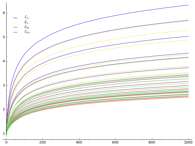
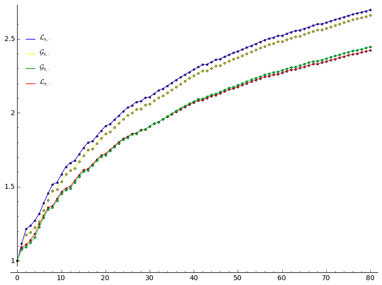
The idea that converges faster to 1 than as - or equivalently does not grow slower than - was motivated by Figure 3.1 which covers a much too small part for a reasonable confidence level. Another way to express the higher speed of convergence is the next claim which is equivalent to Claim 1.2.
Claim 4.6.
and if for some .
4.3 Oscillation Theorems
Clearly, everything works fine if RH is true. An indirect proof with osciallation theorems like [36, Corollaire 1], [44, Sec. 4], or [18, 4] will be proposed by showing that the minimal oscillations force above for sufficiently large. After all, Voros reported in [59, Ch. 11] that the amplitude of Keiper’s sequence grows exponentially, [22, 28, 6].
Definition 4.7.
Obviously RH is true if and only if the very critical strip coincides with the critical line.
Note 4.8.
-
1.
By definition and holf if and only if and are respectively false whereas means that is false, i.e. on some sequence of ’s is at least of order .
-
2.
D. E. Knuth preferred which is not quite the same, [23].
Assumption 4.9.
For the rest of the section let be in the very critical strip and the least exceptional number which fixes an index for the remaining section.
Corollary 4.11.
and are false, i.e. there are such that for every natural there are CA numbers for which and are true.
Definition 4.12.
Let for
The oscillation quotient is for .
Note 4.13.
Under Assumption 4.9 infinitely many changes of sign of were established by Robin referring to the contributions of Nicolas, Landau, and Grönwall.
Condition 4.14.
There are indices and with and .
Theorem 4.15.
There is no exceptional number under Condition 4.14.
Proof.
Lemma 4.16.
The oscillation quotient can be written as for
| (4.1) |
Proof.
Verify the factorisation by expanding the product on RHS. What remains follows from
∎
Definition 4.17.
Define three sets of points :
-
1.
Eligible points meet and for some ,
-
2.
the upper part is , and
-
3.
the big points are those in .
Claim 4.18.
The margin contains at least one eligible point.
Proof.
Definition 4.20.
Let
-
1.
for ,
-
2.
and , a context-sensitive notation.
Fact 4.21.
Lemma 4.22.
-
1.
if and .
-
2.
If and and for constant then
-
3.
.
Proof.
For from Lemma 4.16 it holds true that
-
1.
Both sides are equal to , and
-
2.
such that causes
- 3.
∎
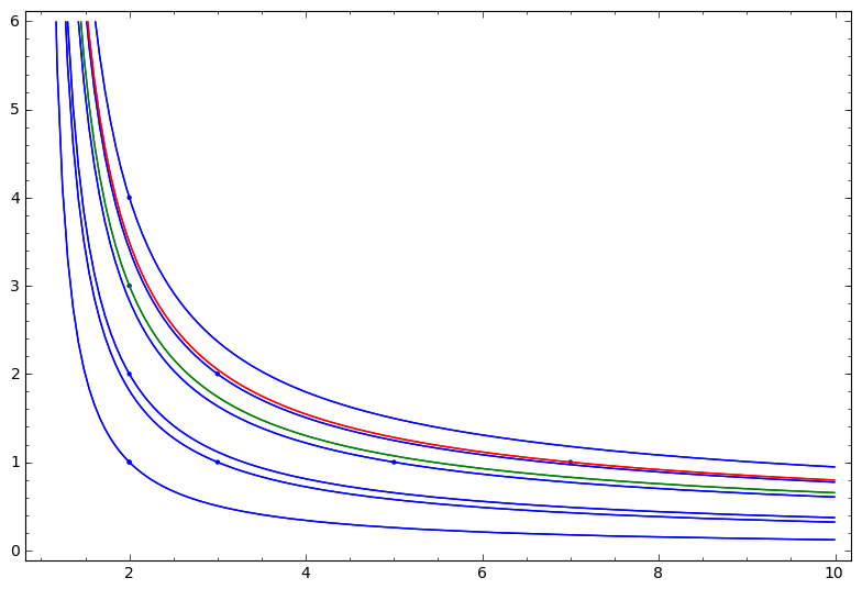
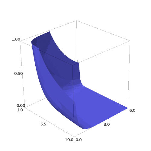
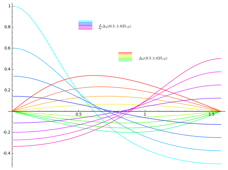
Figure 4.1: Contour Plot of and Cartesian Plots of , rf. Appendix
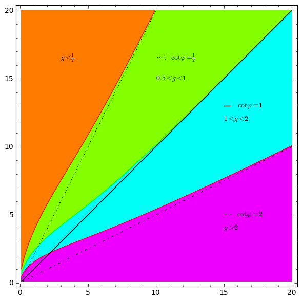
Multiplying by can be realised by adding to presuming and s.t. iff . With is decreasing in and has one change of sign. So as a function of has one minimal and one maximal turning point for and for , resp.
Corollary.
and if and then .
Proposition 4.23.
for and iff . Moreover iff such that for .
Proof.
holds if and only if which is true if and impossible unless . Likewise holds if and only if . A special case is for . ∎
Proposition 4.24.
Let be a sequence in with for and . Then as for the indices of a suitable subsequence. Moreover and for all natural .
Proof.
A sequence of indices with and can be chosen. in polar coordinates has the angle with for an arbitrarily fixed if is sufficiently large. has infinitely many members with since . Other members are not suitable.∎
Proposition 4.25.
If is an increasing sequence in with as then there is an index with .
Proof.
If was true for all then each would meet either or . Therefore follows from Proposition 4.23 for all where and . But this contradicts the assumption as .∎
Theorem 4.26.
[65]: for .
Proposition.
Polymath8:
The last theorem holds true with .
Corollary 4.27.
contains infinitely many pairs of consecutive primes.
Proof.
Figure 4.1a seems to show that the margin is essentially a bulge that only allows eligible points with small coordinates. But the so-called bulge depends on the choice of and disappears as approaches zero. The factor has a positive lower limit because of which the contour diverges away from the bisecting line. Because of the convergence the asymptote is given by .
Lemma 4.28.
as for every fixed real number .
Proof.
Put . Since as l’Hôspital’s rule implies
∎
Corollary 4.29.
If Assumption 2.9 is true then and as .
Proof.
Proposition 4.30.
Let be an increasing sequence in with . Then as for the indices of a suitable subsequence. Moreover and for all natural .
Proof.
A sequence of indices with can be chosen. holds for infinitely many members of because . In polar coordinates the points have the angle with for an arbitrarily fixed if is sufficiently large. Members with are not suitable.∎
Corollary 4.31.
contains eligible points.
Proof.
Proof.
A chain of reductions:
- 1.
- 2.
- 3.
- 4.
- 5.
∎
5 Final Remarks
Recently it has already been pointed out in [12, 10, 11] that RIE holds for all without requiring Assumption 2.9. Independently of this approach Conclusion 4.32 will have many consequences once Assumption 2.9 is established. A few of them are metioned.
- 1.
-
2.
The weakened version of the disproved Mertens conjecture.
- 3.
-
4.
There are infinitely many extremely abundant numbers, [35, Thm 2.4].
-
5.
The status of Cramér’s conjecture is still undecided but with Cramér’s work can be deduced for every gap.
-
6.
A recent result is Hypothesis P in [14] according to Proposition 40 in that paper.
- 7.
Approaches related to the present one are [35, 34] as well as [33, 2]. The former led to [34, Thm 1.7] and a sequence of increasing values of whose existence follows from Grönwall’s theorem with Robin’s Oscillation theorems. The latter pointed out that increasing values of on superabundant numbers are sufficient. CA numbers do not allow for the minimality condition. Exceptional numbers cause oscillations whereas the explicit formulas are more precise under RH. If oscillations prevent exceptional numbers RH could be said to be hoist by its own petard.
Acknowledgements
Unfortunately I never received the support I would have liked to thank for at this place for which there is a variety of reasons. However, I want to thank Dr. Thomas Severin for recommending to me to investigate RIE when I worked for the Allianz insurance company in 1997. Likewise I thank Alexander Rueff for his suggestion to study Ramanujan’s lost notebook during my first year at university. Thanks for helpful feedback from an anonymous referee. I appreciate many fruitful discussions with Sebastian Spang while I worked with him, again for the Allianz. I thank Keith Briggs for our conversation, too. Last not least I thank my cousin Benedict Scholl for an additional pair of eyes as it might have been difficult for him to provide the strictly non-mathematical review I asked for.
Appendix A Implementation
Results have already been mentioned above. Sage code follows below. My first version computed for two weeks last year on a MacBook Air until , i.e. was reached. A revised implementation did the job in a bit more than half an hour (without standby phases). There are two reasons for the difference:
-
1.
Pre-Computation of a list of primes,
-
2.
Consequent exploitation of the factorisation of CA numbers.
Because of assumption 2.9 it is only necessary to select the next prime in every loop, determine new primes that may follow next, and to compute the values of associated with the (in virtue of [40, §59] and [3, Thm 1] at most 2) additional new primes.
The following functions compute CA numbers as they were represented in section 3.2. Noe’s top-down form of primes triggering the next valuation is used to store . When has been computed the primes such that does not violate the basic SA condition are called candidates for , rf. [3, Theorem 2]. It is convenient that the candidates for are the primes that occur in the bottom-up form of .
TODO: in triggers and candidates store indices in sieve instead of elements of sieve, endow sieve with logs of primes, in addSievedPrimeToTriggers() avoid searching newprime in sieve.
Compute CA Numbers in top-down form, a potentially not so big CA number is to be given, e.g. counter = 4 and triggers = [5, 2], seems not to work with the known smaller CA numbers
-
sieve = prime_range(2, 50000000)
def getSubsequentCAnumber(counter, triggers, number, sieve):
k = 0
candidates = getBottomUpTriggers(triggers)
epsilons = map(lambda i: getCAparameter(candidates[i], i+1),
range(len(candidates)))
while k < number:
k = k + 1
vmax = selectNextTrigger(epsilons)
triggers = addSievedPrimeToTriggers(candidates[vmax], triggers,
candidates, epsilons, sieve)
return triggers
Convert CA Numbers to bottom-up form
-
def getBottomUpTriggers(triggers):
l = len(triggers); i = 0
result = []
while i<l:
p = triggers[i]; j = 1
if p!=0:
result.append(next_prime(p))
else:
p = triggers[i+j]
while p==0:
j=j+1
p = triggers[i+j]
result.append(next_prime(p))
result.extend([0 for dummy in range(j)])
j=j+1
i=i+j
result.append(2)
return result
Choose the next candidate
-
def selectNextTrigger(E):
emax = max(E)
vmax = [v for v in range(len(E)) if E[v] >= emax]
if len(vmax) > 1:
print "FOUR EXPONENTIALS DISPROVED!"
else:
return vmax[0]
Enter the next candidate in the list of triggering primes and update candidates and epsilons
-
def addSievedPrimeToTriggers(newprime, triggers, candidates, epsilons, sieve):
vmax = candidates.index(newprime)+1
npi = sieve.index(newprime)
i = vmax-1
l = len(triggers)
if i < l:
triggers[i] = newprime
if candidates[i+1] == 0:
candidates[i+1] = newprime
epsilons[i+1] = getCAparameter(newprime, vmax+1)
if triggers[i-1] == newprime:
triggers[i-1] = 0
candidates[i] = 0
epsilons[i] = 0
else:
candidates[i] = sieve[npi+1]
epsilons[i] = getCAparameter(candidates[i], vmax)
else:
triggers.append(newprime)
candidates.append(newprime)
vmax = vmax + 1
epsilons.append(getCAparameter(newprime, vmax))
if triggers[i-1] > 0:
triggers[i-1] = 0
candidates[i] = 0
epsilons[i] = 0
return triggers
Plotting and in Figure 4.1b.
-
DeltaPhi(x, phi) = arccot(x*cot(phi))-phi
P = sum([plot(DeltaPhi(i/8,phi), (phi, 0, pi/2),
rgbcolor = hue(((i+16)%20)/20)) for i in range(4, 13)])
P = P + sum([line([(0.8, 0.6-i/100), (0.9, 0.6-i/100)],
rgbcolor = hue(((i+16)%20)/20)) for i in range(4, 13)])
P = P + text(’$\\Delta\\varphi\\left(0.5:1.625,\\varphi\\right)$’,
(0.95, 0.5), color="black", horizontal_alignment=’left’)
P = P + sum([plot(DeltaPhi.diff(phi)(i/8,phi), (phi, 0, pi/2),
rgbcolor = hue(((i+6)%20)/20)) for i in range(4, 13)])
P = P + sum([line([(0.5, 0.9-i/100), (0.6, 0.9-i/100)],
rgbcolor = hue(((i+6)%20)/20)) for i in range(4, 13)])
(P+text(’$\\frac{\\partial}{\\partial\\varphi}
\\Delta\\varphi\\left(0.5:1.625,\\varphi\\right)$’,
(0.65, 0.8), color="black", horizontal_alignment=’left’)).show()
Compute
-
def getCAparameter(x, v):
if x == 0:
return 0
else:
if v == 0:
return log(1+1/x)/log(x)
else:
return log((1-x^(v+1))/(x-x^(v+1))) / log(x)
References
- [1] Milton Abramowitz and Irene Stegun. Handbook of Mathematical Functions: with Formulas, Graphs, and Mathematical Tables (Dover Books on Mathematics). Dover Publications, 1964.
- [2] Amir Akbary and Zachary Friggstad. Superabundant numbers and the riemann hypothesis. AMER MATH MON, 116(3):273–275, 2009.
- [3] Leonidas Alaoglu and Paul Erdős. On highly composite and similar numbers. Transactions of the American Mathematical Society, 56 (3):448–469, 1944.
- [4] R. J. Anderson and H. M. Stark. Oscillation theorems. In Marvin Isadore Knopp, editor, Analytic Number Theory: proceedings of a conference held at Temple University, Philadelphia, May 12-15, 1980, volume 899 of Lecture Notes in Mathematics, pages 79–106. University of Michigan, Springer, 1981.
- [5] Moree Nevans Banks, Hart. The nicolas and robin inequalities with sums of two squares. MONATSH MATH, 157(4):303–322, 2009.
- [6] Enrico Bombieri and Jeffrey C. Lagarias. Complements to li’s criterion for the riemann hypothesis. J. Number Theory, 77:274–287, 1999.
- [7] Keith Briggs. Abundant numbers and the riemann hypothesis. Experimental Mathematics, 15, 2006.
- [8] Nicolas Jean-Louis Caveney, Geoffrey and Jonathan Sondow. On sa, ca, and ga numbers. arXiv:1112.6010v1, 2011.
- [9] Nicolas Jean-Louis Caveney, Geoffrey and Jonathan Sondow. Robin’s theorem, primes, and a new elementary reformulation of the riemann hypothesis. arXiv:1110.5078v2, 2012.
- [10] Wang Juping Cheng, Yuanyou and Sergio Albeverio. Proof of the lindelöf hypothesis. arXiv:1010.3374, 2013.
- [11] Yuanyou Cheng. From the density and lindelöf hypotheses to prove the riemann hypothesis via a power sum method. arXiv:0810.2102, 2013.
- [12] Yuanyou Cheng and Sergio Albeverio. Proof of the density hypothesis. arXiv:0810.2103, 12 2008-2012.
- [13] Lichiardopol-N. Moree P. Choie, Y.-J. and P. Solé. On robin’s criterion for the riemann hypothesis. J. Théor. Nombres Bordeaux, 19(2):357–372, 2007.
- [14] Juan Arias de Reyna and Jan van de Lune. On the exact location of the non-trivial zeros of riemann’s zeta function. arXiv, 1305.3844:28, 2013.
- [15] Pierre Dusart. The th prime is greater than for . MATHEMATICS OF COMPUTATION, 68(225):411–415, 1999.
- [16] Paul Erdős and Jean-Louis Nicolas. Répartition des nombres superabondants. Bull. Soc. Math. France, 103:65–90, 1975.
- [17] Thomas H. Grönwall. Some asymptotic expressions in the theory of numbers. Trans. Amer. Math. Soc., 14:113 – 122, 1913.
- [18] Emil Grosswald. Oscillation theorems of arithmetical functions. Trans. Amer. Math. Soc., 126:1–28, 1967.
- [19] Geoffrey H. Hardy and John E. Littlewood. Some problems of diophantine approximation. Acta Mathematica, 37:225, 1914.
- [20] Geoffrey H. Hardy and Edward M. Wright. An Introduction to the Theory of Numbers. Oxford University Press, Oxford, England, 5 edition, 1979.
- [21] Alan Jeffrey. Handbook of Mathematical Formulas and Integrals, Third Edition. Academic Press, 2003.
- [22] J. B. Keiper. Power series expansions of riemann’s function. Math. Comput., 58:765–773, 1992.
- [23] Donald E. Knuth. Big omicron and big omega and big theta. In SIGACT News, pages 18–24, Apr.-June 1976.
- [24] Donald E. Knuth. The Art Of Computer Programming - Fundamental Algorithms. Addison-Wesley, 1997.
- [25] Edmund Landau. Handbuch der Lehre von der Verteilung der Primzahlen. Teubner, Leipzig, 1909.
- [26] Edmund Landau. Über die anzahl der gitterpunkte in gewissen bereichen. Nachrichten von der Gesellschaft der Wissenschaften zu Göttingen, Mathematisch-Physikalische Klasse, 1924:137–150, 1924.
- [27] Serge Lang. Introduction to Transcendental Numbers. Number 4178 in Addison-Wesley series in mathematics. Addison-Wesley, Reading, Mass., 1966.
- [28] Xian-Jin Li. The positivity of a sequence of numbers and the riemann hypothesis. Journal of Number Theory, 65(2):325–333, 1997.
- [29] Peter Lindqvist and Jaak Peetre. On the remainder in a series of mertens. Expositiones Mathematicae, 15:467–478, 1997.
- [30] John E. Littlewood. Sur la distribution des nombres premiers. Comptes rendus hebdomadaires des séances de l’Académie des sciences, 1914:1869–1872, 158.
- [31] Jean-Pierre Massias and Guy Robin. Bornes effectives pour certaines fonctions concernant les nombres premiers. J. Théor. Nombres Bordeaux, 8(1):215–242, 1996.
- [32] Franz Mertens. Ein beitrag zur analytischen zahlentheorie. Journal für die reine und angewandte Mathematik, 78:46–62, 1874.
- [33] Aleksandr Morkotun. On the increase of grönwall function value at the multiplication of its argument by a prime. arXiv, 1307.0083, July 2013.
- [34] Sadegh Nazardonyavi and Semyon Yakubovich. Delicacy of the riemann hypothesis and certain subsequences of superabundant numbers. arXiv, 1306.3434, June 2013.
- [35] Sadegh Nazardonyavi and Semyon Yakubovich. Superabundant numbers, their subsequences and the riemann hypothesis. arXiv, 1211.2147v3, February 2013.
- [36] Jean-Louis Nicolas. Petites valeurs de la fonction d’euler. Journal of Number Theory, 17(3):375 – 388, 1983.
- [37] T. D. Noe. First 500 superabundant numbers. 2005.
- [38] T. D. Noe. First 1000000 superabundant numbers. 2009.
- [39] Srinivasa Ramanujan. Highly composite numbers. Proc. London Math. Soc., 14:347–407, 1915.
- [40] Srinivasa Ramanujan. Highly composite numbers. The Ramanujan Journal, 1:119–153, 1997.
- [41] Paulo Ribenboim. The little book of big primes. Springer Verlag, 1991.
- [42] Hans Riesel. Prime Numbers and Computer Methods for Factorization. Modern Birkhäuser Classics. Springer, 2 edition, November 2011.
- [43] Marcel Riesz. Sur l’hypothèse de riemann. Acta Arith., 40:185 – 190, 1916.
- [44] Guy Robin. Sur l’ordre maximum de la fonction somme des diviseurs. Séminaire de théorie des nombres, Paris - Birkhauser, pages 233 – 244, 1981-82, 1983.
- [45] Guy Robin. Estimation de la fonction de tchebychef sur le k-ième nombre premier et grandes valeurs de la fonction nombre de diviseurs premiers de . Acta Arithmetica, 42(4):367 – 389, 1983.
- [46] Guy Robin. Grandes valeurs de la fonction somme des diviseurs et hypothèse de riemann. Journal de Mathématiques Pures et Appliquées. Neuvième Série, 63 (2):187 – 213, 1984.
- [47] Rosser and Schoenfeld. Sharper bounds for the chebyshev functions and (part i). Math. Comput., 29(129):243–269, JANUARY 1975.
- [48] Barkley Rosser. The -th prime is greater than . Proceedings of the London Mathematical Society, 2(1):21–44, 1939.
- [49] I. B. Rosser and L. Schoenfeld. Approximate formulas for some functions of prime numbers. Illinois J. Math., 6:64–94, 1962.
- [50] Lowell Schoenfeld. Sharper bounds for the chebyshev functions and , part ii. Math. Comput., 30(134):337–360, Aptil 1976.
- [51] Neil J. A. Sloane. The on-line encyclopedia of integer sequences® (oeis®).
- [52] Michel Solé, Patrick; Planat. Extreme values of the dedekind function. arXiv, 1011.1825, January 2011.
- [53] Michel Solé, Patrick; Planat. Robin inequality for 7-free integers. Electronic Journal of Combinatorial Number Theory, 11(11), December 2011.
- [54] Andreas Speiser. Geometrisches zur riemannschen zetafunktion. Math. Ann., 110:514 – 521, 1934. Mathematische Annalen.
- [55] The Sage Development Team. Sage reference. 5.2, 2005–2011.
- [56] Ambler Thompson and Barry N. Taylor. Guide for the use of the international system of units (si), March 2008.
- [57] Priscilla Throop. Isidore of Seville’s Etymologies: Complete English Translation, volume I of Isidore of Seville’s Etymologies: The Complete English Translation of Isidori Hispalensis Episcopi Etymologiarum Sive Originum Libri XX. Lulu.Com, paperback edition, 2006.
- [58] Mark B. Villarino. Mertens’ proof of mertens’ theorem. 2005.
- [59] André Voros. Zeta Functions over Zeros of Zeta Functions, volume 8 of Lecture Notes of the Unione Matematica Italiana. Springer, 2010. ISBN 978-3-642-05202-6.
- [60] Michel Waldschmidt. Nombres transcendants. Lecture notes in mathematics. Springer, Berlin, 1974.
- [61] Michel Waldschmidt. Diophantine approximation on linear algebraic groups. Die Grundlehren der mathematischen Wissenschaften in Einzeldarstellungen. Springer, Berlin, 2000.
- [62] Jimmy Wales and Larry Sanger. Wikipedia, the free encyclopedia.
- [63] André Weil. Sur les ’formules explicites’ de la théorie des nombres premiers. Comm. Lund, vol. dédié a Marcel Riesz:252–265, 1952. Collected Papers II.
- [64] Eric W. Weisstein. CRC Concise Encyclopedia of Mathematics. CRC Press, 1999.
- [65] Yitang Zhang. Bounded gaps between primes. Annals of Mathematics, 2013. to appear.