11email: Morgan.Deal@astro.up.pt, Carlos.Martins@astro.up.pt 22institutetext: Instituto de Astrofísica e Ciências do Espaço, CAUP, Rua das Estrelas, 4150-762 Porto, Portugal
Primordial nucleosynthesis with varying fundamental constants
The success of primordial nucleosynthesis has been limited by the long-standing Lithium problem. We use a self-consistent perturbative analysis of the effects of relevant theoretical parameters on primordial nucleosynthesis, including variations of nature’s fundamental constants, to explore the problem and its possible solutions, in the context of the latest observations and theoretical modeling. We quantify the amount of depletion needed to solve the Lithium problem, and show that transport processes of chemical elements in stars are able to account for it. Specifically, the combination of atomic diffusion, rotation and penetrative convection allows us to reproduce the lithium surface abundances of Population II stars, starting from the primordial Lithium abundance. We also show that even with this depletion factor there is a preference for a value of the fine-structure constant at this epoch that is larger than the current laboratory one by a few parts per million of relative variation, at the two to three standard deviations level of statistical significance. This preference is driven by the recently noticed discrepancy between the best-fit values for the baryon-to-photon ratio (or equivalently the Deuterium abundance) inferred from cosmic microwave background and primordial nucleosynthesis analyses, and is largely insensitive to the Helium-4 abundance. We thus conclude that the Lithium problem most likely has an astrophysical solution, while the Deuterium discrepancy provides a possible hint of new physics.
Key Words.:
Nuclear reactions, nucleosynthesis, abundances – (Cosmology:) primordial nucleosynthesis – Stars: abundances – Stars: evolution – Cosmology: theory – Methods: statistical1 Introduction
Big Bang Nucleosynthesis (henceforth BBN) is a cornerstone of the standard particle cosmology paradigm, and a sensitive probe of physics beyond the standard model (Steigman, 2007; Iocco et al., 2009; Pitrou et al., 2018). Nevertheless, its success is limited by the well-known Lithium problem, wherein the theoretically expected abundance of Lithium-7 (given our present knowledge of astrophysics, nuclear and particle physics) exceeds the observed one by a factor of about 3.5 (Zyla et al., 2020). Although there have been many attempts to solve the problem, there is no clear known solution. Further discussion of these solutions can be found in Fields (2011), Mathews et al. (2020) and the BBN section of the latest Particle Data Group (henceforth PDG) review by Zyla et al. (2020).
Recent progress in experimental measurements of the required nuclear cross-sections has all but excluded the possibility of nuclear physics systematics (Iliadis & Coc, 2020; Mossa et al., 2020). On the astrophysics side, some degree of lithium depletion can occur in stars due to the mixing of the outer layers with the hotter interior (Sbordone et al., 2010), and some authors have suggested that a depletion by factor as large as 1.8 may have occurred (Ryan et al., 2000; Korn et al., 2006). It has been argued that this scenario might be difficult to reconcile with the existence of extremely iron-poor dwarf stars with lithium abundances very close to the Spite plateau (Aguado et al., 2019), but there is no consensus on this point. Finally, the Lithium problem could also point to new physics beyond the standard model; one such possibility is the variation of nature’s fundamental constants, which is unavoidable in many extensions of the standard particle physics and cosmological models (Damour et al., 2002)—a recent review of the topic is Martins (2017). This possibility has been recently revisited in Clara & Martins (2020) and Martins (2021) (henceforth Paper 1 and Paper 2, respectively), who show that there is a preference for a value of the fine-structure constant, , at the BBN epoch that is larger than the current laboratory one by a few parts per million of relative variation, even when allowing for possible changes to the most relevant cosmological parameters impacting BBN: the neutron lifetime, the number of neutrino species, the and baryon-to-photon ratio.
Stars are formed with an initial chemical composition representative of their birth environment. During their evolution, this chemical composition is modified by several processes, namely nuclear reactions and transport processes. Nuclear reactions affect the abundance profiles of some elements in the central region of stars, increasing or decreasing their abundances. Transport processes of chemical elements modify the elements distribution in the whole star. There are macroscopic transport processes as, for example, convection, which efficiently transports chemical elements and leads to an homogenized chemical composition in the convective zone. Other macroscopic transport processes are less efficient and reduce the potential internal gradient of chemical composition while transporting them deeper in stars (i.e. transport induced by the rotation: e.g. Palacios et al. 2003, and references therein; Talon 2008, and references therein; Maeder 2009, and references therein, thermohaline convection: e.g. Vauclair 2004, and references therein; Denissenkov 2010, and references therein; Brown et al. 2013, and references therein; Deal et al. 2016, and references therein). These macroscopic transport processes are in competition with microscopic transport processes, namely atomic diffusion (see Michaud et al., 2015, for a detailed description). This comes from physics first principles and is induced by the internal gradients of pressure, temperature and composition. It is efficient in radiative zones and leads to a selective transport of chemical elements, mainly driven by the competition between the gravity and radiative accelerations. Gravity moves elements towards the center of stars while radiative accelerations, a mechanism for transfer of momentum between photons and ions, move some elements toward the surface of stars (depending on their ionisation states and abundances). As a consequence, the surface abundance of elements are either larger or smaller than the initial ones. Considering all the potential processes affecting the chemical elements distribution in stars, it is expected that observed surface abundances are often different from the initial ones, especially on the main sequence where the surface convective zones are not too deep to allow surface abundance variations.
Light elements (such as lithium and beryllium) are especially impacted by transport processes during the evolution of stars. Atomic diffusion leads to a depletion of these elements from the surface (radiative accelerations are most of the time negligible for these elements). Moreover, these elements are destroyed by nuclear reactions at rather low temperatures (about and million K for lithium and beryllium, respectively), not very deep inside stars. When macroscopic transport processes are efficient enough and affect deep regions, lithium is then transported in regions where the temperature is large enough to be destroyed by nuclear reactions. The combination of both atomic diffusion and macroscopic transport processes is expected to lead to a discernible depletion of lithium from the surface, hence to lithium-7 surface abundances smaller than the initial one (e.g. Vauclair, 1988; Charbonnel et al., 1994; Korn et al., 2006, 2007; Gruyters et al., 2013, 2016; Dumont et al., 2020).
Population II stars are not an exception and undergo the same kind of depletion thanks to the same processes (e.g. Michaud et al., 1984; Richard et al., 2005). This is the reason why the lithium-7 surface abundances observed in population II stars (known as the Spite plateau, Spite & Spite 1982) are most likely not the initial ones, hence the discrepancy with a larger cosmological lithium-7 abundance (from BBN). It is interesting to note that a lot of stars are found to have a lithium abundance smaller than the lithium plateau (Bonifacio et al., 2007; Cayrel et al., 2008; Sbordone et al., 2010), which can also be explained by stellar models, for example, in the case of carbon enhanced metal poor stars with excess in s process elements (CEMP-s stars) (e.g. Stancliffe, 2009; Deal et al., 2021).
Here we draw on the self-consistent perturbative analysis formalism introduced in Paper 1 and extended in Paper 2 to revisit the role of stellar depletion in the Lithium problem, while simultaneously allowing for time variation of nature’s fundamental constants, in a broad class of Grand Unified theory (GUT) scenarios where all the gauge and Yukawa couplings are allowed to vary. It will be seen that the impacts of the two mechanisms can be separately constrained. We will start by assuming that the there is a depletion factor relating the cosmological and astrophysical lithium-7 abundances
| (1) |
Throughout our statistical analyses is allowed to span the entire range, under the assumption of a uniform prior. Clearly this is a purely phenomenological parameter, and given any pair or cosmological and astrophysical lithium abundances, for which the former is larger than the latter, there will always be a choice of that makes the two compatible. In this sense, the observed lithium-7 abundance simply provides a measurement of . However, the hypothesis underlying this assumption is that there exist stellar physics mechanisms and/or physical transport processes occurring in stars that can account for the the relevant value of . Thus our purpose in introducing Eq. (1) is twofold. Firstly, it will allow us to quantify the impact of astrophysical depletion in models which also allow for new physics mechanisms (specifically, in the present work, through varying fundamental constants), thereby comparing the possible roles of the two. Secondly, it provides a convenient way to assess the extent to which stellar physics mechanisms could lead to depletion.
Following the approach of Paper 1 and Paper 2, we have done our statistical likelihood analyses using three different combinations of the four abundances, as follows
-
•
The baseline case uses the abundances of helium-4, deuterium and lithium-7, which are the three available cosmological abundances. This will providing the reference values for the best-fit BBN values for .
-
•
The extended case adds the helium-3 abundance to the former three; this separation stems from the fact that its observed abundance is a local rather than a cosmological one. In any case, as was pointed out in Paper 1 and Paper 2, this has a negligibly small impact on the derived constraints.
-
•
The null case, which uses the helium-4, deuterium and helium-3 abundances but does not use lithium-7. The motivation for this case is that it provides a useful null test of the BBN sensitivity to the value of the fine-structure constant. In other words, if all the relevant physics is the standard one, it is expected that the standard value of is recovered in this case to some degree of sensitivity that is useful to quantify and compare to other probes, It also provides an indication of the BBN constraints on on the assumption that the Lithium problem has an astrophysical solution.
For convenience, we will use the Baseline, Extended and Null terms to denote each of the three combinations when presenting the results in figures in the early part of the work. (This facilitates comparisons with the results in Paper 1 and Paper 2.) In the later part, and when summarizing results in the text and tables throughout the work, we will concentrate on the Baseline case, with Null case results provided for comparison when relevant.
The plan of the rest of this work is as follows. We start in Sect. 2 by phenomenologically quantifying the preferred depletion factor assuming that the three key cosmological parameters—the neutron lifetime, number of neutrinos and baryon-to-photon ratio—are allowed to vary, but constrained by priors external to BBN. In Sect. 3, we report on the analogous study for GUT scenarios where all the gauge and Yukawa couplings are allowed to vary, confirming the previously reported preference for a larger value of at the BBN epoch. In this case the baryon-to-photon ratio and number of neutrinos are assumed to be fixed at their standard values, while the neutron lifetime is unavoidably affected. Together, these two sections confirm a discrepancy in the values of the baryon-to-photon ratio—or equivalently the primordial Deuterium abundance—preferred by BBN and cosmic microwave background (CMB) plus baryon acoustic oscillation (BAO) data, which has been recently reported (Pitrou et al., 2021; Yeh et al., 2021). In Sect. 4 we address the Lithium problem, showing that the combination of atomic diffusion, rotation and penetrative convection can bridge the gap between the cosmological abundance and the surface abundances measured in Population II stars. In Sect. 5 we address the Deuterium discrepancy, showing that it (and not the Lithium problem) is driving the aforementioned preference for a larger value of and further quantifying the model dependence of this preference. Finally, we offer some conclusions in Sect. 6.
2 Depletion and cosmological parameters
Generically, the sensitivity of the primordial BBN abundances to the various relevant model parameters can be described as
| (2) |
where are the sensitivity coefficients. The perturbation is always done with respect to the predicted abundance values in some baseline theoretical model, which in our case is the one recently presented in Pitrou et al. (2021). These predicted abundances are listed in Table 1 for convenience, together with the observed abundances as recommended by the BBN review in Zyla et al. (2020). The two are compared using standard statistical likelihood methods, and theoretical and observational uncertainties being added in quadrature. We note that our fiducial model differs from the one used in Paper 1 and Paper 2, which was based on the earlier work of Pitrou et al. (2018). Therefore our present results can be approximately (but not exactly) compared with those of the earlier papers.
| Abundance | Theoretical | Observed |
|---|---|---|
In this section we consider the effect of the values of the neutron lifetime , the number of neutrino species , and the baryon-to-photon ratio (where, for convenience, we have defined ) on the BBN abundances. The fiducial values of these parameters (which will be used as statistical Gaussian priors in the analysis) are, respectively
| (3) |
for the neutron lifetime (Zyla et al., 2020) (see also Rajan & Desai (2020) for a recent discussion of experimental measurements of this lifetime),
| (4) |
for the number of neutrino species, which comes from the LEP measurement (Zyla et al., 2020), and
| (5) |
from the combination of recent CMB (Planck 2018) and BAO data (Aghanim et al., 2020). For reference, the latter corresponds to the physical baryon density
| (6) |
| D | 3He | 4He | 7Li | |
|---|---|---|---|---|
| +0.442 | +0.141 | +0.732 | +0.438 | |
| +0.409 | +0.136 | +0.164 | -0.277 | |
| -1.65 | -0.567 | +0.039 | +2.08 |
With these assumptions our perturbative analysis for the BBN abundances has the specific form
| (7) |
where , and are the sensitivity coefficients listed in Table 2 and previously discussed in Paper 2 and references therein. Note that Deuterium is far more sensitive to the baryon fraction than to the neutron lifetime or the number of neutrinos, while the opposite occurs for Helium-4. Additionally, we will make the assumption that the cosmological and astrophysical lithium-7 abundances are related through Eq. (1), so the depletion factor becomes a fourth model parameter, together with the relative variations of the three cosmological parameters.
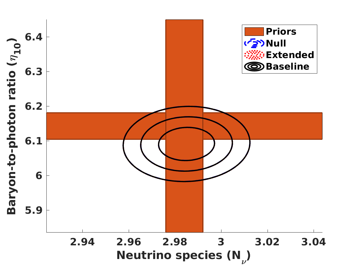
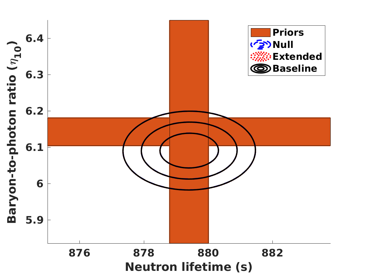
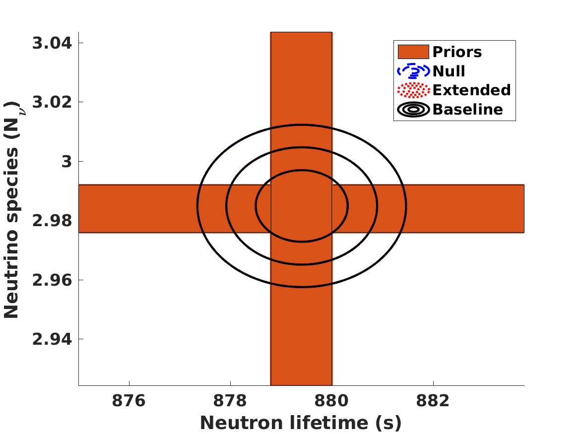
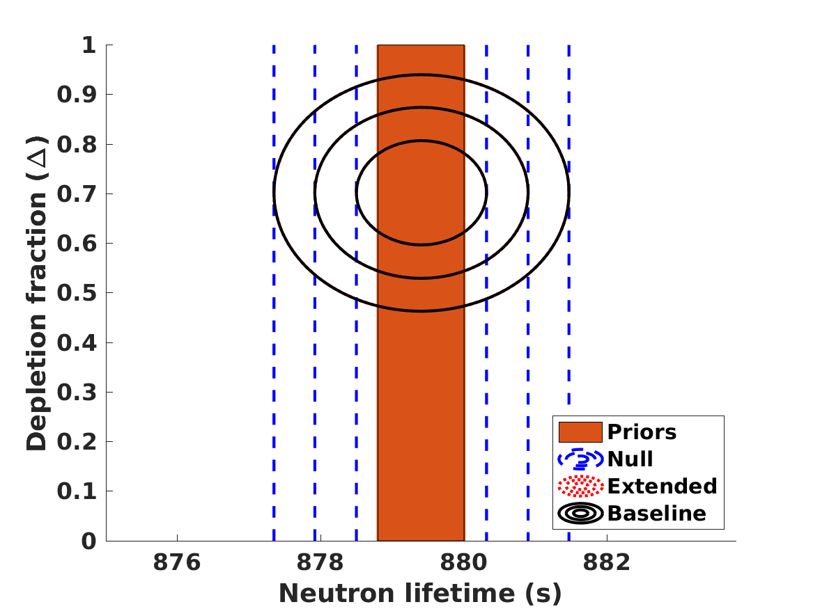
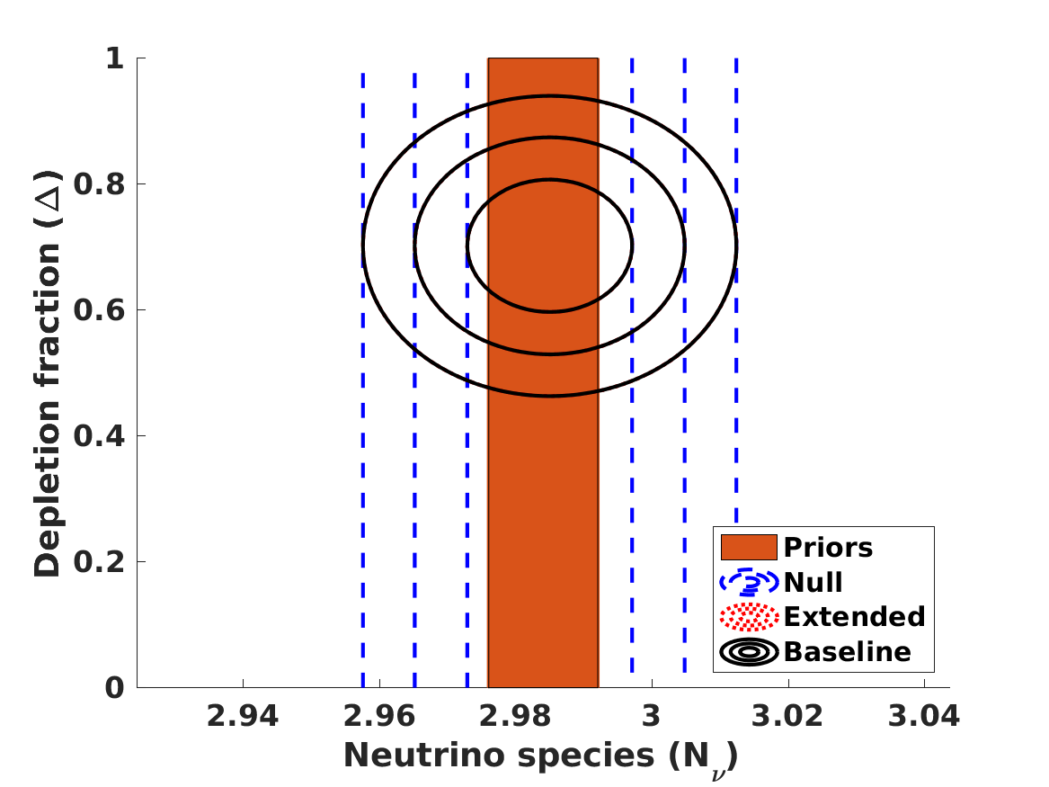
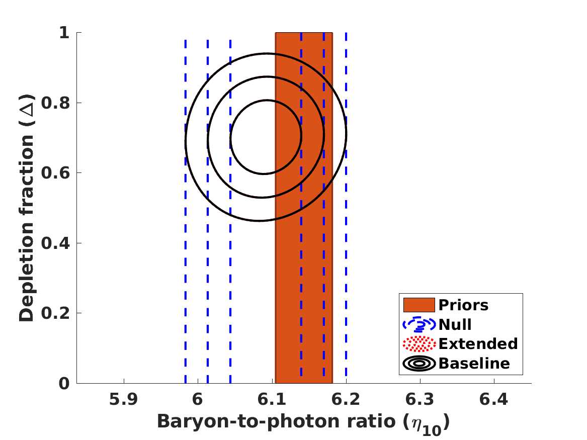
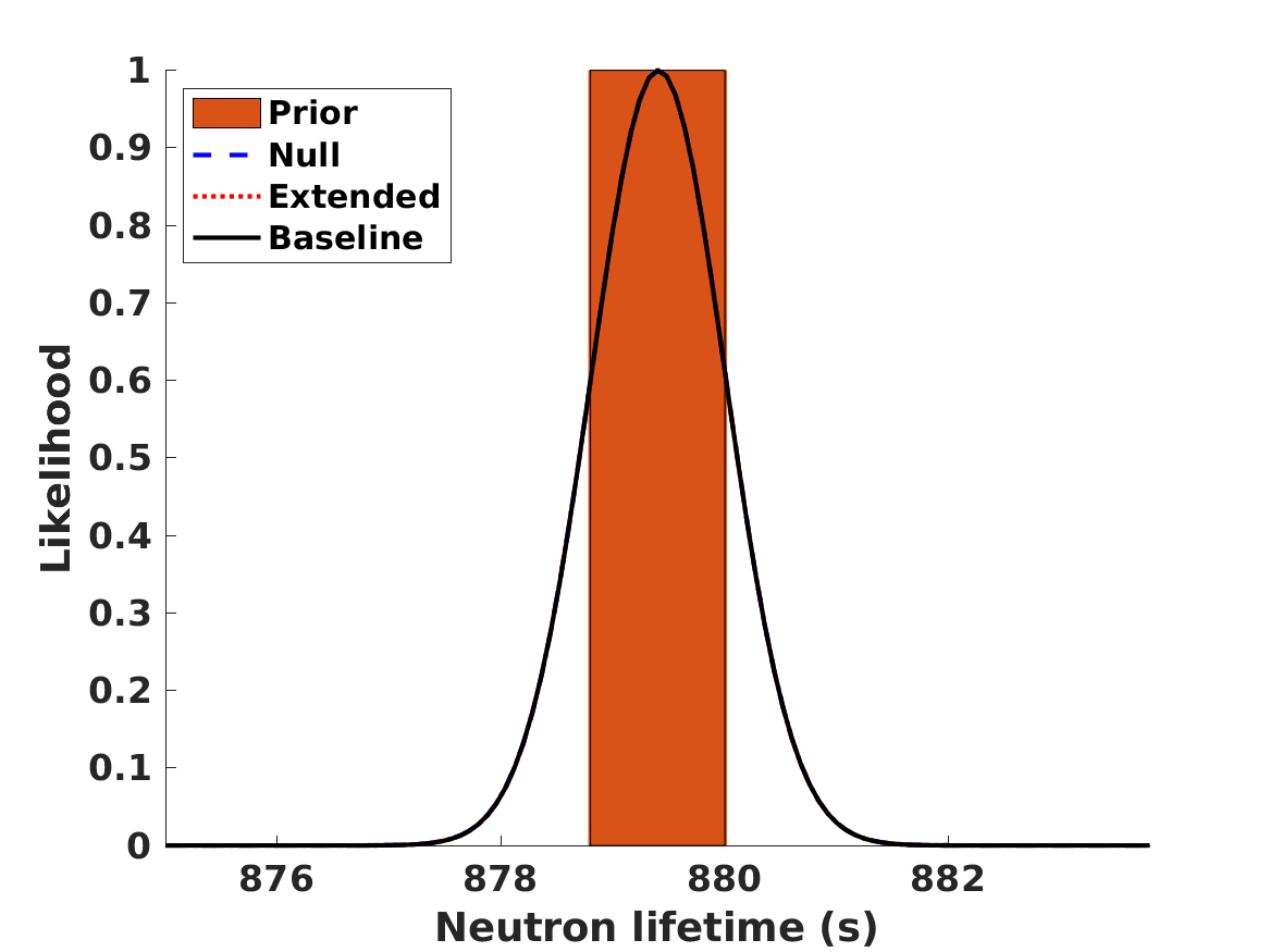
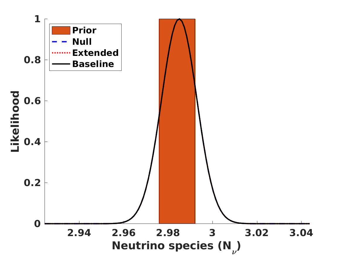
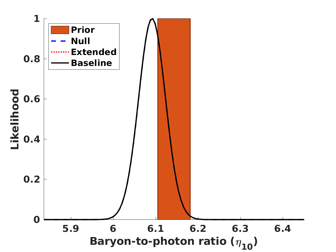
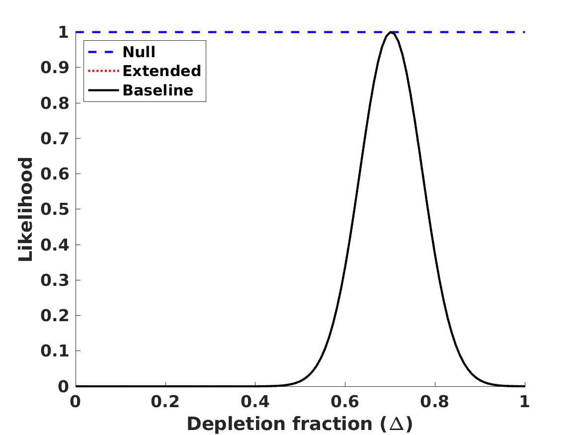
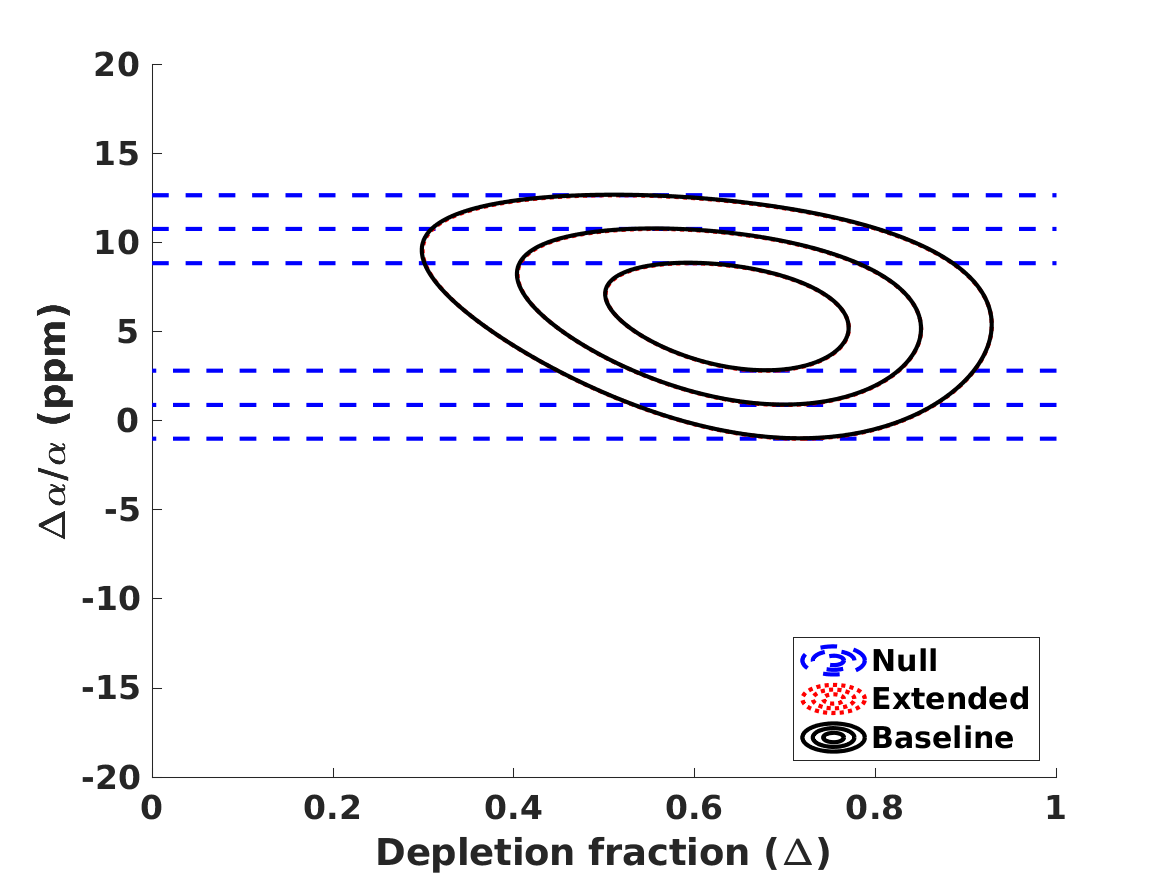
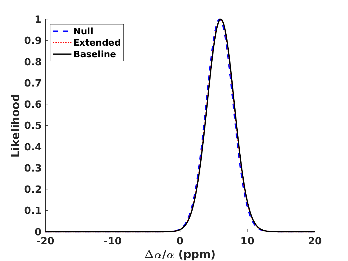
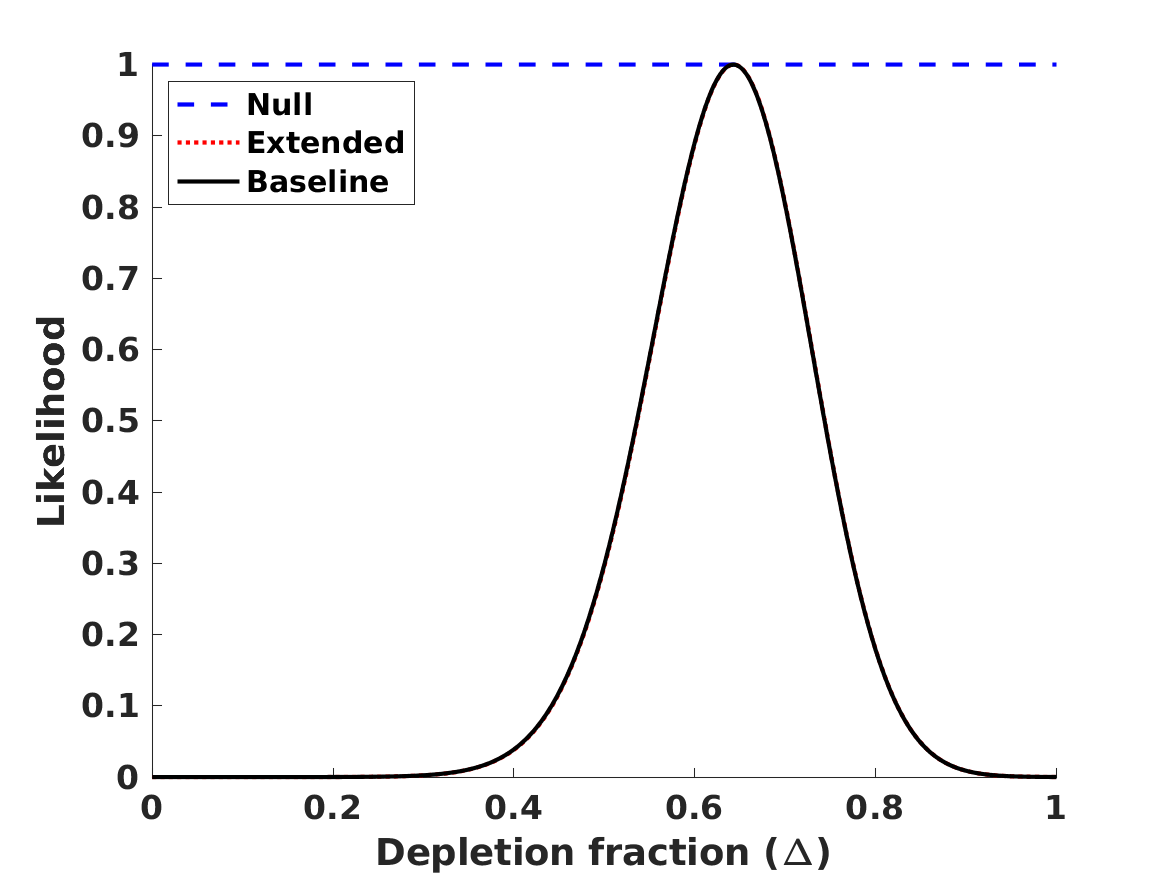
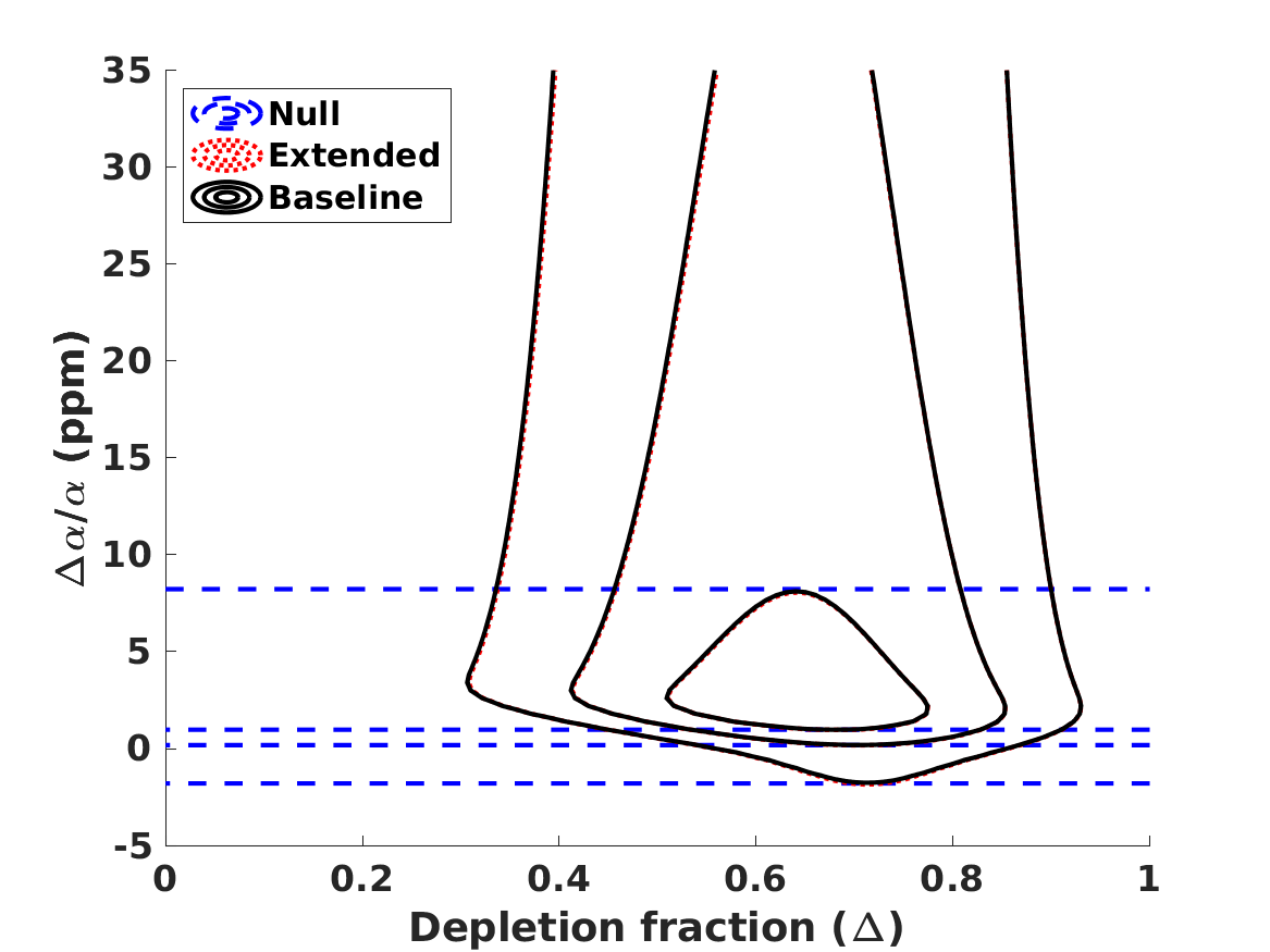
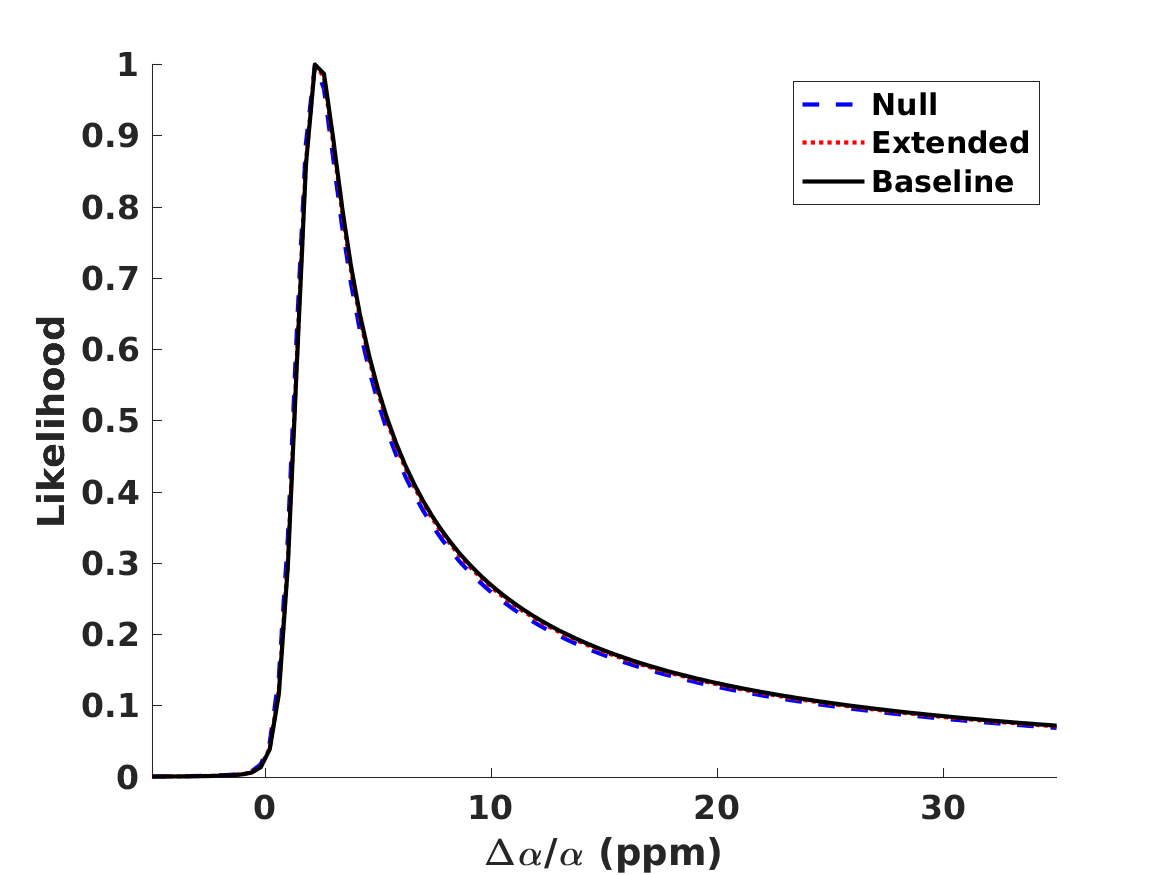
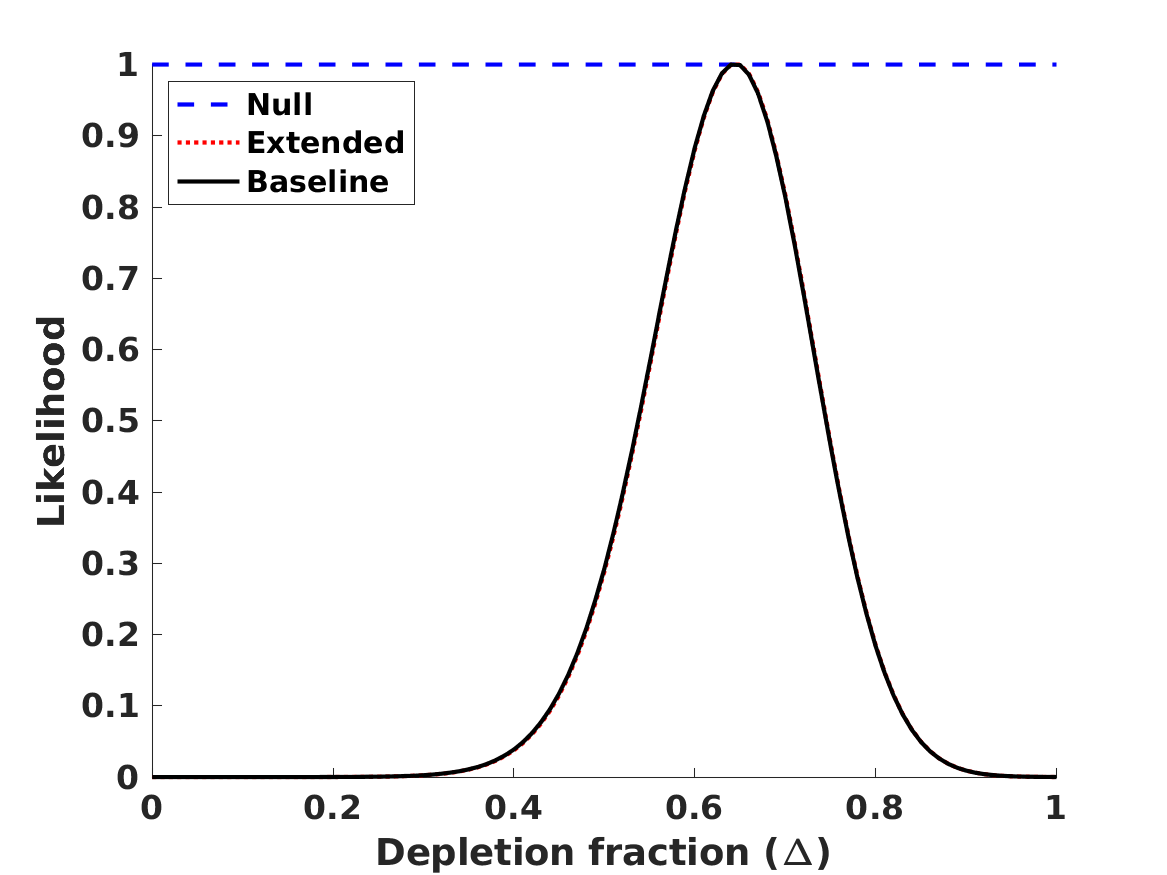
The results of the analysis are depicted in Figure 1. The best-fit values of our free parameters (with their one standard deviation uncertainties) in the Baseline case are
| (8) | |||||
| (9) | |||||
| (10) | |||||
| (11) |
in the Null case the first three of these are the same, while is obviously not constrained. (On the other hand, if one assumes that , and are fixed at their fiducial values rather than allowed to vary and marginalized, one finds .) These lead to the following best fit theoretical abundances
| (12) | |||||
| (13) | |||||
| (14) | |||||
| (15) | |||||
| (16) |
for lithium-7 we separately list the cosmological (primordial) abundance, and the corresponding astrophysical one, corrected by the preferred seventy percent depletion. We confirm the result, already mentioned by Pitrou et al. (2021), that with the latest nuclear physics cross sections and observed abundances the BBN observations prefer a slightly lower than the one measured by the combination of CMB and BAO observations. Alternatively, this can be phrased as as discrepancy in the Deuterium abundance. On the other hand, different reaction rates are used in Yeh et al. (2021) and in Pisanti et al. (2021), which find no such discrepancy. In any case, as illustrated in Figure 1, the discrepancy is only slightly larger than one standard deviation, so its statistical significance is limited. We revisit this point later in this work.
3 Depletion and Varying fundamental constants
The approach introduced Paper 1 and Paper 2 to study BBN with varying fundamental constants is also a perturbative one. It builds upon earlier work by Muller et al. (2004) and Flambaum & Wiringa (2007) and subsequent developments by Coc et al. (2007) and Dent et al. (2007), to generically write the relative variations of other couplings as the product of some constant particle physics coefficients and the relative variation of the fine-structure constant. With some reasonable simplifying assumptions, which stem from the work of Campbell & Olive (1995), only two such dimensionless coefficients are needed, one pertaining to electroweak physics (denoted ) and the other to strong interactions (denoted ). This enables a phenomenological description of a broad range of GUT scenarios. We refer the reader to Paper 1 and Paper 2 for a more detailed description of this formalism. In what follows, astrophysical constraints on are expressed in terms of a relative variation with respect to the local laboratory value,
| (18) |
where is the local laboratory value.
Under these assumptions, the sensitivity of the primordial BBN abundances to the values of the fundamental constants will therefore be expressed as a function of the phenomenological particle physics parameters and and the relative variation of , in other words
| (19) |
the corresponding sensitivity coefficients are listed in Table 3. Note that the baryon-to-photon ratio and number of neutrinos are assumed to be fixed at their standard values. On the other hand the neutron lifetime will be affected by the variation, according to
| (20) |
but this effect has been included in the computation of these sensitivity coefficients, so the neutron lifetime does not appear as an explicit parameter. We refer the reader to Paper 2 for a more detailed discussion.
| D | 3He | 4He | 7Li | |
|---|---|---|---|---|
| +42.0 | +1.27 | -4.6 | -166.6 | |
| +39.2 | +0.72 | -5.0 | -151.6 | |
| +36.6 | -89.5 | +14.6 | -200.9 |
The phenomenological parameters and can in principle be taken as free parameters, to be experimentally or observationally constrained. Our current knowledge of particle physics and unification scenarios suggests that their absolute values can be anything from order unity to several hundreds, with allowed to be positive or negative (though with the former case being the more likely one), while is expected to be non-negative.
The analysis of Paper 1 and Paper 2 has identified three models that can provide a solution to the Lithium problem (at least in the sense of making all theoretical and observed abundances agree to within three standard deviations or less) for the best-fit values of listed in Table 4. Note that the fiducial model used in these papers is not the same as the one used in the present work, and that the full parameter space was different in the two papers.
| Scenarios | Unification | Dilaton | Clocks |
|---|---|---|---|
| Paper 1 (Baseline) | |||
| Paper 1 (Null) | |||
| Paper 2 (Baseline) | |||
| Paper 2 (Null) |
The first of these is a ‘typical’ unification scenario, for which one has (Coc et al., 2007; Langacker et al., 2002)
| (21) |
we refer to this as the Unification model. The second is the dilaton-type model discussed by Nakashima et al. (2010), for which
| (22) |
we refer to this as the Dilaton model. Finally the Clocks model denotes the general case where the parameters and are allowed to vary and are then marginalised, in this case with uniform priors in the range , , together with an additional prior coming from local experiments with atomic clocks (Ferreira et al., 2012)
| (23) |
This is therefore a more phenomenological model than the previous two (and has a larger number of free parameters than them), but serves the purpose of illustrating the range of behaviours that might be found in GUT models—although we should mention that, unsurprisingly, the results in this case will also depend on the choice of priors for and . This last point has been discussed in Paper 1.
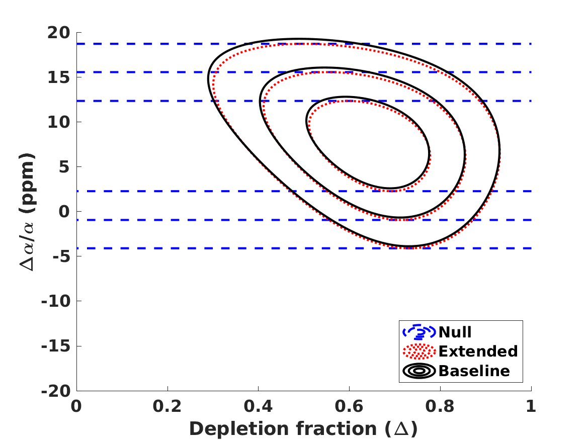
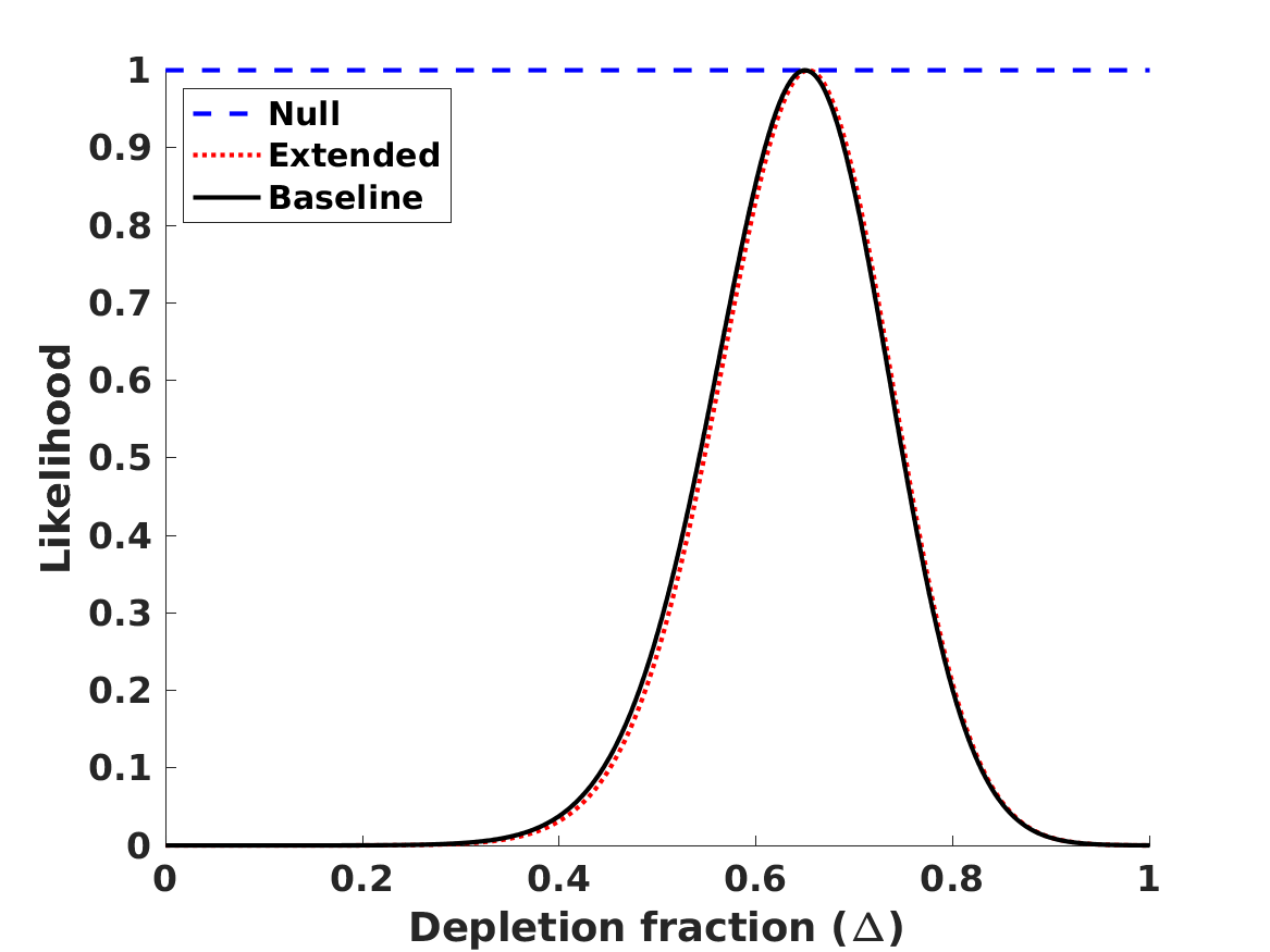
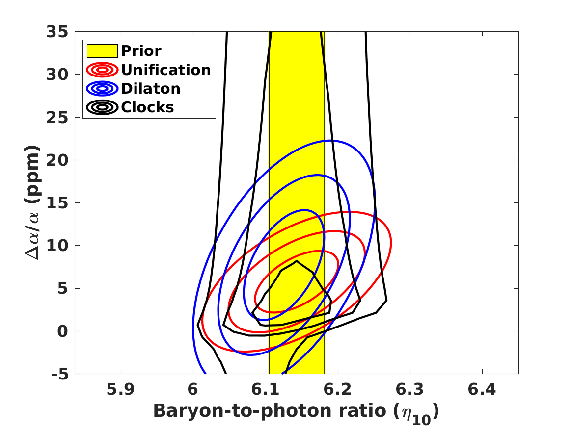
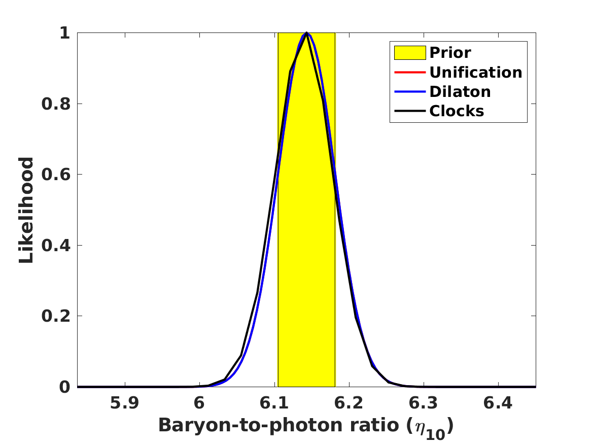
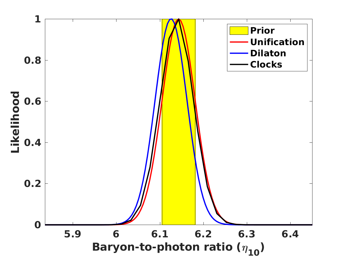
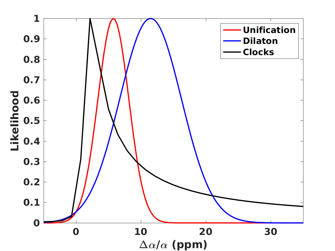
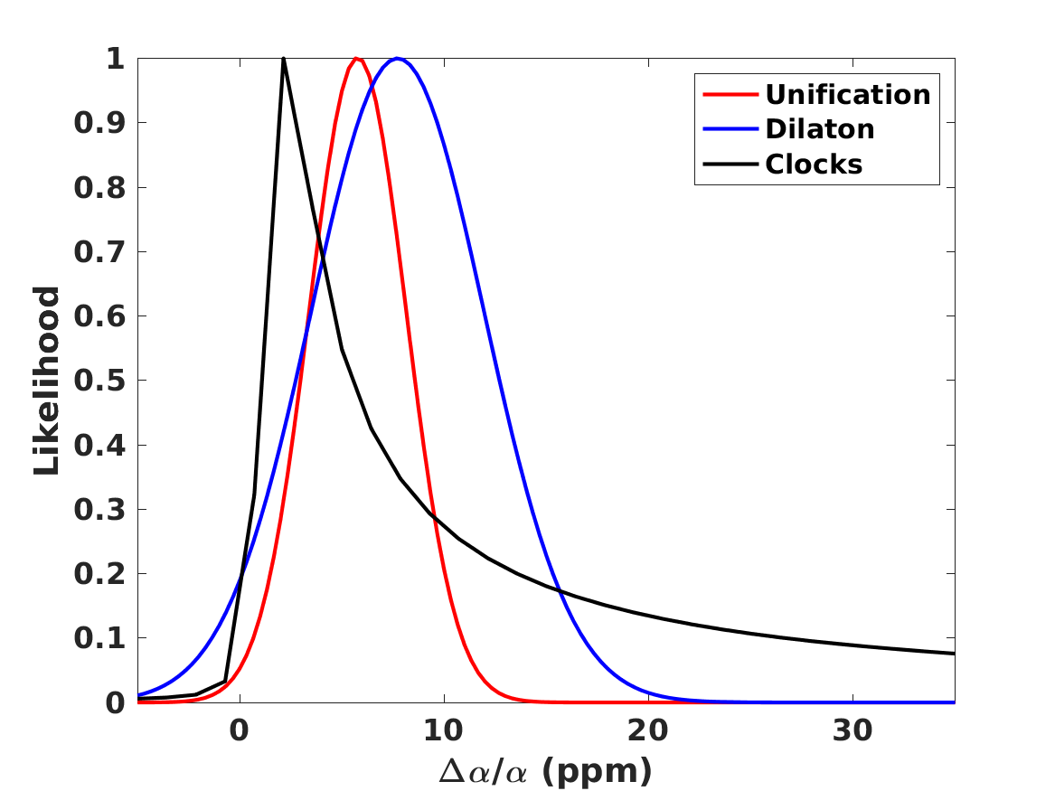
We now repeat the statistical likelihood analysis, allowing for both a variation of fundamental couplings and lithium-7 depletion, for these three models. In this section we assume that the values of the number of neutrino species and the baryon-to-photon ratio are fixed at their standard fiducial values, but the neutron lifetime is implicitly allowed to vary, as pointed out above. The results of this analysis are depicted in Figure 2 and also summarized in Table 5 for the Baseline case; naturally, in the Null case the depletion fraction is unconstrained, but for comparison we also list the value of in that case.
| Parameter | Unification | Dilaton | Clocks |
| (ppm), Null | |||
| (ppm), Baseline | |||
| (Cos) | |||
| (Ast) |
The observed BBN abundances allow the separate quantification of the role of both effects. We see that the preferred value of the depletion parameter decreases with respect to the one obtained with the standard value of in Section 2, by about one standard deviation. Moreover, there is still a preference for a positive value of . Comparison with Table 4 shows that for the Unification and Dilaton models both the best-fit values and the statistical significance of the preference for the Baseline case are decreased with respect to the values found in Paper 1 and Paper 2, while for the Null case they are slightly increased. On the other hand, for the Clocks model the best-fit value for is in agreement with the one found in Paper 1 and Paper 2 in both the Null and the Baseline cases. In this case the effect of the additional depletion mechanism is manifest in the best-fit values for the phenomenological particle physics parameters and . Here we find
| (24) |
whereas in Paper 2 the best-fit values were
| (25) |
Note that although and are independent parameters in the likelihood analysis, the local prior from atomic clock experiments—cf. Equation (23)—effectively correlates them. The difference between the two sets of values reflects the fact that in Paper 2 there was no allowance for a depletion factor (effectively, was used). Moreover, bearing in mind the aforementioned slight reduction of the depletion factor when a non-standard value of is allowed, it also shows that although a value of does alleviate the lithium problem, it does not completely solve it. Instead, a significant depletion factor is still statistically preferred.
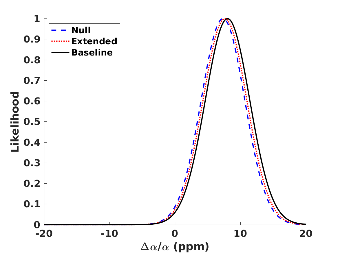
The more noteworthy aspect is that, unlike the results of Paper 1 and Paper 2, the preferred values for are almost identical in the Baseline and Null cases, meaning that the preference for a positive value of is not driven by the lithium-7 problem. In other words, even without including lithium-7 in the analysis, there is a mild statistical preference for a variation of at the few parts-per-million level. Instead, it is driven by the small discrepancy, already mentioned in the previous section, between the baryon-to-photon ratios inferred from BBN and the corresponding CMB value; in other words, it is driven by the helium-4 and deuterium data. We note that within the standard paradigm the baryon-to-photon ratio is a constant, having the same value at the BBN and CMB epochs; a different value at the two epochs necessarily implies the presence of new physics.
When adding lithium-7 to the analysis without allowing for the possibility of a depletion mechanism (as was done in Paper 1 and Paper 2) the preferred value of increases very significantly with respect to the Null case, since a larger value of is needed solve the lithium problem per se. On the other hand, if a depletion mechanism is allowed (as in the present work) then this mechanism provides the dominant contribution to address the lithium problem, and the value of is very slightly changed with the respect to the null case. Nevertheless the inclusion of is still significant, which is manifest in the fact that the preferred depletion fraction changes with respect to the case discussed in the previous section by about one standard deviation.
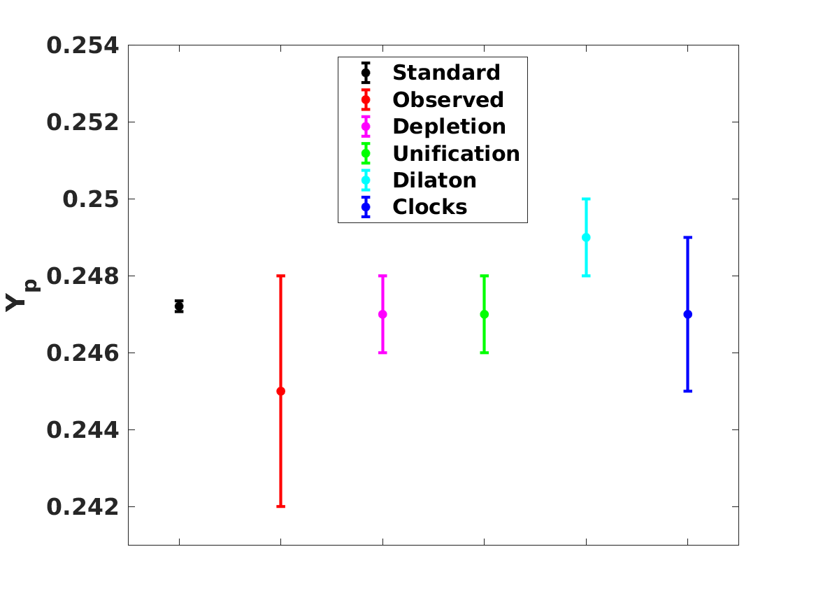
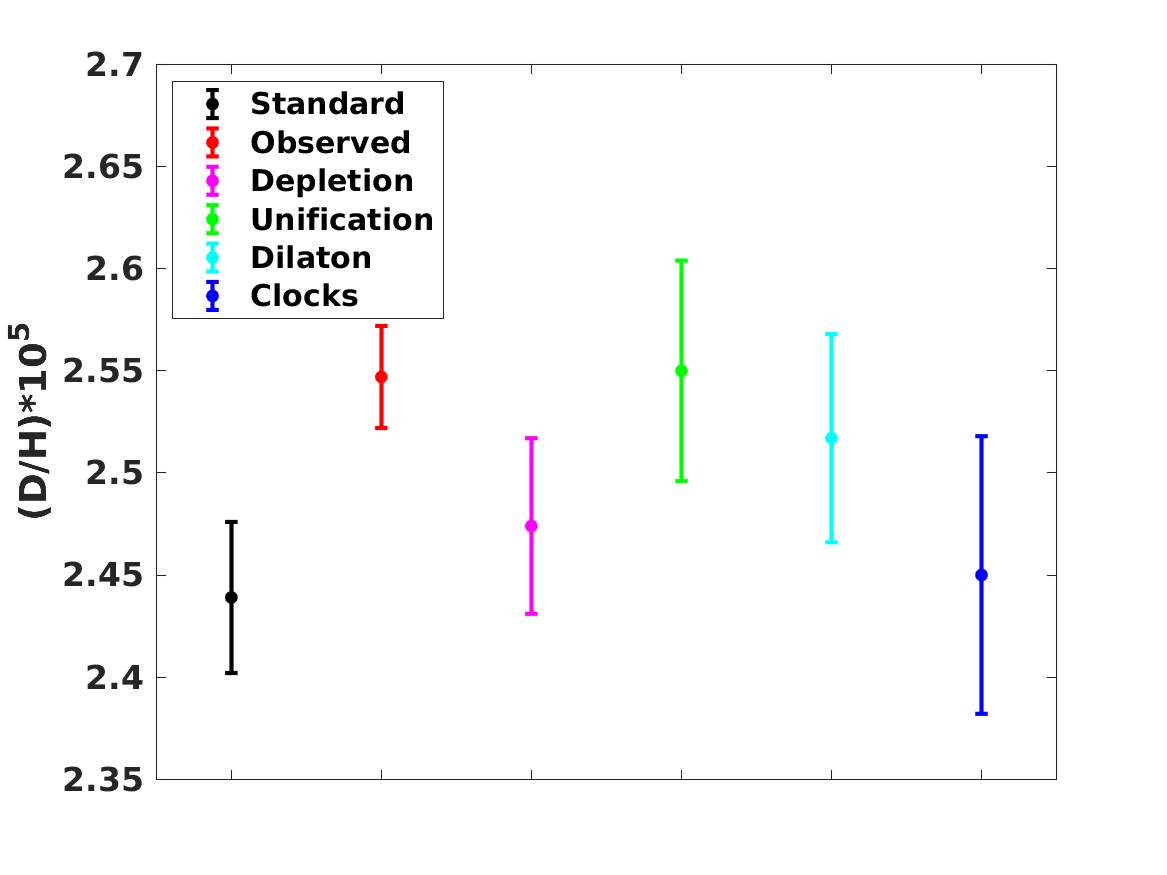
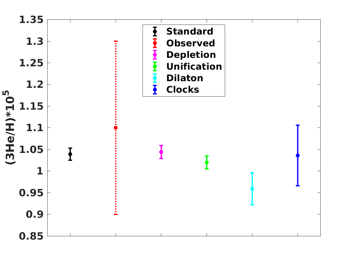
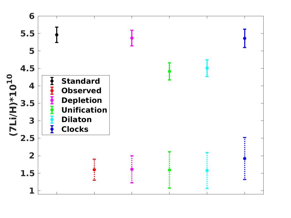
A summary plot of the standard theoretical and observed abundances, together with those predicted for the best-fit values of the various models discussed both in Section 2 and in the present one, can be found in Figure 3.
It is interesting to note that although the Unification and Dilaton models lead to very similar lithium-7 abundances (a consequence of the fact that this nuclide drives the statistical analysis), they lead to significantly different ones for the other nucildes, especially helium-4 and helium-3. Specifically, the Dilaton model leads to a significantly higher helium-4 abundance and a significantly lower helium-3 abundance, as compared to the Unification model. This is due to the fact that in the Dilaton model, where is comparatively large, there are large positive and negative sensitivity coefficients, respectively for helium-4 and helium-3. The comparison between the three models also confirms the well-known result that, for the observationally relevant ratios of the baryon-to-photon ratio, the deuterium and lithium-7 abundances are anticorrelated (Olive et al., 2012; Coc et al., 2015), so a reduction of the latter abundance leads to an increase of the former. Similarly, one can notice an anticorrelation between the helium-4 and helium-3 abundances, highlighting the fact that an accurate determination of the primordial cosmological abundance would provide a sensitive consistency test of BBN.
4 Stellar depletion and the Lithium problem
In this section we assess how realistic is the depletion factor , determined in the previous Section, according to stellar evolution theory. We compare to predicted lithium-7 depletion in stellar models, including different transport processes of chemical elements.
4.1 Input physics of the stellar models
The depletion of lithium that occurs during the evolution of Population II stars is predicted using the Montreal/Montpellier stellar evolution code (Turcotte et al., 1998b) and Code d’Evolution Stellaire Adatpatif et Modulaire (CESTAM, the ”T” stands for Transport: Morel & Lebreton 2008, Marques et al. 2013, Deal et al. 2018). We used two stellar evolution codes firstly for confirmation of the results, and secondly because they do not include the same transport processes of chemical elements. The Montréal/Montpellier code has already been used to model Population II stars, and especially lithium surface abundances, including detailed atomic diffusion calculations (e.g. Richard et al., 2005). The CESTAM evolution code also includes atomic diffusion (with independent formalisms, see Deal et al. 2018 for more details) and is able to model the effect of rotation (Marques et al., 2013).
Our Montréal/Montpellier models have the same input physics as the ones used by Deal et al. (2021) without accretion. CESTAM models are computed with the same input physics as in Deal et al. (2020), except for the mixing length parameter set to following the Canuto et al. (1996) formalism. The opacity tables are the OP table at fixed chemical composition and not the monochromatic ones (OPCDv3.3, Seaton, 2005). We tested that with the additional transport processes included in the models, the abundance variation are not sufficient to modify the internal structure (especially the size of the surface convective zone). Using simpler opacity tables has then a negligible impact of the lithium surface abundance in the specific framework of this study111Such an approximation of the opacity calculation in presence of transport of chemical elements is not valid in most cases (e.g. Turcotte et al., 1998a; Richard et al., 2001; Théado et al., 2009; Deal et al., 2016, 2018).. No core overshoot is taken into account and the initial chemical composition is the one of Montréal/Montpellier models ([Fe/H] dex). Considering a wider range of initial chemical composition would not affect the conclusion of this work, because at these low metallicities the structure variations are small (especially the size of the surface convective zone, which is important for lithium surface abundances variations, see e.g. Richard et al. 2002). It should be noticed that, with such models, there is no extra depletion/dispersion for the lower metallicities, as it has been observed (Sbordone et al., 2010). The mechanism to explain this behavior is still unknown. The models are computed with masses between 0.55 and 0.78 . All models are on the main sequence at 12.5 Gyr and cover a range of effective temperature [5000,6500] K, typical of observed main-sequence Population II stars. The physics of all models is presented in Table 6.
| Code | Montréal/Montpellier$a$$a$footnotetext: | CESTAM$b$$b$footnotetext: | ||||||
|---|---|---|---|---|---|---|---|---|
| Model set | 1 | 2 | 3 | 4 | 5 | 6 | 7 | 8 |
| [ K]$1$$1$footnotetext: | 1.0, 1.32, 1.74, 1.80, 1.90, 2.24 | 1.60, 1.74, 1.80, 1.90 | - | - | - | - | - | - |
| [km.-1] | - | - | ||||||
| [cm2.s-1] | - | - | ||||||
| [] | - | - | - | - | ||||
| Opacities | OPAL monochromatic$c$$c$footnotetext: | OP$d$$d$footnotetext: | ||||||
| Eos | CEFF$e$$e$footnotetext: | OPAL2005$f$$f$footnotetext: | ||||||
| Nuc. react. | Bahcall92$g$$g$footnotetext: | NACRE+LUNA$h$$h$footnotetext: | ||||||
| 1.66$i$$i$footnotetext: | 0.69$j$$j$footnotetext: | |||||||
| Initial mix. | AGSS09$k$$k$footnotetext: | |||||||
| (7Li/H) | ||||||||
| [Fe/H] | ||||||||
| enhanc. | ||||||||
| Core ov. | none | |||||||
4.2 Transport processes of chemical elements
We computed stellar models including different transport processes of chemical elements. In particular, they all affect the transport of lithium-7 and therefore play a role in the lithium depletion. Most of the processes considered in this study were extensively described by Dumont et al. (2020), and references therein. In the following, we briefly describe the impact of the processes on lithium depletion and the prescriptions we use in the stellar models. As the aim of this section is to show that the depletion factor can be explained by stellar physics, we only included simple modelling approaches for some of the processes addressed below. Including more realistic modelling is the next natural step of this study.
Convection:
All models include convection using the Schwarzschild criterion. In convective zones, the transport of chemical elements is very efficient and fully homogenizes the chemical composition. If the bottom part of the convective zone has a temperature close to or larger than the temperature at which lithium is destroyed by proton capture ( K), lithium is efficiently depleted. Convective boundaries are defined by the Schwarzschild criterion (Schwarzschild, 1958) (or Ledoux criterion, Ledoux 1947) in stellar models. It has been shown than convective plumes can penetrate the radiative zone and then extend the mixing of chemical elements beyond the standard convection criteria (e.g. Zahn, 1991; Baraffe et al., 2017). If this extension of the mixing reaches the region where lithium is destroyed by proton capture, this will also lead to lithium depletion. For the models in this study, we include a simple constant step extension of the surface convective zone in pressure scale height units (). More sophisticated approach exist (see Dumont et al., 2020, for an overview).
Atomic diffusion:
All models also include atomic diffusion, which is a selective microscopic transport process. It occurs in every star and it the consequence of the internal gradients of pressure, temperature and concentration (Michaud et al., 2015). It is efficient in radiative zones. This is mainly the competition between gravity, which makes elements move toward the center of stars, and radiative acceleration, which makes elements move toward the surface of stars. For the stellar models used in this study, radiative acceleration on lithium is negligible. The transport of lithium by atomic diffusion is dominated by the gravitational settling.
Parametrized turbulent diffusion coefficient:
Atomic diffusion alone cannot explain the lithium surface abundance of star. There is a need to include competing transport processes. It is possible to account for them using a parametrized turbulent diffusion coefficient. Such a coefficient was already used and calibrated to reproduce the lithium surface abundance in Population II stars (Richard et al., 2005; Deal et al., 2021) and in clusters (e.g. Gruyters et al., 2013, 2016; Korn et al., 2007). The turbulent diffusion coefficient is expressed as:
| (26) |
where is a reference temperature. is the diffusion coefficient of helium at the reference point333The diffusion coefficient of helium can be easily calculated using this approximate formula: , the local density and the density at the reference point. The only free parameter of this parametrization is . The way this parametrization is made, the transport of chemical elements is very efficient for internal temperatures smaller than (i.e. the chemical composition is homogenized from the surface down to ). For temperatures larger than the mixing decreases rapidly as a function of . The larger is , the deeper goes the efficient mixing region.
Rotational-induced mixing:
The transport of chemical elements induced by rotation is one of the processes in competition with atomic diffusion. It has an important impact on chemical elements and especially on lithium (e.g. Charbonnel & Talon, 1999; Talon, 2008; Dumont et al., 2020). Rotational-induced mixing is mainly driven by the shear instability and the meridional circulation. The differences between the models of this study and the ones of Deal et al. (2020) are the horizontal diffusion coefficient (, from Mathis et al. 2018) and an additional vertical viscosity cm2s-1 as calibrated by Ouazzani et al. (2019) to take into account the fact that the current rotation theory underestimates the transport of angular momentum. We also tested smaller values of . All models including rotation have a rotation speed at the ZAMS km.-1. See Marques et al. (2013) for a detailed description of the modelling of rotation in CESTAM.
4.3 Parametrized turbulent transport and atomic diffusion
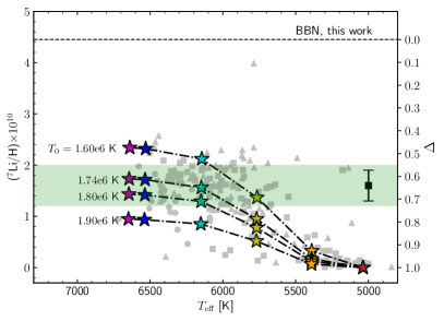
We first estimate the required transport of chemical elements to explain the depletion factor, using the parametric turbulent diffusion described in Section 4.2 and atomic diffusion. This kind of approach has already been used to study lithium surface abundances of Population II stars (e.g. Richard et al., 2005; Deal et al., 2021).
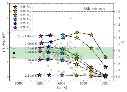
The left panel of Fig. 4, shows the lithium surface abundance at 12.5 Gyr in stellar models computed with the Montréal/Montpellier stellar evolution code, including atomic diffusion and different parametrizations of the turbulent diffusion coefficient (models set 1). The models are computed with an initial primordial lithium abundance (7Li/H)= 4.45, following the values of Table 5 for the Unification and Dilaton models. Lithium depletion is larger for the smaller masses because of a deeper surface convective zone, i.e. close to the region where lithium is destroyed by nuclear reactions. The larger the value, the deeper the turbulent mixing, leading to stronger depletion. The smaller the value, the stronger are the effect of atomic diffusion, i.e. the turbulent mixing is not strong enough to balance it. This is the reason why for K, the depletion is larger at 0.78 than 0.65 . We see that observations, as well as the range of values previously determined, are well reproduced by the models, for the whole effective temperature range, for values between and K.
The CESTAM models (right panel of Fig. 4, models set 2), show similar surface abundances, with a slight shift in the values and in effective temperatures. This difference comes from the different input physics (including the equation of state, opacity tables, and nuclear reaction rates) between the two stellar evolution codes. At a given value, the difference in lithium abundance is about 10% at maximum, which will not impact the conclusion of this study. This justifies our confidence in using CESTAM models. In the following subsections, we will estimate what are the possible physical processes responsible for such turbulent transport.
4.4 Rotationally-induced mixing and atomic diffusion
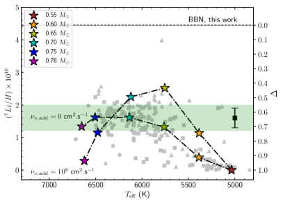
In this section we assess whether the depletion factor is linked to the combination of rotational induced-mixing and atomic diffusion. Figure 5 shows two sets of models (sets 3 and 4) in which the two processes are included. In one case, rotation is almost solid (set 3, with cm2s-1) and in the other case the internal rotation is differential using the standard theory for rotation (set 4, with cm2s-1). The models with an internal differential rotation are in very good agreement with the observations. We tested larger initial rotation speeds for the models with quasi-solid rotation and the results are very similar. The rotation speed does not play a major role for the transport of chemicals in this specific case.
Helio/Asteroseismology (study of oscillation of the Sun/stars) also allows us to probe the internal rotation of stars. It has been shown that the internal rotation of the Sun is nearly uniform in the radiative zone at least down to (e.g. Kosovichev, 1988; García et al., 2007). Solar models accounting for standard rotation predict a high degree of radial differential rotation (e.g. Eggenberger et al., 2005). The same conclusions are reached when comparing other stars for which we can access the core rotation (e.g. Tayar & Pinsonneault, 2013; Deheuvels et al., 2014; Ouazzani et al., 2019). This indicates that among sets 3 and 4, the more realistic models are those of set 3. This implies that the lithium surface abundances of Population II cannot be explained by the combined effect of atomic diffusion and rotation. The same kind of conclusion have been previously obtained for other types of stars (e.g. Deal et al., 2020).
4.5 Penetrative convection, rotationally-induced mixing and atomic diffusion
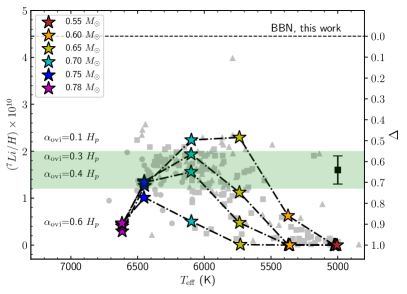
In this section we assess whether the depletion factor can be accounted for by the combination of penetrative convection, rotational induced-mixing and atomic diffusion. Figure 6 shows four sets of models (set 5, 6, 7 and 8) in which the three processes are included. We see that the four sets cover well the range of observed lithium surface abundances up to an effective temperature of about K. The values of penetrative convection considered in the models are consistent with what has been determined for the Sun (, Christensen-Dalsgaard et al. 2011). For the hotter (more massive) stars, an additional transport process is probably needed to reduce the lithium depletion induced by atomic diffusion. It is possible that the amount of penetrative convection is larger for the more massive stars, which could also make the models agree better with the observation. A more realistic treatment of this process could also improve the agreement. Note that penetrative convection was also invoked in an other scenario to explain lithium abundances in Population II stars (e.g. Fu et al., 2015).
4.6 A minimum astrophysical depletion?
It is interesting to note that there is a minimum depletion obtained in the models presented in Section 4.5, which is around . From the stellar modelling point of view, the transport process with the more accurate modelling and leading to the smallest lithium depletion (for masses around 0.60-0.70 M⊙) is atomic diffusion. The efficiency of atomic diffusion strongly depends on the internal structure of stars, and especially on the size of the surface convective zone. The prediction of the minimum depletion of lithium, expected from stellar models including atomic diffusion only, is then subject to the input physics of the models (including opacity tables, equations of state, convection theory, nuclear reaction rates, etc.). This is less the case when other competing transport processes are taken into account (see the comparison done in Fig. 4). In this context, it is difficult to provide a strong constrain on the minimum lithium depletion expected from stellar models. As an example, for the input physics considered in this paper, we find for models including atomic diffusion only. The only robust conclusion we can draw at this point is that in all models including expected transport processes (i.e. at least atomic diffusion).
Overall, we have shown that lithium surface abundances of Population II stars, as well as the range of values determined in Section 3, are well reproduced by models including atomic diffusion, a nearly uniform rotation, and some amount of penetrative convection convection, even if our modelling of the latter and of the missing transport of angular momentum has been somewhat simple. A more realistic modelling of these processes, and a systematic study of the effect of the different input physics (opacity tables, equation of states, convection theory, nuclear reaction rates, etc.), are needed to drawn stronger conclusions, but our work suffices to show that transport processes of chemical elements in stars not only need to be considered when addressing the lithium problem, but also are very probable candidates to solve it.
5 Varying fundamental constants and the Deuterium discrepancy
Having previously identified the small discrepancy between the baryon-to-photon ratios inferred from BBN and the CMB value as the origin of the preference for a non-standard value of , here we assess the relative contributions of the helium-4 and deuterium data to this result.
To this end, we repeat the analysis both for the case where only the deuterium abundance is used and for the case where both deuterium and helium-4 are used. For each of these we further consider two sub-cases, ether keeping the cosmological parameters (i.e., the neutron lifetime, number of neutrinos and baryon-to-photon ratio) fixed at their best-fit values introduced in Sect. 2, or letting these parameters vary (with the previously described priors) and then marginalizing them.
In the former case, the parameter space is summarized by Eq. 19 and the relevant sensitivity coefficients are given in Table 3. In the latter case the parameter space is wider:
| (27) |
As previously mentioned, a variation of itself impacts the neutron lifetime; unlike in Sect. 3, here we explicitly separate this effect from the rest of the effects of the variation. This means that the -related sensitivity coefficients will change, and we have highlighted this point by adding the subscript in the previously defined sensitivity coefficients , and . For completeness, all these sensitivity coefficients are reproduced in Table 7.
| D | 3He | 4He | 7Li | |
|---|---|---|---|---|
| +42.1 | +1.30 | -4.5 | -166.5 | |
| +40.1 | +2.00 | -3.5 | -150.7 | |
| +34.9 | -90.0 | +11.8 | -202.6 | |
| +0.442 | +0.141 | +0.732 | +0.438 | |
| +0.409 | +0.136 | +0.164 | -0.277 | |
| -1.65 | -0.567 | +0.039 | +2.08 |
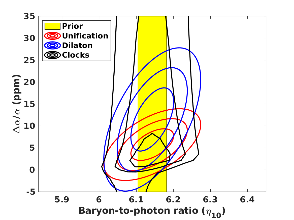
The results of our analysis with the deuterium and helium-4 abundances are summarized in Figure 7 and Table 8; the latter can be usefully compared with the Baseline and Null cases reported in Table 5.
| Data | Parameters | Unification | Dilaton | Clocks |
|---|---|---|---|---|
| D only | Fixed | |||
| D only | Marginalized | |||
| D He4 | Fixed | |||
| D He4 | Marginalized |
First and foremost, we confirm that the preference for is driven by the Deuterium results, and the top panels of Figure 7 also makes it clear that this is due to the positive correlation between and the baryon-to-photon ratio , though the strength of this correlation is model-dependent. Secondly, we find that the Helium-4 abundance plays a relatively minor role, though one that again depends on the assumed model.
Specifically, for the Unification and Clocks model, the results in Table 8 are fully consistent with the ones for the previously discussed Baseline and Null cases. The positive correlation between and is relatively mild, In these circumstances helium-4 does not noticeably affect the constraints on , while allowing the cosmological parameters to vary and marginalizing them simply increases the statistical uncertainties, and therefore decreases the significance of the preference.
On the other hand, for the Dilaton model the results are more sensitive to the assumptions underlying the analysis. On the one hand, the stronger positive correlation between and means that whether or not is allowed to vary has a mild but discernible impact even in the case where only deuterium is used in the analysis. On the other hand, the inclusion of helium-4 significantly lowers the preferred value of , the reason being that this model tends to overpredict the helium-4 abundance, as can bee seen in Figure 3. Again, this shows the potential of BBN as a precision test of these theoretical scenarios.
6 Conclusions
We have provided an updated analysis of BBN constraints in the framework of a wide class of Grand Unified Theory scenarios (Clara & Martins, 2020; Martins, 2021), in particular addressing the long-standing Lithium problem (Fields, 2011; Mathews et al., 2020) and the more recently noticed Deuterium discrepancy (Pitrou et al., 2021). For the former we have highlighted and quantified the astrophysical mechanisms that can provide a solution, while for the latter we have identified a possible hint of new physics, specifically a mild (two to three standard deviations) preference for , at the parts per million level. Such variations would be consistent with all other current constraints (Martins, 2017).
We note that the Deuterium discrepancy identified by Pitrou et al. (2021) is not found by other authors (Yeh et al., 2021; Pisanti et al., 2021), who rely on different reaction rates. From a statistical point of view, the main difference is that the uncertainties in the theoretical abundances obtained by Pitrou et al. (2021) are smaller than those of other analyses, although there are also small differences in the preferred values of these abundances. While we have not repeated our analysis with these different reaction rates (and the corresponding theoretical abundances inferred from them) we would expect that the propagation of the larger uncertainties on the theoretical side would lead to larger uncertainties on the fine-structure constant measurements, reducing the statistical significance of the preference for a non-standard value.
We have quantitatively determined the amount a lithium depletion needed to solve the lithium problem and searched for depletion mechanisms occurring during the evolution of stars, namely, the transport processes of chemical elements. We have shown that taking into account, in stellar models, atomic diffusion, rotational-induced mixing and some amount of penetrative convection (consistent with the amount determined from solar observation, Christensen-Dalsgaard et al. 2011), allows us to reproduce the lithium surface abundances of Population II stars. More realistic modelling of some of the processes (especially the penetrative convection, and the missing transport of angular momentum) are required to draw a more robust conclusion, but this work shows the necessity of including the stellar contribution to the lithium problem. Transport processes of chemical elements are most likely the dominant contribution to the solution to this problem.
The stellar models were computed with the best fit value for the initial primordial lithium abundance derived in this study, in the context of the GUT scenarios under consideration, of approximately (7Li/H). Considering stellar models with a larger initial primordial lithium, as obtained in the standard BBN model (i.e. (7Li/H)) would not strongly impact our conclusions. This difference would only lead to the need of a slightly larger amount of penetrative convection to explain the extra depletion. This also shows that from the stellar physics point of view, the accuracy of the primordial lithium abundance is crucial to constrain the transport of chemical elements in metal poor stars.
It is worthy of note that currently there are only two primordial (cosmological) abundances that are well known, those of Deuterium and Helium-4. It is therefore highly desirable to close the loop through a cosmological measurement of the Helium-3 abundance, especially given the anticorrelation between the helium-4 and helium-3 abundances. This would enable a key consistency test of the underlying physics, which will be particularly crucial should evidence for new physics be confirmed.
Our analysis highlights the role of BBN as consistency test of the standard cosmological paradigm, and as a sensitive probe of new physics. For the broad phenomenological but physically motivated class of models we have considered, improving the observed abundances of Deuterium and Helium-4 by a factor of 2-3 will provide a stringent test, and in particular will definitively confirm or rule out the present tentative evidence for the variation. This is a highly compelling science case for the forthcoming Extremely Large Telescope (Liske et al., 2014; Marconi et al., 2020), provided it has an efficient blue wavelength coverage.
Acknowledgements.
This work was supported by FCT—Fundação para a Ciência e a Tecnologia through national funds (grants PTDC/FIS-AST/28987/2017 and PTDC/FIS-AST/30389/2017) and by FEDER—Fundo Europeu de Desenvolvimento Regional funds through the COMPETE 2020—Operacional Programme for Competitiveness and Internationalisation (POCI-01-0145-FEDER-028987 and POCI-01-0145-FEDER-030389). Additional funds were provided by FCT/MCTES through the research grants UIDB/04434/2020 and UIDP/04434/2020. MD is supported by national funds through FCT in the form of a work contract. CJM gratefully acknowledges useful discussions with Brian Fields and Cyril Pitrou in the context of the ESO Cosmic Duologue on BBN, and with Paolo Molaro. We thank an anonymous referee for valuable comments which helped to improve the paper.References
- Aghanim et al. (2020) Aghanim, N. et al. 2020, Astron. Astrophys., 641, A6
- Aguado et al. (2019) Aguado, D. S., Hernández, J. I. G., Allende Prieto, C., & Rebolo, R. 2019, Astrophys. J. Lett., 874, L21
- Angulo (1999) Angulo, C. 1999, in American Institute of Physics Conference Series, Vol. 495, American Institute of Physics Conference Series, 365–366
- Asplund et al. (2009) Asplund, M., Grevesse, N., Sauval, A. J., & Scott, P. 2009, ARA&A, 47, 481
- Aver et al. (2015) Aver, E., Olive, K. A., & Skillman, E. D. 2015, JCAP, 1507, 011
- Bahcall & Pinsonneault (1992) Bahcall, J. N. & Pinsonneault, M. H. 1992, Reviews of Modern Physics, 64, 885
- Bania et al. (2002) Bania, T. M., Rood, R. T., & Balser, D. S. 2002, Nature, 415, 54
- Baraffe et al. (2017) Baraffe, I., Pratt, J., Goffrey, T., et al. 2017, ApJ, 845, L6
- Böhm-Vitense (1958) Böhm-Vitense, E. 1958, ZAp, 46, 108
- Bonifacio & Molaro (1997) Bonifacio, P. & Molaro, P. 1997, MNRAS, 285, 847
- Bonifacio et al. (2007) Bonifacio, P., Molaro, P., Sivarani, T., et al. 2007, A&A, 462, 851
- Brown et al. (2013) Brown, J. M., Garaud, P., & Stellmach, S. 2013, ApJ, 768, 34
- Campbell & Olive (1995) Campbell, B. A. & Olive, K. A. 1995, Phys.Lett., B345, 429
- Canuto et al. (1996) Canuto, V. M., Goldman, I., & Mazzitelli, I. 1996, ApJ, 473, 550
- Cayrel et al. (2008) Cayrel, R., Steffen, M., Bonifacio, P., Ludwig, H. G., & Caffau, E. 2008, in Nuclei in the Cosmos (NIC X), E2
- Charbonnel & Talon (1999) Charbonnel, C. & Talon, S. 1999, A&A, 351, 635
- Charbonnel et al. (1994) Charbonnel, C., Vauclair, S., Maeder, A., Meynet, G., & Schaller, G. 1994, A&A, 283, 155
- Christensen-Dalsgaard & Daeppen (1992) Christensen-Dalsgaard, J. & Daeppen, W. 1992, A&A Rev., 4, 267
- Christensen-Dalsgaard et al. (2011) Christensen-Dalsgaard, J., Monteiro, M. J. P. F. G., Rempel, M., & Thompson, M. J. 2011, MNRAS, 414, 1158
- Clara & Martins (2020) Clara, M. & Martins, C. 2020, Astron. Astrophys., 633, L11
- Coc et al. (2007) Coc, A., Nunes, N. J., Olive, K. A., Uzan, J.-P., & Vangioni, E. 2007, Phys.Rev., D76, 023511
- Coc et al. (2015) Coc, A., Petitjean, P., Uzan, J.-P., et al. 2015, Phys. Rev. D, 92, 123526
- Cooke et al. (2018) Cooke, R. J., Pettini, M., & Steidel, C. C. 2018, Astrophys. J., 855, 102
- Damour et al. (2002) Damour, T., Piazza, F., & Veneziano, G. 2002, Phys. Rev. Lett., 89, 081601
- Deal et al. (2018) Deal, M., Alecian, G., Lebreton, Y., et al. 2018, A&A, 618, A10
- Deal et al. (2020) Deal, M., Goupil, M. J., Marques, J. P., Reese, D. R., & Lebreton, Y. 2020, A&A, 633, A23
- Deal et al. (2016) Deal, M., Richard, O., & Vauclair, S. 2016, A&A, 589, A140
- Deal et al. (2021) Deal, M., Richard, O., & Vauclair, S. 2021, arXiv e-prints, arXiv:2101.01522
- Deheuvels et al. (2014) Deheuvels, S., Doğan, G., Goupil, M. J., et al. 2014, A&A, 564, A27
- Denissenkov (2010) Denissenkov, P. A. 2010, ApJ, 723, 563
- Dent et al. (2007) Dent, T., Stern, S., & Wetterich, C. 2007, Phys.Rev., D76, 063513
- Dumont et al. (2020) Dumont, T., Palacios, A., Charbonnel, C., et al. 2020, arXiv e-prints, arXiv:2012.03647
- Eggenberger et al. (2005) Eggenberger, P., Maeder, A., & Meynet, G. 2005, A&A, 440, L9
- Ferreira et al. (2012) Ferreira, M. C., Juliao, M. D., Martins, C. J. A. P., & Monteiro, A. M. R. V. L. 2012, Phys.Rev., D86, 125025
- Fields (2011) Fields, B. D. 2011, Ann. Rev. Nucl. Part. Sci., 61, 47
- Flambaum & Wiringa (2007) Flambaum, V. V. & Wiringa, R. B. 2007, Phys. Rev., C76, 054002
- Fu et al. (2015) Fu, X., Bressan, A., Molaro, P., & Marigo, P. 2015, MNRAS, 452, 3256
- García et al. (2007) García, R. A., Turck-Chièze, S., Jiménez-Reyes, S. J., et al. 2007, Science, 316, 1591
- Gruyters et al. (2013) Gruyters, P., Korn, A. J., Richard, O., et al. 2013, A&A, 555, A31
- Gruyters et al. (2016) Gruyters, P., Lind, K., Richard, O., et al. 2016, A&A, 589, A61
- Iglesias & Rogers (1996) Iglesias, C. A. & Rogers, F. J. 1996, ApJ, 464, 943
- Iliadis & Coc (2020) Iliadis, C. & Coc, A. 2020, Astrophys. J., 901, 127
- Imbriani et al. (2004) Imbriani, G., Costantini, H., Formicola, A., et al. 2004, A&A, 420, 625
- Iocco et al. (2009) Iocco, F., Mangano, G., Miele, G., Pisanti, O., & Serpico, P. D. 2009, Phys. Rept., 472, 1
- Korn et al. (2006) Korn, A. J., Grundahl, F., Richard, O., et al. 2006, Nature, 442, 657
- Korn et al. (2007) Korn, A. J., Grundahl, F., Richard, O., et al. 2007, ApJ, 671, 402
- Kosovichev (1988) Kosovichev, A. G. 1988, Soviet Astronomy Letters, 14, 145
- Langacker et al. (2002) Langacker, P., Segre, G., & Strassler, M. J. 2002, Phys. Lett., B528, 121
- Ledoux (1947) Ledoux, P. 1947, ApJ, 105, 305
- Liske et al. (2014) Liske, J., Bono, G., Cepa, J., et al. 2014, Top Level Requirements For ELT-HIRES, Tech. rep., Document ESO 204697 Version 1
- Maeder (2009) Maeder, A. 2009, Physics, Formation and Evolution of Rotating Stars
- Marconi et al. (2020) Marconi, A., Abreu, M., Adibekyan, V., et al. 2020, in Society of Photo-Optical Instrumentation Engineers (SPIE) Conference Series, Vol. 11447, Society of Photo-Optical Instrumentation Engineers (SPIE) Conference Series, 1144726
- Marques et al. (2013) Marques, J. P., Goupil, M. J., Lebreton, Y., et al. 2013, A&A, 549, A74
- Martins (2017) Martins, C. J. A. P. 2017, Rep. Prog. Phys., 80, 126902
- Martins (2021) Martins, C. J. A. P. 2021, Astron. Astrophys., 646, A47
- Mathews et al. (2020) Mathews, G., Kedia, A., Sasankan, N., et al. 2020, JPS Conf. Proc., 31, 011033
- Mathis et al. (2018) Mathis, S., Prat, V., Amard, L., et al. 2018, A&A, 620, A22
- Michaud et al. (2015) Michaud, G., Alecian, G., & Richer, J. 2015, Atomic Diffusion in Stars
- Michaud et al. (1984) Michaud, G., Fontaine, G., & Beaudet, G. 1984, ApJ, 282, 206
- Morel & Lebreton (2008) Morel, P. & Lebreton, Y. 2008, Ap&SS, 316, 61
- Mossa et al. (2020) Mossa, V. et al. 2020, Nature, 587, 210
- Muller et al. (2004) Muller, C. M., Schafer, G., & Wetterich, C. 2004, Phys.Rev., D70, 083504
- Nakashima et al. (2010) Nakashima, M., Ichikawa, K., Nagata, R., & Yokoyama, J. 2010, JCAP, 1001, 030
- Olive et al. (2012) Olive, K. A., Petitjean, P., Vangioni, E., & Silk, J. 2012, Mon. Not. Roy. Astron. Soc., 426, 1427
- Ouazzani et al. (2019) Ouazzani, R. M., Marques, J. P., Goupil, M. J., et al. 2019, A&A, 626, A121
- Palacios et al. (2003) Palacios, A., Talon, S., Charbonnel, C., & Forestini, M. 2003, A&A, 399, 603
- Pisanti et al. (2021) Pisanti, O., Mangano, G., Miele, G., & Mazzella, P. 2021, JCAP, 04, 020
- Pitrou et al. (2018) Pitrou, C., Coc, A., Uzan, J.-P., & Vangioni, E. 2018, Phys. Rept., 754, 1
- Pitrou et al. (2021) Pitrou, C., Coc, A., Uzan, J.-P., & Vangioni, E. 2021, Mon. Not. Roy. Astron. Soc., 502, 2474
- Rajan & Desai (2020) Rajan, A. & Desai, S. 2020, PTEP, 2020, 013C01
- Richard et al. (2001) Richard, O., Michaud, G., & Richer, J. 2001, ApJ, 558, 377
- Richard et al. (2002) Richard, O., Michaud, G., & Richer, J. 2002, ApJ, 580, 1100
- Richard et al. (2005) Richard, O., Michaud, G., & Richer, J. 2005, ApJ, 619, 538
- Rogers & Nayfonov (2002) Rogers, F. J. & Nayfonov, A. 2002, ApJ, 576, 1064
- Ryan et al. (2000) Ryan, S. G., Beers, T. C., Olive, K. A., Fields, B. D., & Norris, J. E. 2000, Astrophys. J. Lett., 530, L57
- Sbordone et al. (2010) Sbordone, L., Bonifacio, P., Caffau, E., et al. 2010, A&A, 522, A26
- Schwarzschild (1958) Schwarzschild, M. 1958, Structure and evolution of the stars.
- Seaton (2005) Seaton, M. J. 2005, MNRAS, 362, L1
- Spite & Spite (1982) Spite, F. & Spite, M. 1982, A&A, 115, 357
- Stancliffe (2009) Stancliffe, R. J. 2009, MNRAS, 394, 1051
- Steigman (2007) Steigman, G. 2007, Ann. Rev. Nucl. Part. Sci., 57, 463
- Suda et al. (2017) Suda, T., Hidaka, J., Aoki, W., et al. 2017, PASJ, 69, 76
- Suda et al. (2008) Suda, T., Katsuta, Y., Yamada, S., et al. 2008, PASJ, 60, 1159
- Suda et al. (2011) Suda, T., Yamada, S., Katsuta, Y., et al. 2011, MNRAS, 412, 843
- Talon (2008) Talon, S. 2008, Mem. Soc. Astron. Italiana, 79, 569
- Tayar & Pinsonneault (2013) Tayar, J. & Pinsonneault, M. H. 2013, ApJ, 775, L1
- Théado et al. (2009) Théado, S., Vauclair, S., Alecian, G., & LeBlanc, F. 2009, ApJ, 704, 1262
- Turcotte et al. (1998a) Turcotte, S., Richer, J., & Michaud, G. 1998a, ApJ, 504, 559
- Turcotte et al. (1998b) Turcotte, S., Richer, J., Michaud, G., Iglesias, C. A., & Rogers, F. J. 1998b, ApJ, 504, 539
- Vauclair (1988) Vauclair, S. 1988, ApJ, 335, 971
- Vauclair (2004) Vauclair, S. 2004, ApJ, 605, 874
- Yamada et al. (2013) Yamada, S., Suda, T., Komiya, Y., Aoki, W., & Fujimoto, M. Y. 2013, MNRAS, 436, 1362
- Yeh et al. (2021) Yeh, T.-H., Olive, K. A., & Fields, B. D. 2021, JCAP, 03, 046
- Zahn (1991) Zahn, J. P. 1991, A&A, 252, 179
- Zyla et al. (2020) Zyla, P. et al. 2020, PTEP, 2020, 083C01