Principle of Helical & Nonhelical Dynamo and effect in Field Structure model
Abstract
We explain the (non)helical dynamo process using a field-structure model based on magnetic induction equation in an intuitive way. We show how nonhelical kinetic energy converts into magnetic energy and cascades toward smaller eddies in a mechanically forced plasma system. Also, we show how helical magnetic energy is inversely cascaded ( effect) toward large scale magnetic eddies in a mechanically or magnetically forced system. We, then, compare the simulation results with the model qualitatively for the verification of the model. In addition to these intuitive and numerical approaches, we show how to get and coefficient semi-analytically from the temporally evolving large scale magnetic energy and magnetic helicity.
keywords:
Magnetic field – MHD turbulence – Dynamo1 Introduction
Although the various scales of magnetic field and conducting fluids (plasma) are ubiquitous in space, it is not yet clearly understood how the magnetic fields and plasmas exchange energy through their mutual interactions (Moffatt, 1978; Krause &
Rädler, 1980; Brandenburg
& Subramanian, 2005). The energy transferred from the conducting fluid to the magnetic field generates various scales of magnetic fields and amplifies them (dynamo). Briefly, the dynamo phenomena are classified as a large-scale dynamo (LSD) and a small-scale dynamo (SSD) depending on the direction of energy transfer. In particular, since many physical turbulent phenomena e.g. transport of momentum or material are mostly controlled by large scale motions, the evolution and role of large scale magnetic field () in a turbulent plasma system are fundamental and practical problems that cannot be limited only to academic interests.
Large scale dynamo theory shows how the small scale magnetic energy with helicity ( effect, (Park &
Blackman, 2012a, b)), differential rotation ( effect, Balbus &
Hawley (1991)), or shear current (Rogachevskii
& Kleeorin (2003)) can be (inversely) cascaded toward . Out of them, the effect is indispensable to the self consistent dynamo process, or inverse cascade of magnetic energy in the helical large scale dynamo. Moreover, since the properties of the helicity provide a relatively clear mathematical advantage in the theoretical description of the LSD phenomena, many LSD theories aim to represent electromotive force (EMF, ), which is a source of , with (pseudo) tensors and .
Analytically effect can be derived with a scale-divided function feedback method which is also a basic principle of numerical calculation. The representative theories like first order smoothing approximation (FOSA, or second order correlation approximation, SOCA, Moffatt (1978); Krause &
Rädler (1980); Brandenburg
& Subramanian (2005)), minimal tau approximation (MTA, Blackman &
Field (2002)), or Quasi Normalized approximation (QN, Frisch et al. (1975)) are actually based on the method in a dynamic or stationary state. However, since the effect is not a strict mathematical concept, some ambiguities are inevitable for the analytical derivation, which does not depreciate the importance of effect in the helical dynamo. Numerically, , coefficient in the effect can be found applying an external magnetic field to the system (Schrinner
et al. (2005)). However, since affects the dynamo process (Cattaneo &
Hughes (1996)), well-designed numerical results without would be used to derive the coefficients (test field method, Schrinner
et al. (2005)).
Conventional dynamo theories show what happen over the statistical number of realizations of magnetohydrodynamic (MHD) system. The analytical theories give a qualitative and more or less quantitative description of the evolution of magnetic fields in the plasma, but they do not tell us how the actual plasma and magnetic field interact physically within the system. To explain the physical processes of evolving , a cartoon model of stretching of field ‘(’ has been used in analogy to stretching vorticity (, ) neglecting tilting effect (Zeldovich, 1983; Schekochihin et al., 2002). However, is essentially not so directly related to as is. Moreover, the concept of ‘stretching, twist, folding’ is not relevant to any physics law or fluidal equation. Furthermore, the model implying the co-stretching of and needs to explain the nontrivial EMF (). This large gap between the dynamo model and the dynamo mechanism makes it more difficult to derive a more accurate dynamo theory.
Here, we introduce an improved field structure model (Park, 2017b) based on magnetic induction equation for the physical mechanisms of a helical large scale dynamo (LSD) and nonhelical small scale dynamo (SSD). The dynamo processes shown in the model are in line with the theory and consistent with the simulation results. Also, we show how to get coefficients in the helical LSD from large scale magnetic energy and magnetic helicity which can be measured in observation and simulation.
2 Simulation
For the numerical investigation we used the . We used , which solves the coupled fluid equations for the compressible conducting fluids in a periodic box (Brandenburg, 2001).
| (1) | |||||
| (2) | |||||
| (3) |
Here, and ) indicate the density and Lagrangian time derivative. and are kinematic viscosity and magnetic diffusivity respectively. The velocity is in unit of the sound speed, and the magnetic field is normalized by , where and are magnetic permeability and sound speed, respectively. The forcing function in Fourier space is :
Here ‘’ is an arbitrary unit vector, ‘’ denotes the helicity ratio, and ‘’ is a random phase (). For example if ‘’ is ‘’, (fully helical). If ‘’ is ‘0’, is not proportional to . The calculated forcing function in Fourier space at is again inversely Fourier transformed and applied to Eq. (2) or (3).
We simulated MHD systems forced with a helical kinetic forcing dynamo (HKFD), helical magnetic forcing dynamo (HMFD), and nonhelical kinetic forcing dynamo (NHKFD) with an isothermal environment (, a periodic boundary condition). For the HKFD, a fully helical energy (, ) is given to Eq. (2). For the HKFD, a fully helical energy () is given to Eq. (3), but . For NHKFD, the forcing method is the same as that of HKFD except the helicity ratio: .
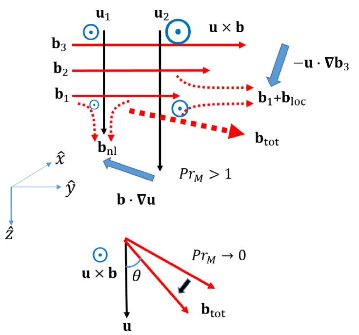


Dynamo process shown in Fig. 1 is mathematically straightforward. The interaction between and yields EMF (()), which is the weakest at & and strongest at & . This inhomogeneous EMF arouses a nontrivial curl effect, i.e., growth rate of magnetic field: . The growth rate is the weakest at & and strongest at & . This indicates energy transfer from () to (). Essentially the transport of magnetic energy occurs in a bimodal way. A transferred magnetic field from to through 111Here, a bold letter or indicates a vector field. is represented by (), which is parallel to the velocity field. Similarly, a transferred magnetic field from to through is represented by (), which is parallel to the magnetic field. Net magnetic field from these two transferred magnetic fields again interacts with at the next dynamo process.
In addition to the strength of and , the angle between and plays a crucial role in EMF. If grow faster than , and EMF decrease. Several factors can affect their relative ratio, but magnetic Prandtl number has a paradoxical effect. Both and are related to the dissipation of energy; but, their roles work in the opposite way. Decreasing increases and EMF. However, with small more kinetic energy is transported to a smaller eddy. Then, more magnetic energy is transferred to the smaller eddy leading to the growth of , which disturbs dynamo (see Fig. 6(a)).
In the model (or ) can be considered as a large or small scale field. However, as implies, if and are the small scale eddies, the magnetic energy transfer from () to () occurs more easily due to the small characteristic length. In contrast, if and are large scale eddies, additional process is required to overcome the large characteristic length . Nonetheless, the energy transport is essentially bidirectional, which appears clearly in a decaying MHD system (Park, 2017a, b).
2.1 Amplification of the helical field for LSD
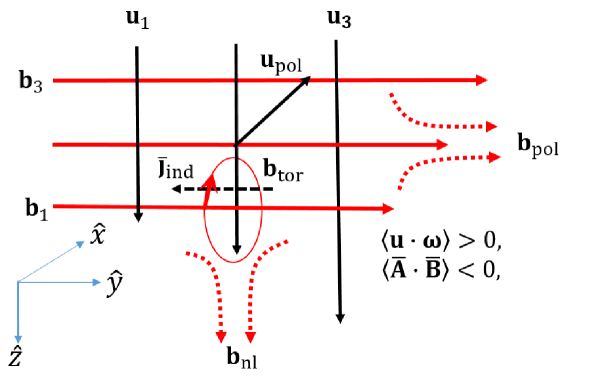
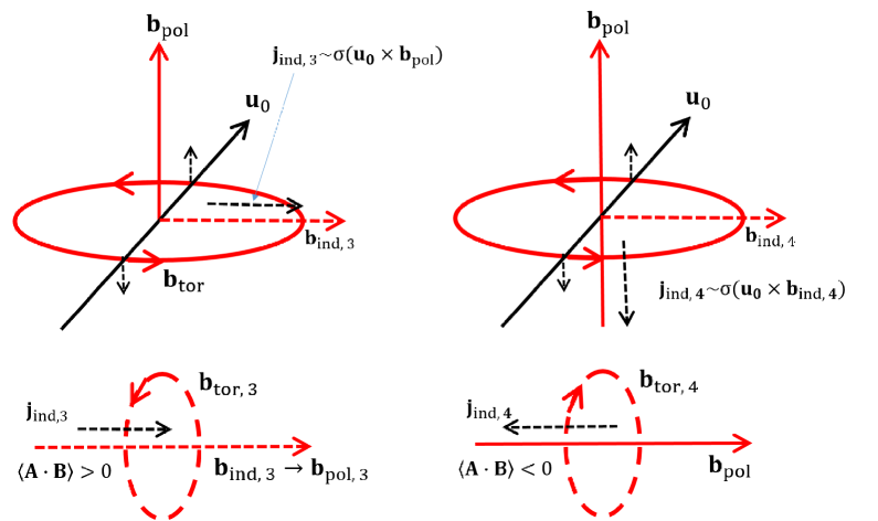
Fig. 2 shows a dynamo system forced by the right handed helical kinetic energy (HKF) composed of a toroidal field and poloidal one (. 222In Fig. 2 only a representative is considered to synchronize the two-scale dynamo theory. , , and the resultant left handed magnetic helicity exist in the whole scales. The interaction between and induces a current density , which generates a toroidal magnetic field around (=) forming a left handed magnetic helicity . interacts with to induce another circular current density antiparallel to . amplifies , which amplifies back through the dynamo process (Park, 2017a, b). This compound process makes possible surpasses and . As grows, dissipation effect plays a decisive role. So if is a small scale field, its dissipation () becomes larger than that of other eddies. Therefore should be a large scale field for the continuous dynamo process.
As increases, the energy diffuses toward through (Fig. 2). However, the direction of curl effect is opposite so the induced field heads for . can be inferred to approach to and regrow to be . Also, the toroidal field around is induced due to . The direction of does not change. Subsequently, and make the right handed magnetic helicity in small scale regime. This is supported by the changing sign of at minimum of (see Fig. 4). Simultaneously, can be suppressed by the interaction between and . Also, the growth of modifies the curvature radius of magnetic fields so that Lorentz force suppresses . All of these effects explain the conservation of magnetic helicity in HKFD.
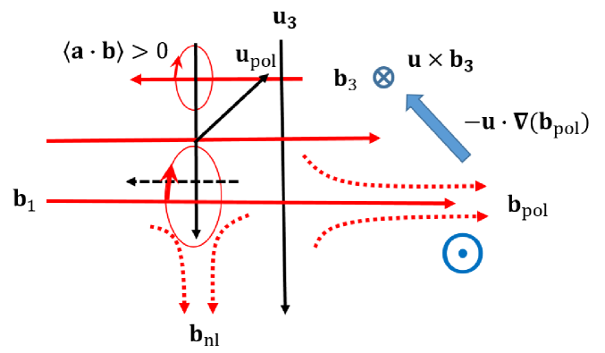
Left panel in Fig. 3(a) shows the dynamo process discussed above. However, right panel shows a different possibility that can generate which is parallel to the . induces , and forms the right handed magnetic helicity with . These two dynamo processes seem to result in net helicity. However, a careful look shows an essential difference between these two processes. The amplified due to the enhanced yields stronger , which amplifies . This toroidal field fortifies again, which produces the enhanced . In contrast, and do not have such a mutual interaction, rather evolve passively. This essential difference decides the dominant magnetic helicity in the system.
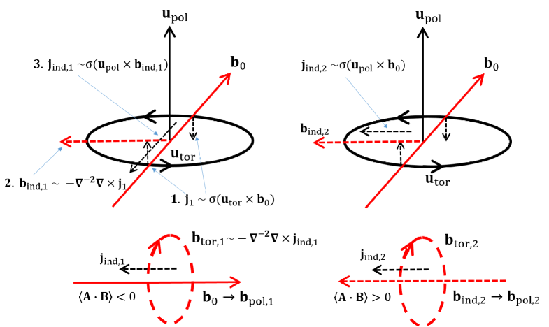
The principle of helical magnetic forcing dynamo (HMFD) in Fig. 3(b) is similar to that of HKFD except some slight but essential differences. In the system forced by the right handed (positive) helical magnetic energy, is generated from . But, can induce two different current densities: from and from . generates around leading to the right handed magnetic helicity. But, generates around to generate the left handed magnetic helicity. However, since is antiparallel to , the left handed magnetic helicity cancels with the injected right handed one. This is why the magnetic helicity generated in HMFD has the same sign of a forcing magnetic helicity.
2.2 Derivation of coefficients
Thus far, we have shown the physical mechanisms of LSD and SSD in the field structure. Being different from SSD, LSD requires an additional amplifying process of the field, effect. The model implies that the growth of field () is related to the (helical) motion of , in small scale and field itself. Therefore, if the characteristic length and time scale of turbulent eddies are smaller than those of , EMF may be expanded like:
| (4) |
Moreover, if a smaller quantity out of and is much smaller than ‘1’ (min), triple correlation terms and in the magnetic induction equation in the small scale regime can be neglected. Then, can be calculated from (Moffatt, 1978) or from (Keinigs, 1983). However, these anticommutative FOSAs are not generally valid besides the considerable in space. In MTA, the third order moment terms, neglected in FOSA, are replaced by without further calculation. It starts from the differentiation of a multi-variable function .
| (5) |
After some analytical calculations, we can derive the simple forms of and . Mathematically, the quenching effect of in the coefficient is from the definition of a vector product and differentiation of a multi variable function. Physically, it is caused by the interaction between the current density and magnetic field in different scales.
Additional differentiation of Eq. (5) produces the fourth order moments which can be decomposed into the combination of second order ones: (QN, Kraichnan & Nagarajan (1967)). With the assumption of isotropy without reflection symmetry, the second order moment can be replaced by
| (6) |
where , , and . With some calculations, , coefficient similar to those of MTA can be derived (Frisch et al., 1975).
All these methods are essentially to solve a closure issue in the MHD equations approximately without the exact solution of anisotropy and energy cascade time affected by the magnetic field. Therefore, if there is a practical method to find the exact , coefficient from observation and simulation, it will be helpful to infer a better closing method leading to a more exact helical dynamo theory.
2.3 Derivation of ‘’ and ‘’ coefficients using semi-analytic method
In principle, and coefficients can be found from . However, this vector equation is not so useful to the practical calculation. Instead, the scalar equations for and are more useful. We can get them like (Park, 2017b)
| (7) | |||||
| (8) |
The solutions of coupled Eqs. (7), (8) are333) includes the helical and nonhelical components of . However, the nonhelical component of is dropped when is averaged over the large scale.,
| (9) | |||||
| (10) | |||||
Eqs. (9), (10) are consistent with the field structure (Fig. 3(a), 3(b)) and the simulation results (Fig. 5(a), 5(b)). If (positive HKF or negative HMF), the second term in the right-hand side of Eqs. (9), (10) become dominant with increasing time. Since , becomes negative. In contrast, if (negative HKF or positive HMF), becomes positive and converges to eventually. But is positive in any case. When making these theoretical predictions, we referred to the simplest definitions of and coefficients. However, these coefficients can be derived from
| (11) | |||||
| (12) |
With and , we can further obtain the separate coefficients like
| (13) | |||||
| (14) |
As the results show, if we know the temporal changes of large scale magnetic helicity and large scale magnetic energy , and coefficients can be found. Considering that other theoretical and numerical methods to find these coefficients require considerable analytic calculations and elaborate simulations, which are not yet accurate, these results give us quite a clear method to find and coefficients. Additional differentiation over time leads to the integrand of each coefficients: , . They can give us a chance to test the classical analytic results of FOSA or MTA or . For a decaying MHD system, these classical results with Eq. (9), (10) reproduce the simulation results quite well (Park, 2017b). But still more numerical test is necessary for a forced system. There may be additional effects which are excluded in MTA and FOSA. Since the results Eq. (13), (14), which are mathematically derived with a statistical assumption and algebra, are exact as long as is valid, we will be able to see which other terms play a role in the effect.
3 Summary
Thus far, we have seen how the field structure model explains the amplification process of the magnetic field in the plasma. Magnetic field parallel to is transferred through , and magnetic field parallel to is transferred through . The net magnetic field from and is used as a seed magnetic field for the next dynamo step. As the field structure shows, growing parallel to suppresses the dynamo process, whereas growing perpendicular to boosts the dynamo action. This result explains the dependence of dynamo on the magnetic Prandtl number (). With less magnetic diffusion (decreasing ) and more kinetic dissipation (increasing , or increasing ), the dynamo effect elevates. In contrast, the decreasing mechanical dissipation decreases the dynamo effect. These relations imply that the saturation of the magnetic field in an ideal system is related to the field structure between and (angle ) rather than the dissipation effect. We also explained the mechanism of the helical dynamo ( effect) using vector field analysis. HKFD and HMFD can generate both of the positive and negative magnetic helicity in principle. However, as we discussed, only opposite (same) sign of magnetic helicity is left in a forced HKFD (HMFD) system. Finally, we derived , coefficients from the large-scale magnetic energy and magnetic helicity. The exact coefficients are useful to understanding more accurate internal dynamo processes in a MHD system, which leads to a more general dynamo theory. At present, the field structure model with various physical conditions such as rotation, shear, or remains to be done. Before doing that, we will test the method with the simulation results and observation data.
Acknowledgements
KWP appreciates the support from ERC Advanced Grant STARLIGHT: Formation of the First Stars (339177) and the support from bwForCluster for numerical simulation.
References
- Balbus & Hawley (1991) Balbus S. A., Hawley J. F., 1991, ApJ, 376, 214
- Blackman & Field (2002) Blackman E. G., Field G. B., 2002, Physical Review Letters, 89, 265007
- Brandenburg (2001) Brandenburg A., 2001, ApJ, 550, 824
- Brandenburg & Subramanian (2005) Brandenburg A., Subramanian K., 2005, Phys. Reports, 417, 1
- Cattaneo & Hughes (1996) Cattaneo F., Hughes D. W., 1996, Phys. Rev. E, 54, R4532
- Frisch et al. (1975) Frisch U., Pouquet A., Leorat J., Mazure A., 1975, Journal of Fluid Mechanics, 68, 769
- Keinigs (1983) Keinigs R. K., 1983, Physics of Fluids, 26, 2558
- Kraichnan & Nagarajan (1967) Kraichnan R. H., Nagarajan S., 1967, Physics of Fluids, 10, 859
- Krause & Rädler (1980) Krause F., Rädler K., 1980, Mean-field magnetohydrodynamics and dynamo theory
- Moffatt (1978) Moffatt H. K., 1978, Magnetic field generation in electrically conducting fluids
- Park (2017a) Park K., 2017a, Phys. Rev. D, 96, 083505
- Park (2017b) Park K., 2017b, Mon. Not. R. Astron. Soc., 472, 1628
- Park & Blackman (2012a) Park K., Blackman E. G., 2012a, MNRAS, 419, 913
- Park & Blackman (2012b) Park K., Blackman E. G., 2012b, MNRAS, 423, 2120
- Rogachevskii & Kleeorin (2003) Rogachevskii I., Kleeorin N., 2003, Phys. Rev. E, 68, 036301
- Schekochihin et al. (2002) Schekochihin A. A., Maron J. L., Cowley S. C., McWilliams J. C., 2002, ApJ, 576, 806
- Schrinner et al. (2005) Schrinner M., Rädler K.-H., Schmitt D., Rheinhardt M., Christensen U., 2005, Astronomische Nachrichten, 326, 245
- Zeldovich (1983) Zeldovich Y. B., 1983, Magnetic fields in astrophysics