Private Information Retrieval From a Cellular Network With Caching at the Edge
Abstract
We consider the problem of downloading content from a cellular network where content is cached at the wireless edge while achieving privacy. In particular, we consider private information retrieval (PIR) of content from a library of files, i.e., the user wishes to download a file and does not want the network to learn any information about which file she is interested in. To reduce the backhaul usage, content is cached at the wireless edge in a number of small-cell base stations using maximum distance separable codes. We propose a PIR scheme for this scenario that achieves privacy against a number of spy SBSs that (possibly) collaborate. The proposed PIR scheme is an extension of a recently introduced scheme by Kumar et al. to the case of multiple code rates, suitable for the scenario where files have different popularities. We then derive the backhaul rate and optimize the content placement to minimize it. We prove that uniform content placement is optimal, i.e., all files that are cached should be stored using the same code rate. This is in contrast to the case where no PIR is required. Furthermore, we show numerically that popular content placement is optimal for some scenarios.
I Introduction
Bringing content closer to the end user in wireless networks, the so-called caching at the wireless edge, has emerged as a promising technique to reduce the backhaul usage. The literature on wireless caching is vast. Information-theoretic aspects of caching were studied in [1, 2]. To leverage the potential gains of caching, several papers proposed to cache files in densely deployed small-cell base stations (SBSs) with large storage capacity, see, e.g., [3, 4, 5, 6, 7]. In [5], content is cached in SBSs using maximum distance separable (MDS) codes to reduce the download delay. This scenario was further studied in [7], where the authors optimized the MDS-coded caching to minimize the backhaul rate. Caching content directly in the mobile devices and exploiting device-to-device communication has been considered in, e.g., [8, 9, 10, 11, 12].
Recently, private information retrieval (PIR) has attracted a significant interest in the research community [13, 14, 15, 16, 17, 18, 19, 20, 21, 22, 23]. In PIR, a user would like to retrieve data from a distributed storage system (DSS) in the presence of spy nodes, without revealing any information about the piece of data she is interested in to the spy nodes. PIR was first studied by Chor et al. [24] for the case where a binary database is replicated among servers (nodes) and the aim is to privately retrieve a single bit from the database in the presence of a single spy node (referred to as the noncolluding case), while minimizing the total communication cost. In the last few years, spurred by the rise of DSSs, research on PIR has been focusing on the more general case where data is stored using a storage code.
The PIR capacity, i.e., the maximum achievable PIR rate, was studied in [18, 19, 21, 22, 23]. In [19, 23], the PIR capacity was derived for the scenario where data is stored in a DSS using a repetition code. In [22], for the noncolluding case, the authors derived the PIR capacity for the scenario where data is stored using an (single) MDS code, referred to as the MDS-PIR capacity. For the case where several spy nodes collaborate with each other, referred to as the colluding case, the MDS-PIR capacity is in general still unknown, except for some special cases [18] (and for repetition codes [23]). PIR protocols for DSSs have been proposed in [14, 16, 17, 20, 21]. In [16], a PIR protocol for MDS-coded DSSs was proposed and shown to achieve the MDS-PIR capacity for the case of noncolluding nodes when the number of files stored in the DSS goes to infinity. PIR protocols for the case where data is stored using non-MDS codes were proposed in [17, 20, 21].
In this paper, we consider PIR of content from a cellular network. In particular, we consider the private retrieval of content from a library of files that have different popularities. We consider a similar scenario as in [7] where, to reduce the backhaul usage, content is cached in SBSs using MDS codes. We propose a PIR scheme for this scenario that achieves privacy against a number of spy SBSs that possibly collude. The proposed PIR scheme is an extension of Protocol 3 in [21] to the case of multiple code rates, suitable for the scenario where files have different popularities. We also propose an MDS-coded content placement slightly different than the one in [7] but that is more adapted to the PIR case. We show that, for the conventional content retrieval scenario with no privacy, the proposed content placement is equivalent to the one in [7], in the sense that it yields the same average backhaul rate. We then derive the backhaul rate for the PIR case as a function of the content placement. We prove that uniform content placement, i.e., all files that are cached are encoded with the same code rate, is optimal. This is a somewhat surprising result, in contrast to the case where no PIR is considered, where optimal content placement is far from uniform [7]. We further consider the minimization of a weighted sum of the backhaul rate and the communication rate from the SBSs, relevant for the case where limiting the communication from the SBSs is also important. We finally report numerical results for both the scenario where SBSs are placed regularly in a grid and for a Poisson point process (PPP) deployment model where SBSs are distributed over the plane according to a PPP. We show numerically that popular content placement is optimal for some system parameters. To the best of our knowledge, PIR for the wireless caching scenario has not been considered before.
Notation: We use lower case bold letters to denote vectors, upper case bold letters to denote matrices, and calligraphic upper case letters to denote sets. For example, , , and denote a vector, a matrix, and a set, respectively. We denote a submatrix of that is restricted in columns by the set by . will denote a linear code over the finite field . The multiplicative subgroup of (not containing the zero element) is denoted by . We use the customary code parameters to denote a code of blocklength and dimension . A generator matrix for will be denoted by and a parity-check matrix by . A set of coordinates of , , of size is said to be an information set if and only if is invertible. The Hadamard product of two linear subspaces and , denoted by , is the space generated by the Hadamard products for all pairs , . The inner product of two vectors and is denoted by , while denotes the Hamming weight of . represents the transpose of its argument, while represents the entropy function. With some abuse of language, we sometimes interchangeably refer to binary vectors as erasure patterns under the implicit assumption that the ones represent erasures. An erasure pattern (or binary vector) is said to be correctable by a code if matrix has rank .
II System Model
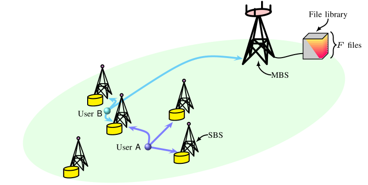
We consider a cellular network where a macro-cell is served by a macro base station (MBS). Mobile users wish to download files from a library of files that is always available at the MBS through a backhaul link. We assume all files of equal size.111Assuming files of equal size is without loss of generality, since content can always be divided into chunks of equal size. In particular, each file consists of bits and is represented by a matrix ,
where upperindex is the file index. Therefore, each file can be seen as divided into stripes of bits each. The file library has popularity distribution , where file is requested with probability . We also assume that SBSs are deployed to serve requests and offload traffic from the MBS whenever possible. To this purpose, each SBS has a cache size equivalent to files. The considered scenario is depicted in Fig. 1.
II-A Content Placement
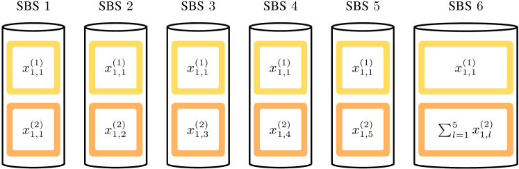
File is partitioned into packets of size bits and encoded before being cached in the SBSs. In particular, each packet is mapped onto a symbol of the field , with . For simplicity, we assume that is integer and set . Thus, stripe can be equivalently represented by a stripe , , of symbols over . Each stripe is then encoded using an MDS code over into a codeword , where code symbols , , are over . For later use, we define , , and .
The encoded file can be represented by a matrix . Code symbols are then stored in the -th SBS (the ordering is unimportant). Thus, for each file , each SBS caches one coded symbol of each stripe of the file, i.e., a fraction of the -th file. As ,
where implies that file is not cached. Note that, to achieve privacy, , i.e., files need to be cached with redundancy. As a result, is not allowed. This is in contrast to the case of no PIR, where (and hence ) is possible.
Since each SBS can cache the equivalent of files, the ’s must satisfy
We define the vector and refer to it as the content placement. Also, we denote by the caching scheme that uses MDS codes according to the content placement . For later use, we define and .
We remark that the content placement above is slightly different than the content placement proposed in [7]. In particular, we assume fixed code length (equal to the number of SBSs, ) and variable , such that, for each file cached, each SBS caches a single symbol from each stripe of the file. In [7], the content placement is done by first dividing each file into symbols and encoding them using an MDS code, where , . Then, (different) symbols of the -th file are stored in each SBS and the MBS stores symbols.222This is because the model in [7] assumes that one SBS is always accessible to the user. If this is not the case, the MBS must store all symbols of the file. Here, we consider the case where the MBS must store all symbols because it is a bit more general. Our formulation is perhaps a bit simpler and more natural from a coding perspective. Furthermore, we will show in Section IV that the proposed content placement is equivalent to the one in [7], in the sense that it yields the same average backhaul rate.
II-B File Request
Mobile devices request files according to the popularity distribution . Without loss of generality, we assume . The user request is initially served by the SBSs within communication range. We denote by the probability that the user is served by SBSs and define . If the user is not able to completely retrieve from the SBSs, the additional required symbols are fetched from the MBS. Using the terminology in [7], the average fraction of files that are downloaded from the MBS is referred to as the backhaul rate, denoted by R, and defined as
Note that for the case of no caching .
As in [7], we assume that the communication is error free.
II-C Private Information Retrieval and Problem Formulation
We assume that some of the SBSs are spy nodes that (potentially) collaborate with each other. On the other hand, we assume that the MBS can be trusted. The users wish to retrieve files from the cellular network, but do not want the spy nodes to learn any information about which file is requested by the user. The goal is to retrieve data from the network privately while minimizing the use of the backhaul link, i.e., while minimizing R. Thus, the goal is to optimize the content placement to minimize R.
III Private Information Retrieval Protocol
In this section, we present a PIR protocol for the caching scenario. The PIR protocol proposed here is an extension of Protocol 3 in [21] to the case of multiple code rates.333Protocol 3 in [21] is based on and improves the protocol in [20], in the sense that it achieves higher PIR rates.
Assume without loss of generality that the user wants to download file . To retrieve the file, the user generates query matrices, , , where are the queries sent to the SBSs within visibility and the remaining queries are sent to the MBS. Note that is a parameter that needs to be optimized. Each query matrix is of size symbols (from ) and has the following structure,
The query matrix consists of subqueries , , of length symbols each. In response to query matrix , a SBS (or the MBS) sends back to the user a response vector of length , computed as
| (1) |
We will denote the -th entry of the response vector , i.e., , as the -th subresponse of . Each response vector consists of subresponses, each being a linear combination of symbols. Note that the operations are performed over the largest extension field, i.e., , and the subresponses are also over this field, i.e., each subresponse is of size bits and hence each response is of size bits.
The queries and the responses must be such that privacy is ensured and the user is able to recover the requested file. More precisely, information-theoretic PIR in the context of wireless caching with spy SBSs is defined as follows.
Definition 1.
Consider a wireless caching scenario with SBSs that cache parts of a library of files and in which a set of SBSs act as colluding spies. A user wishes to retrieve the -th file and generates queries , . In response to the queries the SBSs and (potentially) the MBS send back the responses . This scheme achieves perfect information-theoretic PIR if and only if
| Privacy: | (2a) | |||
| Recovery: | (2b) | |||
Condition (2a) means that the spy SBSs gain no additional information about which file is requested from the queries (i.e., the uncertainty about the file requested after observing the queries is identical to the a priori uncertainty determined by the popularity distribution), while Condition (2b) guarantees that the user is able to recover the file from the response vectors.
We define the code , , as the code obtained by puncturing the underlying storage code , and by the code with parameters .444Without loss of generality, to simplify notation we assume that the last coordinates of the code are puntured. For the protocol to work, we require that divides for all , i.e., . This ensures that . Furthermore, we require the codes to be such that . The protocol is characterized by the codes and by two other codes, and . Code (over ) has parameters and characterizes the queries sent to the SBSs and the MBS, while code (defined below) defines the responses sent back to the user from the SBSs and the MBS. The designed protocol achieves PIR against a number of colluding SBSs , where is the minimum Hamming distance of the dual code of .
III-A Query Construction
The queries must be constructed such that privacy is preserved and the user can retrieve the requested file from the response vectors , . In particular, the protocol is designed such that the subresponses , , corresponding to the subqueries recover unique code symbols of the file .
The queries are constructed as follows. The user chooses codewords , , , independently and uniformly at random. Then, the user constructs vectors,
| (3) |
where collects the -th coordinates of the codewords , , i.e., .
Assume that the user wants to retrieve file . Then, subquery is constructed as
| (4) |
where
| (5) |
for some set that will be defined below. Vector , , denotes the -th -dimensional unit vector, i.e., the length- vector with a one in the -th coordinate and zeroes in all other coordinates, and the all-zero vector. The meaning of index will become apparent later.
According to (4), each subquery vector is the sum of two vectors, and . The purpose of is to make the subquery appear random and thus ensure privacy (i.e., Condition (2a)). On the other hand, the vectors are deterministic vectors which must be properly constructed such that the user is able to retrieve the requested file from the response vectors (i.e., Condition (2b)). Similar to Protocol 3 in [21], the vectors are constructed from a binary matrix where each row represents a weight- erasure pattern that is correctable by and where the weights of its columns are determined from information sets , , of .
The construction of is addressed below. We define the set as the index set of information sets that contain the -th coordinate of , i.e., . To allow the user to recover the requested file from the response vectors, is constructed such that it satisfies the following conditions.
-
The user should be able to recover unique code symbols of the requested file from the responses to each set of subqueries , . This is to say that each row of should have exactly ones. We denote by the support of the -th row of .
-
The user should be able to recover unique code symbols of the requested file , at least symbols from each stripe. This means that each row , , of should correspond to an erasure pattern that is correctable by .
-
Let , , be the -th column vector of . The protocol should be able to recover unique code symbols from the -th response vector, which means that it is required that . We call the vector the column weight profile of .
III-B Response Vectors
The -th subresponse corresponding to subquery , , is (see (1))
The user collects the subresponses , , in the vector ,
| (6) |
where symbol represents the code symbol from file downloaded in the -th subresponse from the -th response vector. Due to the structure of the queries obtained from , the user retrieves code symbols from the set of subresponses to the -th subqueries. Consider a retrieval code of the form
| (7) |
where denotes the sum of subspaces and , resulting in the set consisting of all elements for any and , and where follows due to the fact that the Hadamard product is distributive over addition.
The symbols requested by the user are then obtained solving the system of linear equations defined by
III-C Privacy
For the retrieval, we require to be a valid code, i.e., it must have a code rate strictly less than . For a given number of colluding SBSs , the combination of conditions on and restricts the choice for the underlying storage codes . In the following theorem, we present a family of MDS codes, namely generalized Reed-Solomon (GRS) codes, that work with the protocol. A GRS code over of length and dimension is a weighted polynomial evaluation code of degree defined by some weighting vector and an evaluation vector satisfying for all [25, Ch. 5]. In the sequel, we refer to as the parameters of a GRS code .
Lemma 1.
Given an GRS code , for all , there exists an GRS code that is a subcode of .
Proof:
The canonical generator matrix for an GRS code is given by
| (8) |
Clearly, taking the first rows of the leftmost matrix of (8) and multiplying it with the rightmost diagonal matrix generates an subcode of which by itself is an GRS code. Thus, GRS codes are naturally nested, and the result follows. ∎
Theorem 1.
Let be a caching scheme with GRS codes of parameters and let be the code obtained by puncturing . Also, let be an GRS code. Then, for and , the protocol achieves PIR against colluding SBSs.
Proof:
The proof is given in the appendix. ∎
Note that the retrieval code depends on the SBSs within visibility that are contacted by the user through its evaluation vector. Finally, we remark that, with some slight modifications, the proposed protocol can be adapted to work with non-MDS codes.
III-D Example
As an example, consider the case of files, and , both of size bits. The first file is stored in the SBSs according to Fig. 2 using an binary repetition code . Similarly, the second file is stored (again according to Fig. 2) using an binary single parity-check code . Assume (i.e., no puncturing) and that none of the SBSs collude, i.e., . Furthermore, we assume that the user wants to retrieve and is able to contact SBSs (i.e., we consider the extreme case where the user is not contacting the MBS). According to Theorem 1, we can choose and . Finally, we choose as an binary repetition code.
According to (7), the retrieval code and can be generated by
Moreover, let
where is an information set of (the submatrix has rank ). Note that satisfies all three conditions – and has column weight profile .
Query Construction. The user generates codewords and independently and uniformly at random from . Without loss of generality, let . Next, the subqueries , , are constructed according to 4, 5 as
where is defined in (3).
File Retrieval. Consider the subresponses , . Then, according to (III-B),
and the code symbol of the file is recovered from
Note that in order to retain privacy across the two files of the library, we need to send subqueries to each SBS, thus generating subresponses from each SBS (even if the first file can be recovered from the subresponses , ).
IV Backhaul Rate Analysis: No PIR Case
In this section, we derive the backhaul rate for the proposed caching scheme for the case of no PIR, i.e., the conventional caching scenario where PIR is not required.
Proposition 1.
The average backhaul rate for the caching scheme in Section II for the case of no PIR is
| (9) |
Proof:
To download file , if the user is in communication range of a number of SBSs, , larger than or equal to , the user can retrieve the file from the SBSs and there is no contribution to the backhaul rate. Otherwise, if , the user retrieves a fraction of the file from each of the SBSs, i.e., a total of bits, and downloads the remaining bits from the MBS. Averaging over and (for the files cached) and normalizing by the file size , the contribution to the backhaul rate of the retrieval of files that are cached in the SBSs is
| (10) |
On the other hand, the files that are not cached are retrieved completely from the MBS, and their contribution to the backhaul rate is
| (11) |
We denote by the maximum PIR rate resulting from the optimization of the content placement. can be obtained solving the following optimization problem,
where , as is a valid value for the case where PIR is not required.
In the following lemma, we show that the proposed content placement is equivalent to the one in [7], in the sense that it yields the same average backhaul rate.
Lemma 2.
Proof:
For popular content placement, i.e., the case where the most popular files are cached in all SBSs (this corresponds to caching the most popular files using an repetition code, i.e., for and for ), the backhaul rate is given by
| (12) |
V Backhaul Rate Analysis: PIR Case
In this section, we derive the backhaul rate for the case of PIR (i.e., when the user wishes to download content privately) and we prove that uniform content placement (under the PIR protocol in Section III with GRS codes) is optimal. The average backhaul rate is given in the following proposition.
Proposition 2.
The average backhaul rate for the caching scheme in Section II (with GRS codes) for the PIR case is
| (13) |
Proof:
To download file , the user generates query matrices. If the user is in communication range of SBSs, it receives responses (one from each SBS). The responses to the remaining query matrices need to be downloaded from the MBS. Since each response consists of subresponses of size bits, the user downloads bits from the MBS. Averaging over and (for the files cached) and normalizing by the file size , the contribution to the backhaul rate of the retrieval of files that are cached in the SBSs is
| (14) |
Now, using the fact that and (see Theorem 1), we can rewrite (14) as
| (15) |
V-A Optimal Content Placement
Let be the maximum PIR rate resulting from the optimization of the content placement. can be obtained solving the following optimization problem,
| (17) | ||||
where and the minimum value that can take on, i.e., , comes from the fact that has to be positive.
Lemma 3.
Uniform content allocation, i.e., for all files that are cached, is optimal. Furthermore, the optimal number of files to cache is the maximum possible, i.e., for .
Proof:
We first prove the first part of the lemma. We need to show that either the optimal solution to the optimization problem in (V-A) is the all-zero vector , or there exists a nonzero optimal solution for which . Consider the second case, and let denote any nonzero feasible solution to (V-A), i.e., a nonzero solution that satisfies the cache size constraint. Furthermore, let denote the length- vector obtained from as for and otherwise. Clearly, satisfies the cache size constraint as well. Note that . Thus,
Furthermore, since both the double summation in the first term of the objective function in (V-A) and the second term in (V-A) only depend on the support of , it follows that the value of the objective function for is smaller than or equal to the value of the objective function for . Thus, for any nonzero feasible solution there exists another at least as good nonzero feasible solution for which all nonzero entries are the same (i.e., ), and the result follows by applying the above procedure to a (nonzero) optimal solution to (V-A).
We now prove the second part of the lemma. Caching a file helps in reducing the backhaul rate if
| (18) |
for some and . This is independent of the file index . Thus, if the optimal solution is to cache at least one file (), (18) is met for some and caching other files (as many files as permitted up to the cache size constraint, with decreasing order of popularity) is optimal as it further reduces the backhaul rate. ∎
V-B Popular Content Placement
For popular content placement, the backhaul rate is given by
| (20) |
Note that the optimization over is still required.
VI Weighted Communication Rate
So far, we have considered only the backhaul rate. However, it might also be desirable to limit the communication rate from SBSs to the user. We thus consider the weighted communication rate, , defined as555For the case of no PIR, a linear scalarization of the MBS and SBS download delays was considered in [5]. The communication rate is directly related to the download delay.
where is the average communication rate (normalized by the file size ) from the SBSs, and is a weighting parameter. We consider , stemming from the fact that the bottleneck is the backhaul. Note that minimizing the average backhaul rate corresponds to .
Proposition 3.
The average communication rate from the SBSs for the caching scheme in Section II (with GRS codes) for the PIR case is
| (21) |
where for and .
Proof:
To ensure privacy, the user needs to download data from the SBSs within visibility regardless whether the requested file is cached or not. This is in contrast to the case of no PIR. Note that, if the user queries the SBSs only in the case the requested file is cached, then the spy SBSs would infer that the user is interested in one of the files cached, thus gaining some information about the file requested. In other words, the user sends dummy queries and downloads data that is useless for the retrieval of the file but is necessary to achieve privacy. The user receives responses from the SBSs within communication range, each of size bits. Let denote the probability to receive responses from SBSs. For , is equal to the probability that SBSs are within communication range, i.e., . On the other hand, the probability to receive responses from SBSs, , is the probability that at least SBSs are within communication range, i.e., . Averaging over and (for all files, cached and not cached) and normalizing by the file size , the contribution to the communication rate of the retrieval of a file from the SBSs is
| (22) |
Now, using the fact that and (see Theorem 1), we can rewrite (22) as (21). ∎
Lemma 4.
Uniform content allocation, i.e., for all files that are cached, is optimal. Furthermore, the optimal number of files to cache is the maximum possible, i.e., for .
VII Numerical Results
For the numerical results in this section, we assume that the files popularity distribution follows the Zipf law [26], i.e., the popularity of file is
where is the skewness factor [7] and by definition . In Figs. 3 and 4, we consider a network topology where SBSs are deployed over a macro-cell of radius meters according to a regular grid with distance meters between them [7, 5]. Each SBS has a communication radius of meters. Let be the area where a user can be served by SBSs. Then, assuming that the users are uniformly distributed over the macro-cell area with density users per square meter, the probability that a user is in communication range of SBSs can be calculated as in [7]
where the areas can be easily obtained by simple geometrical evaluations, and is the maximum number of SBSs within communication range of a user.
For the results in Figs. 3 and 4, the system parameters (taken from [7]) are meters, which results in over the macro-cell area, files, , and meters. This results in , i.e., the maximum number of SBSs in visibility of a user is .
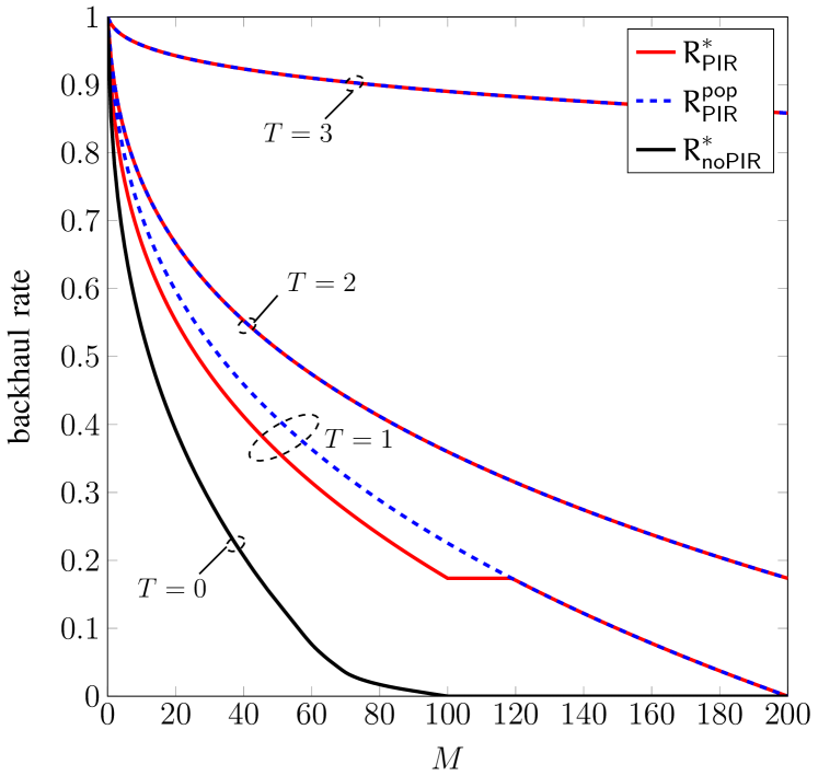
In Fig. 3, we plot the optimized backhaul rate (red, solid lines) according to (19) as a function of the cache size constraint for the noncolluding case () and and colluding SBSs. The curves in Fig. 3 should be interpreted as the minimum backhaul rate that is necessary in order to achieve privacy against spy SBSs out of the SBSs that are contacted by the user. For the particular system parameters considered, the optimal value of is for and , and all values of , i.e., the scheme yields privacy against spy SBSs out of the SBSs contacted. For the optimal value of is for all values of , and thus the scheme yields privacy against spy SBSs out of SBSs. We also plot the optimized backhaul rate for the case of no PIR.666The curve in the figure is identical to that in [7, Fig. 4]. As proved in Lemma 2, while the proposed content placement is different from the one in [7], they are equivalent in terms of average backhaul rate. As can be seen in the figure, caching helps in significantly reducing the backhaul rate for and . For caching also helps in reducing the backhaul rate, but the reduction is smaller. Also, as expected, compared to the case of no PIR (, black, solid line) achieving privacy requires a higher backhaul rate. The required backhaul rate increases with the number of colluding SBSs .
For and no PIR, the backhaul rate is zero, as all files can be downloaded from the SBSs. Indeed, for , we can select and cache one coded symbol from each stripe of each file in each SBS (thus satisfying the constraint as ). Since for no PIR to retrieve each stripe of a file it is enough to download symbols from each stripe of the file (due to the MDS property) and according to at least SBSs are within range, for (and hence for as well) the user can always retrieve the file from the SBSs and the backhaul rate is zero. For the case of PIR and , on the other hand, the required backhaul rate is positive unless all complete files can be cached in all SBSs, i.e., . For and , even for the backhaul rate is not zero. This is because in this case the user needs to receive and responses , , respectively (from the SBSs or the MBS). However, for the considered system parameters the probability that the user has SBSs within range is not one, thus the user always needs to download data from the MBS to recover the file and the backhaul rate is positive.
For comparison purposes, in the figure we also plot the backhaul rate for the case of popular content placement in (20) (blue, dashed lines). In this case, the optimal value of is , , and for , , and , respectively. We remark that the curve for overlaps with the curve . This is due to the fact that for , , and , in (20) boils down to , which is in (12). However, for the general case, i.e., other , and may differ. As already shown in [7], for no PIR the optimized content placement yields significantly lower backhaul rate than popular content placement. For the PIR case and , up to the optimized content placement also yields some performance gains with respect to popular content placement, albeit not as significant as for the case of no PIR. Interestingly, as shown in the figure, for , PIR popular content placement is optimal. Furthermore, as shown in the figure, for and popular content placement is optimal for all .
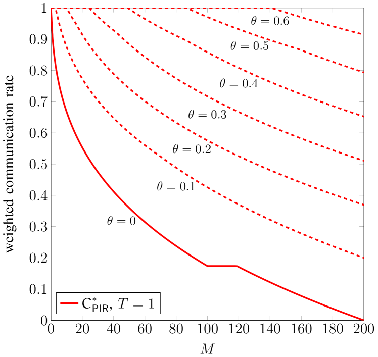
In Fig. 4, we plot the optimized weighted communication rate in (24) for the noncolluding case () as a function of the cache size constraint and several values of . For the considered system parameters, caching is still useful for small values of if the cache size is big enough. For example, for caching helps in reducing the weighted communication rate with respect to no caching for . For , caching does not bring any reduction of the weighted communication rate.
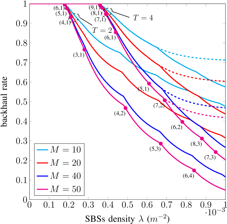
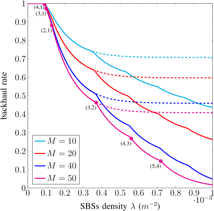
In Figs. 5 and 6, we plot the backhaul rate for a PPP deployment model where SBSs are distributed over the plane according to a PPP and a user at an arbitrary location in the plane can connect to all SBSs that are within radius . Let be the density of SBSs per square meter. For this scenario, the probability that a user is in communication range of SBSs is given by [27]
where . In Fig. 5, we plot the optimized backhaul rate ( in (19), solid lines) as a function of the density for files, , meters, different cache size constraint , and a single spy SBS, i.e., . For small densities, caching does not help in reducing the backhaul rate. However, as expected, the required backhaul rate diminishes by increasing the density of SBSs. For comparison purposes, we also plot the backhaul rate for popular content placement ( in (20), dashed lines). Interestingly, popular content placement is optimal up to a given density of SBSs, after which optimizing the content placement brings a significant reduction of the required backhaul rate. Similar results are observed for and colluding SBSs in Fig. 6 with the same system parameters as in Fig. 5. In Figs. 5 and 6, for each the optimal value of and depends on the density of SBSs. Typically, a pair is optimal for a range of densities. In the figures, we give the optimal values of and for (in particular we give the pair , with , which is also the code parameters of the punctured code ). For convenience, in the figures we only give the parameters for the densities where the optimal pair changes. The values should be read as follows: In Fig. 5, walking the curve from top-left to bottom-right, no caching is optimal for densities up to . For , is optimal. Then, is optimal for densities to . From to the optimal value is , and so on (the curves are plotted with steps of ).
VIII Conclusion
We proposed a private information retrieval scheme that allows to download files of different popularities from a cellular network, where to reduce the backhaul usage content is cached at the wireless edge in SBSs, while achieving privacy against a number of spy SBSs. We derived the backhaul rate for this scheme and formulated the content placement optimization. We showed that, as for the no PIR case, up to a number of spy SBSs caching helps in reducing the backhaul rate. Interestingly, contrary to the no PIR case, uniform content placement is optimal. Furthermore, popular content placement is optimal for some scenarios. Although uniform content placement is optimal, the proposed PIR scheme for multiple code rates may be useful in other scenarios, e.g., for distributed storage where data is stored using codes of different rates.
Appendix
Proof of Theorem 1
To prove that the protocol achieves PIR against colluding SBSs, we need to prove that both the privacy condition in (2a) and the recovery condition in (2b) are satisfied. We first prove that the recovery condition in (2b) is satisfied.
According to Lemma 1, GRS codes with a fixed weighting vector and evaluation vector are naturally nested. Furthermore, puncturing a GRS code results in another GRS code, since GRS codes are weighted evaluation codes [25, Ch. 5]. Thus, for all , and it follows from 7 that
Furthermore, it can easily be shown that the Hadamard product of two GRS codes with the same evaluation vector is also a GRS code with dimension equal to the sum of the dimensions minus . Thus, is a GRS code of dimension . As is an MDS code (GRS codes are MDS codes), it can correct arbitrary erasure patterns of up to erasures. This implies that one can construct a valid () matrix (satisfying conditions –) from information sets of as shown below.
Let , . Construct in such a way that is the support of the -th row of . Hence, is satisfied. Furthermore, since is an MDS code and , all rows of are correctable by , and thus is satisfied. Finally, run Algorithm 1, which constructs information sets of (and the corresponding sets ) such that is satisfied. Note that since is an MDS code, all coordinate sets of size are information sets of , and hence Algorithm 1 will always succeed in constructing a valid set of information sets of (the inequalities in Algorithms 1 and 1 together with the fact that the overall weight of is ensure that valid information sets for are constructed). In particular, the while-loop in Algorithm 1 will always terminate.
From the constructed matrix , the user is able to recover unique code symbols of the requested file , at least symbols from each stripe. Furthermore, a set of recovered code symbols from each stripe corresponds to an information set of (any subset of size of any information set of size of is an information set of ), and the requested file can be recovered. This can be seen following a similar argument as in the proof of [21, Th. 6], and it follows that the recovery condition in (2b) is satisfied.
Secondly, we consider the privacy condition in (2a). A reasoning similar to the proof of [21, Lem. 6] shows that it is satisfied, and we refer the interested reader to this proof for further details. The fundamental reason is that addition of a deterministic vector in (5) does not change the joint probability distribution of for any set size , and the proof follows the same lines as the proof of [20, Th. 8]. However, note that there is a subtle difference in the sense that independent instances of the protocol may query different sets of SBSs. However, since the set of SBSs that are queried is independent of the requested file and depends only on which SBSs that are within communication range, this fact does not leak any additional information on which file is requested by the user.
References
- [1] U. Niesen, D. Shah, and G. W. Wornell, “Caching in wireless networks,” IEEE Trans. Inf. Theory, vol. 58, no. 10, pp. 6524–6540, Oct. 2012.
- [2] M. A. Maddah-Ali and U. Niesen, “Fundamental limits of caching,” IEEE Trans. Inf. Theory, vol. 60, no. 5, pp. 2856–2867, May 2014.
- [3] J. G. Andrews, S. Buzzi, W. Choi, S. V. Hanly, A. Lozano, A. C. K. Soong, and J. C. Zhang, “What will 5G be?” IEEE J. Sel. Areas Commun., vol. 32, no. 6, pp. 1065–1082, Jun. 2014.
- [4] D. Liu, B. Chen, C. Yang, and A. F. Molisch, “Caching at the wireless edge: Design aspects, challenges, and future directions,” IEEE Commun. Mag., vol. 54, no. 9, pp. 22–28, Sep. 2016.
- [5] K. Shanmugam, N. Golrezaei, A. G. Dimakis, A. F. Molisch, and G. Caire, “Femtocaching: Wireless content delivery through distributed caching helpers,” IEEE Trans. Inf. Theory, vol. 59, no. 12, pp. 8402–8413, Dec. 2013.
- [6] E. Bastug, M. Bennis, and M. Debbah, “Living on the edge: The role of proactive caching in 5G wireless networks,” IEEE Commun. Mag., vol. 52, no. 8, pp. 82–89, Aug. 2014.
- [7] V. Bioglio, F. Gabry, and I. Land, “Optimizing MDS codes for caching at the edge,” in Proc. Global Commun. Conf. (GLOBECOM), San Diego, CA, Dec. 2015.
- [8] M. Ji, G. Caire, and A. F. Molisch, “Fundamental limits of caching in wireless D2D networks,” IEEE Trans. Inf. Theory, vol. 62, no. 2, pp. 849–869, Feb. 2016.
- [9] N. Golrezaei, P. Mansourifard, A. F. Molisch, and A. G. Dimakis, “Base-station assisted device-to-device communications for high-throughput wireless video networks,” IEEE Trans. Wireless Commun., vol. 13, no. 7, pp. 3665–3676, Jul. 2014.
- [10] J. Pedersen, A. Graell i Amat, I. Andriyanova, and F. Brännström, “Distributed storage in mobile wireless networks with device-to-device communication,” IEEE Trans. Commun., vol. 64, no. 11, pp. 4862–4878, Nov. 2016.
- [11] A. Piemontese and A. Graell i Amat, “MDS-coded distributed storage for low delay wireless content delivery,” in Proc. 2016 9th Int. Symp. Turbo Codes & Iterative Inform. Process. (ISTC), Brest, France, 2016, pp. 320–324.
- [12] J. Pedersen, A. Graell i Amat, I. Andriyanova, and F. Brännström, “Optimizing MDS coded caching in wireless networks with device-to-device communication,” Jan. 2017, arXiv:1701.06289v2 [cs.IT]. [Online]. Available: https://arxiv.org/abs/1701.06289
- [13] Y. Ishai, E. Kushilevitz, R. Ostrovsky, and A. Sahai, “Batch codes and their applications,” in Proc. 36th Annual ACM Symp. Theory Comput. (STOC), Chicago, IL, Jun. 2004, pp. 262–271.
- [14] N. B. Shah, K. V. Rashmi, and K. Ramchandran, “One extra bit of download ensures perfectly private information retrieval,” in Proc. IEEE Int. Symp. Inf. Theory (ISIT), Honolulu, HI, Jun./Jul. 2014, pp. 856–860.
- [15] T. H. Chan, S.-W. Ho, and H. Yamamoto, “Private information retrieval for coded storage,” in Proc. IEEE Int. Symp. Inf. Theory (ISIT), Hong Kong, China, Jun. 2015, pp. 2842–2846.
- [16] R. Tajeddine and S. El Rouayheb, “Private information retrieval from MDS coded data in distributed storage systems,” in Proc. IEEE Int. Symp. Inf. Theory (ISIT), Barcelona, Spain, Jul. 2016, pp. 1411–1415.
- [17] S. Kumar, E. Rosnes, and A. Graell i Amat, “Private information retrieval in distributed storage systems using an arbitrary linear code,” in Proc. IEEE Int. Symp. Inf. Theory (ISIT), Aachen, Germany, Jun. 2017, pp. 1421–1425.
- [18] H. Sun and S. A. Jafar, “Private information retrieval from MDS coded data with colluding servers: Settling a conjecture by Freij-Hollanti et al.” in Proc. IEEE Int. Symp. Inf. Theory (ISIT), Aachen, Germany, Jun. 2017, pp. 1893–1897.
- [19] ——, “The capacity of private information retrieval,” IEEE Trans. Inf. Theory, vol. 63, no. 7, pp. 4075–4088, Jul. 2017.
- [20] R. Freij-Hollanti, O. W. Gnilke, C. Hollanti, and D. A. Karpuk, “Private information retrieval from coded databases with colluding servers,” SIAM J. Appl. Algebra Geom., vol. 1, no. 1, pp. 647–664, Nov. 2017.
- [21] S. Kumar, H.-Y. Lin, E. Rosnes, and A. Graell i Amat, “Achieving maximum distance separable private information retrieval capacity with linear codes,” 2017, arXiv:1712.03898v3 [cs.IT]. [Online]. Available: https://arxiv.org/abs/1712.03898
- [22] K. Banawan and S. Ulukus, “The capacity of private information retrieval from coded databases,” IEEE Trans. Inf. Theory, vol. 64, no. 3, pp. 1945–1956, Mar. 2018.
- [23] H. Sun and S. A. Jafar, “The capacity of robust private information retrieval with colluding databases,” IEEE Trans. Inf. Theory, vol. 64, no. 4, pp. 2361–2370, Apr. 2018.
- [24] B. Chor, O. Goldreich, E. Kushilevitz, and M. Sudan, “Private information retrieval,” in Proc. 36th IEEE Symp. Found. Comp. Sci. (FOCS), Milwaukee, WI, Oct. 1995, pp. 41–50.
- [25] W. C. Huffman and V. Pless, Eds., Fundamentals of Error-Correcting Codes. Cambridge, UK: Cambridge University Press, 2010.
- [26] L. Breslau, P. Cao, L. Fan, G. Phillips, and S. Shenker, “Web caching and Zipf-like distributions: Evidence and implications,” in Proc. IEEE Joint Conf. Comput. Commun. Soc. (INFOCOM), New York, NY, Mar. 1999, pp. 126–134.
- [27] B. Serbetci and J. Goseling, “On optimal geographical caching in heterogeneous cellular networks,” in Proc. IEEE Wireless Commun. Netw. Conf. (WCNC), San Francisco, CA, Mar. 2017.