Probabilistic bounds on neuron death in deep rectifier networks
Abstract
Neuron death is a complex phenomenon with implications for model trainability: the deeper the network, the lower the probability of finding a valid initialization. In this work, we derive both upper and lower bounds on the probability that a ReLU network is initialized to a trainable point, as a function of model hyperparameters. We show that it is possible to increase the depth of a network indefinitely, so long as the width increases as well. Furthermore, our bounds are asymptotically tight under reasonable assumptions: first, the upper bound coincides with the true probability for a single-layer network with the largest possible input set. Second, the true probability converges to our lower bound as the input set shrinks to a single point, or as the network complexity grows under an assumption about the output variance. We confirm these results by numerical simulation, showing rapid convergence to the lower bound with increasing network depth. Then, motivated by the theory, we propose a practical sign flipping scheme which guarantees that the ratio of living data points in a -layer network is at least . Finally, we show how these issues are mitigated by network design features currently seen in practice, such as batch normalization, residual connections, dense networks and skip connections. This suggests that neuron death may provide insight into the efficacy of various model architectures.
Index terms— ReLU networks, neuron death, hyperparameters, probability, statistics, machine learning
1 Introduction
Despite the explosion of interest in deep learning over the last decade, network design remains largely experimental. Engineers are faced with a wide variety of design choices, including preprocessing of the input data, the number of layers in the network, the use of residual and skip connections between the layers, the width or number of neurons in each layer, and which types of layers are used. Even with modern parallel processing hardware, training a deep neural network can take days or even weeks depending on the size and nature of the input data. The problem is particularly acute in applications like biomedical image analysis [13]. This imposes practical limits on how much experimentation can be done, even with the use of automatic model searching tools [11]. In these cases, theoretical analysis can shed light on which models are likely to work a priori, reducing the search space and accelerating innovation.
This paper explores the model design space through the lens of neuron death. We focus on the rectified linear unit (ReLU), which is the basic building block of the majority of current deep learning models [6, 7, 15]. The ReLU neuron has the interesting property that it maps some data points to a constant function, at which point they do not contribute to the training gradient. The property that certain neurons focus on certain inputs may be key to the success of ReLU neurons over the sigmoid type. However, a ReLU neuron sometimes maps all data to a constant function, in which case we say that it is dead. If all the neurons in a given layer die, then the whole network is rendered untrainable. In this work, we show that neuron death can help explain why certain model architectures work better than others. While it is difficult to compute the probability of neuron death directly, we derive upper and lower bounds by a symmetry argument, showing that these bounds rule out certain model architectures as intractable.
Neuron death is a well-known phenomenon which has inspired a wide variety of research directions. It is related to the unique geometry of ReLU networks, which have piecewise affine or multi-convex properties depending on whether the inference or training loss function is considered [2, 18, 20]. Many activation functions have been designed to preclude neuron death, yet the humble ReLU continues to be preferred in practice, suggesting these effects are not completely understood [3, 4, 8, 9, 19]. Despite widespread knowledge of the phenomenon, there are surprisingly few theoretical works on the topic. Several works analyzed the fraction of living neurons in various training scenarios. Wu et al. studied the empirical effects of various reinforcement leaning schemes on neuron death, deriving some theoretical bounds for the single-layer case [27]. Ankevist et al. studied the effect of different training algorithms on neuron death, both empirically as well as theoretically using a differential equation as a model for network behavior [1]. To our knowledge, a pair of recent works from Lu and Shin et al. were the first to discuss the problem of an entire network dying at initialization, and the first to analyze neuron death from a purely theoretical perspective [17, 24]. They argued that, as a ReLU network architecture grows deeper, the probability that it is initialized dead goes to one. If a network is initialized dead, the partial derivatives of its output are all zero, and thus it is not amenable to differential training methods such as stochastic gradient descent [16]. This means that, for a bounded width, very deep ReLU networks are nearly impossible to train. Both works propose upper bounds on the probability of living initialization, suggesting new initialization schemes to improve this probability. However, there is much left to be said on this topic, as bounds are complex and the derivations include some non-trivial assumptions.
In this work, we derive simple upper and lower bounds on the probability that a random ReLU network is alive. Our proofs are based on a rigorous symmetry argument requiring no special assumptions. Our upper bound rigorously establishes the result of Lu et al., while our lower bound establishes a new positive result, that a network can grow infinitely deep so long as it grows wider as well [17]. We show that the true probability agrees with our bounds in the extreme cases of a single-layer network with the largest possible input set, or a deep network with the smallest possible input set. We also show that the true probability converges to our lower bound along any path through hyperparameter space such that neither the width nor depth is bounded. Our proof of the latter claim requires an assumption about the output variance of the network. We also note that our lower bound is exactly the probability that a single data point is alive. All of these results are confirmed by numerical simulations.
Finally, we discuss how information loss by neuron death furnishes a compelling interpretation of various network architectures, such as residual layers (ResNets), batch normalization, and skip connections [10, 12, 23]. This analysis provides a priori means of evaluating various model architectures, and could inform future designs of very deep networks, as well as their biological plausibility. Based on this information, we propose a simple sign-flipping initialization scheme guaranteeing with probability one that the ratio of living training data points is at least , where is the number of layers in the network. Our scheme preserves the marginal distribution of each parameter, while modifying the joint distribution based on the training data. We confirm our results with numerical simulations, suggesting the actual improvement far exceeds the theoretical minimum. We also compare this scheme to batch normalization, which offers similar, but not identical, guarantees.
The contributions of this paper are summarized as follows:
-
1.
New upper and lower bounds on the probability of ReLU network death,
-
2.
proofs of the optimality of these bounds,
-
3.
interpretation of various neural network architectures in light of the former, and
-
4.
a tractable initialization scheme preventing neuron death.
2 Preliminary definitions
Given an input dimension , with weights and , and input data , a ReLU neuron is defined as
| (1) |
A ReLU layer of with is just the vector concatenation of neurons, which can be written with parameters and , where the maximum is taken element-wise. A ReLU network with layers is , the composition of the layers. The parameters of a network are denoted , a point in where is the total number of parameters in the network. To simplify the proofs and notation, we assume that the width of each layer is the same throughout a network, always denoted .
In practice, neural networks parameters are often initialized from some random probability distribution at the start of training. This distribution is important to our results. In this work, as in practice, we always assume that follows a symmetric, zero-mean probability density function (PDF). That is, the density of a parameter vector is not altered by flipping the sign of any component. Furthermore, all components of are assumed to be statistically independent and identically distributed (IID), except where explicitly stated otherwise. We sometimes follow the practical convention that for all layers, which sharpens the upper bound slightly, but most of our results hold either way.
We sometimes refer to the response of a network layer before the rectifying nonlinearity. The pre-ReLU response of the layer is denoted , and consists of the first layers composed with the affine part of the layer, without the final maximum. For short-hand, the response of the neuron in the layer is denoted , while the pre-ReLU response is .
Let be the input domain of the network. Let , the image of under the layer, which gives the domain of . Let the random variable denote the input datum, the precise distribution of which is not relevant for this paper. We say that is dead at layer if the Jacobian is the zero matrix,111For convenience, assume the convention that a partial derivative is zero whenever , in which case it would normally be undefined. taken with respect to the parameters . By the chain rule, is then dead in any layer after as well. Note that if , this is equivalent to the statement that is the zero vector, while for it can be any constant.
The dead set of a ReLU neuron is
| (2) |
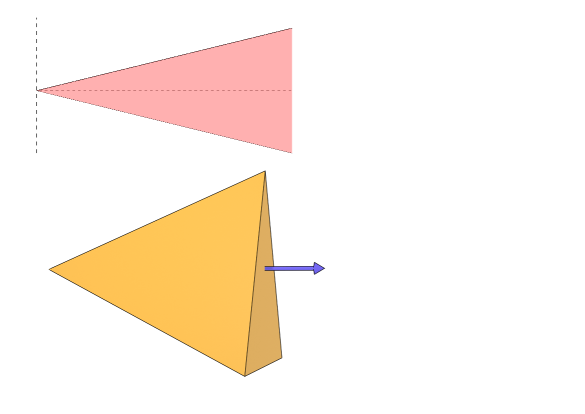
which is a half-space in . The dead set of a layer is just the intersection of the half-space of each neuron, a convex polytope, which is possibly empty or even unbounded. For the sake of simplicity, this paper follows the convention that the number of features is identical in each layer. In this case, the dead set is actually an affine cone, as there is exactly one vertex which is the intersection of linear equations in , except for degenerate cases with probability zero. Furthermore, if we follow the usual practice that at initialization, then the dead set is a convex cone with vertex at the origin, as seen in figure 1.
For convenience, we denote the dead set of the neuron in the layer as , while the dead set of the whole layer is . If , and is the least layer in which this occurs, we say that is killed by that layer. A dead neuron is one for which all of is dead. In turn, a dead layer is one in which all neurons are dead. Finally, a dead network is one for which the final layer is dead, which is guaranteed if any intermediate layer dies.
We use to denote the probability that a network of width features and depth layers is alive, i.e. not dead, the estimation of which is the central study of this work. For convenience in some proofs, we use denote the event that the layer of the network is alive, a function of the parameters . Under this definition, .
3 Upper bound
First, we derive a conservative upper bound on . We know that for all , due to the ReLU nonlinearity. Thus, if layer kills , then it also kills . Now, if and only if none of the parameters are positive. Since the parameters follow symmetric independent distributions, we have .
Next, note that layer is alive only if is, or more formally, . The law of total probability yields the recursive relationship
| (3) |
Then, since is independent of , we have the upper bound
| (4) |
Note that the bound can be sharpened to an exponent of if the bias terms are initialized to zero. For fixed , this is a geometric sequence in . Note the limit is zero, verifying the claim of Lu et al [17].
4 Lower bound
The previous section showed that deep networks die in probability. Luckily, we can bring our networks back to life again if they grow deeper and wider simultaneously. Our insight is to show that, while a deeper network has a higher chance of dead initialization, a wider network has a lower chance. In what follows, we derive a lower bound for from which we compute the minimal width for a given network depth. The basic idea is this: in a living network, for all . Recall from equation 2 that the dead set of a neuron is a sub-level set of a continuous function, thus it is a closed set [14]. Given any point , implies that there exists some neighborhood around which is also not in . This means that a layer is alive so long as it contains a single living point, so a lower bound for the probability of a living layer is the probability of a single point being alive.
It remains to compute the probability of a single point being alive, the compliment of which we denote by , where is the dead set of some neuron. Surprisingly, does not depend on the value of . Given some symmetric distribution of the parameters, we have
| (5) |
Now, the surface can be rewritten as , a hyperplane in . Since this surface has Lebesgue measure zero, its contribution to the integral is negligible. Combining this with the definition of a PDF, we have
| (6) |
Then, change variables to , with Jacobian determinant , and apply the symmetry of to yield
| (7) |
Thus , so . The previous calculation can be understood in a simple way devoid of any formulas: for any half-space containing , the closure of its compliment is equally likely and with probability one, exactly one of these sets contains . Thus, the probability of drawing a half-space containing is the same as the probability of drawing one that does not, so each must have probability .
Finally, if any of the neurons in layer is alive at , then the whole layer is alive. Since these are independent events with probability , . It follows from equation 3 that
| (8) |
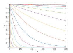
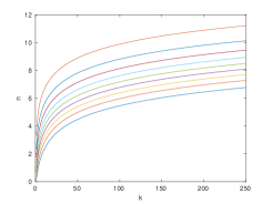
From this inequality, we can compute the width required to achieve as
| (9) |
See figure 2 for plots of these curves for various values of .
5 Tightness of the bounds
Combining the results of the previous sections, we have the bounds
| (10) |
Let denote the lower bound, and the upper. We now show that these bounds are asymptotically tight, as is later verified by our experiments. More precisely, for any , with . Furthermore, along any path such that . This means that these bounds are optimal for the extreme cases of a single-layer network, or a very deep network.
5.1 Tightness of the upper bound for
First we show tightness of the upper bound, for a single-layer network. Note that , so this is equivalent to showing that . This is the case when the input set , and the probability increases to this as the input set grows to fill . This is formalized in the following theorem.
Theorem 5.1.
Let be a sequence of nested sets having as their limit. Let the input set be , the set from this sequence. Then monotonically as .
Proof.
First note that . Next, let with input set . It is easy to verify that this satisfies the axioms of a probability measure. Then we have
whence converge and monotonicity follow from the axioms of measure theory.
∎
5.2 Tightness of the lower bound with contracting input set
Next we show tightness of the lower bound. Recalling that our upper bound is tight for a single-layer network with all of as its input, it stands to reason that the lower bound will be tight for either smaller input sets or more complex models. This intuition is correct, as we will show rigorously in lemma 5.2. In preparation, notice from the derivation of in section 4 that it equals the probability that some data point will be alive in a random network. Owing to the symmetry of the parameter distribution, this does not even depend on the value of , except in the technical case that and the biases are all zero. This furnishes the following theorem, which is verified experimentally by figure 4 in section 6.
Lemma 5.2.
Let . Then the probability that is alive in a -layer network is .
Proof.
The argument is essentially the same as that of section 4. By symmetry, the probability that a is dies in a single neuron is . By independence, the probability that dies in a single layer is . Again by conditional independence, this extends to layers as .
∎
Equipped with this result, it is easy to see that as the input set shrinks in size to a single point. This is made rigorous in the following theorem.
Theorem 5.3.
Let be a sequence of nested sets with limit . Let the input set be , the set from this sequence. Then monotonically as .
Proof.
The proof is the same as that of theorem 5.1, except we take a decreasing sequence. Then, using the same notation as in that proof, . Finally, lemma 5.2 tells us that .
∎
We have shown that when the input set is a single point. Informally, it is easy to believe that as the network grows deeper, for any input set. The previous theorem handles the case that the input set shrinks, and we can often view a deeper layer as one with a shrunken input set, as the network tends to constrict the inputs to a smaller range of values. To formalize this notion, define the living set for parameters as . Then we can state the following lemma and theorem.
Lemma 5.4.
The expected measure of the living set over all possible network parameters is equal to
Theorem 5.5.
Let be a path through hyperparameter space such that is a non-decreasing function of , and . Then as well.
Proof.
For increasing with fixed , note that is a decreasing nested sequence of sets. To move beyond fixed , consider the infinite product space generated by all possible values of , and . In this space, is also a nested decreasing sequence, as is non-decreasing with . By the lemma, implies the limiting set has measure zero. Then, we know that monotonically as well.
Next, recall from section 4 that dead sets are closed, and since the network is continuous we know that is either empty or open, as it is a finite intersection of such sets. Since the input data are drawn from a continuous distribution, it follows that if and only if . Then, we can write
| (11) |
From this formulation, the integrand is monotone in , so by the monotone convergence theorem.
∎
See figure 2 for example paths satisfying the conditions of this theorem. In general, our bounds imply that deeper networks must be wider, so all of practical interest ought to be non-decreasing. This concludes our results from measure theory. In the next section, we adopt a statistical approach to remove the requirement that .
5.3 Tightness of the lower bound as
We have previously shown that converges to the upper bound as the input set grows to with , and that it converges to the lower bound as the input set shrinks to a single point, for any . Finally, we argue that as and increase without limit, without reference to the input set. We have already shown that this holds by an expedient argument in the special case that . In what follows, we drop this assumption and try to establish the result for the general case, substituting an assumption on for one on the statistics of the network outputs.
Assumption 5.6.
Let denote the vector of standard deviations of each element of , which varies with respect to the input data , conditioned on parameters . Let . Assume the sum of normalized conditional variances, taken over all living layers as
| (12) |
has .
This basically states that the normalized variance decays rapidly with the number of layers , and it does not grow too quickly with the number of features . The assumption holds in the numerical simulations of section 6. In what follows, we argue that this is a reasonable assumption, based on some facts about the output variance of a ReLU network.
First we compute the output variance of the affine portion of a ReLU neuron. Assume the input features have zero mean and identity covariance matrix, i.e. the data have undergone a whitening transformation. Let denote the variance of each network parameter, and let denote the output of the neuron in the first layer, with , and parameters defined accordingly. Then
| (13) | ||||
This shows that the pre-ReLU variance does not increase with each layer so long as , the variance used in the Xavier initialization scheme [5]. A similar computation can be applied to later layers, canceling terms involving uncorrelated features.
To show that the variance actually decreases rapidly with , we must factor in the ReLU nonlinearity. The basic intuition is that, as data progresses through a network, information is lost when neurons die. For a deep enough network, the response of each data point is essentially just , which we call the eigenvalue of the network. The following result makes precise this notion of information loss.
Lemma 5.7.
Given a rectifier neuron with input data and parameters , the expected output variance is related to the pre-ReLU variance by
Proof.
From the definition of variance,
| (14) |
Taking the expected value over , we have that , both being equal to . For a symmetric zero-mean parameter distribution we have
| (15) |
As in section 4, symmetry tells us that the integral over is equal to that over , thus Similarly, odd symmetry of yields , so the pre-ReLU variance is just . Combining these results with equation 14 yields the desired result.
∎
This shows that the average variance decays in each layer by a factor of at least , explaining the factor of applied to parameter variances in the He initialization scheme [9]. However, the remaining term shows that a factor of 2 is insufficient, and variance decay will still occur, as seen in the experiments of section 6. This serves both as a principled derivation of He initialization, as well as an elucidation of its weaknesses. While this is not a complete proof of assumption 5.6, it offers strong evidence for geometric variance decay.
After these preliminaries, we can now show the tightness of the lower bound based on assumption 5.6. To simplify the proof, we switch to the perspective of a discrete IID dataset . Let denote the number of living data points at layer , and let . It is a vacuous to study with fixed , as in this case. Similarly, as for fixed . Instead, we consider any path through hyperparameter space, which essentially states that both and grow without limit. For example, consider equation 9 for any , which gives the curve such that . Then, we show that as .
Proof.
Partition the parameter space into the following events, conditioned on :
-
1.
: All remaining data lives at layer :
-
2.
: Only some of the remaining data lives at layer :
-
3.
: All the remaining data is killed: .
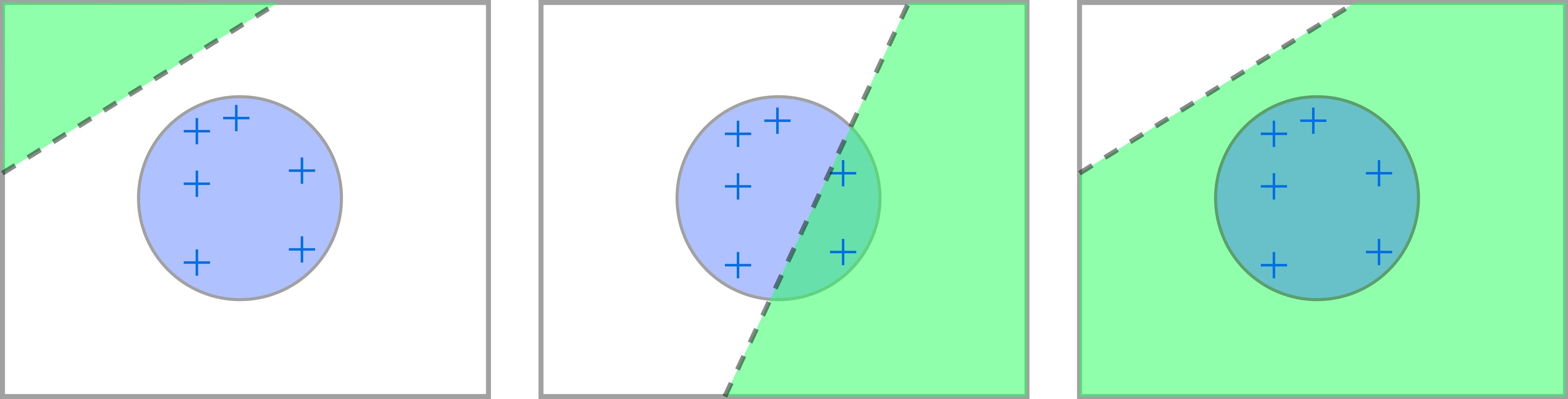
These events are visualized in figure 3. Now, as the events are disjoint, we can write
| (16) |
Now, conditioning on the compliment of means that either all the remaining data is alive or none of it. If none of it, then flipping the sign of any neuron brings all the remaining data to life with probability one. As in section 4, symmetry of the parameter distribution ensures all sign flips are equally likely. Thus . Since and partition , we have
| (17) | ||||
Recall the lower bound Expanding terms in the recursion, and letting be the analogous event for layer , we have that
| (18) |
Now, implies that for some while . But, if and only if . Applying the union bound across data points followed by Chebyshev’s inequality, we have that
| (19) |
Therefore , the sum from assumption 5.6. Now, since all terms in equation 18 are non-negative, we can collect them in the bound
| (20) |
This is a geometric series in , and by assumption 5.6, with .
∎
This concludes our argument for the optimality of our lower bound. Unlike in the previous section, here we required a strong statistical assumption to yield a compact, tidy proof. The truth of assumption 5.6 depends on the distribution of both the input data and the parameters. Note that this is a sufficient rather than necessary condition, i.e. the lower bound might be optimal regardless of the assumption. Note also that assumption 5.6 is a proxy for the more technical condition that the sum is . This means that the probability of the dataset partially dying decreases rapidly with network depth. In other words, for deeper layers, either all the data lives or none of it. There may be other justifications for this result which dispense with the variance, such as the contracting radius of the output set, or the increasing dimensionality of the feature space . We chose to work with the variance because it roughly captures the size of the output set, and is much easier to compute than the geometric radius or spectral norm.
6 Numerical simulations of bounds
We now confirm our previously established bounds on neuron death by numerical simulation. We followed the straightforward methodology of generating a number of random networks, applying these to random data, and computing various statistics on the output. All experiments were conducted using SciPy and required several hours’ compute time on a standard desktop CPU [26].
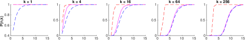
First we generated the random data and networks. Following the typical convention of using white training data, we randomly generated data points from standard normal distributions in , for each feature dimensionality [25]. Then, we randomly initialized fully-connected ReLU networks having layers. Following the popular He initialization scheme, we initialized the multiplicative network parameters with normal distributions having variance , while the additive parameters were initialized to zero [9]. Then, we computed the number of living data points for each network, concluding that a network has died if no living data remain at the output. The results are shown in figure 4 alongside the upper and lower bounds from inequality 10.
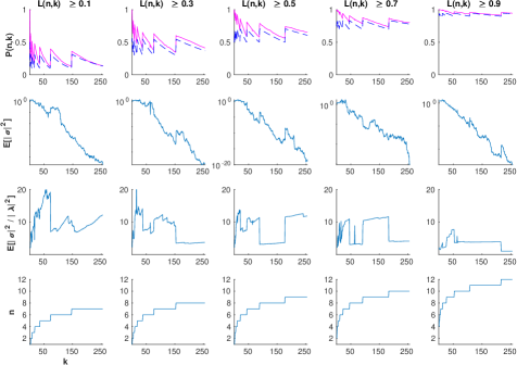
Next, to show asymptotic tightness of the lower bound, we conducted a similar experiment using the hyperparameters defined by equation 9, rounding upwards to the next integer, for various values of . These plots ensure that the lower bound is approximately constant at , while the upper bound is approximately equal to one, that converges to a nontrivial value. The results are shown in figure 5.
We draw two main conclusions from these graphs. First, the simulations agree with our theoretical bounds, as in all cases. Second, the experiments support asymptotic tightness of the lower bound, as with increasing and . Interestingly, the variance decreases exponentially in figure 5, despite the fact that He initialization was designed to stabilize it [9]. This could be explained by the extra term in lemma 5.2. However, we do not notice exponential decay after normalization by the mean , as would be required by assumption 5.6. Recall that assumption 5.6 is a strong claim meant to furnish a sufficient, yet unnecessary condition that . That is, the lower bound might still be optimal even if the assumption is violated, as suggested by the graphs.
7 Sign-flipping and batch normalization
Our previous experiments and theoretical results demonstrated some of the issues with IID ReLU networks. Now, we propose a slight deviation from the usual initialization strategy which partially circumvents the issue of dead neurons. As in the experiments, we switch to a discrete point of view, using a finite dataset . Our key observation is that, with probability one, negating the parameters of a layer revives any data points killed by it. Thus, starting from the first layer, we can count how many data points are killed, and if this exceeds half the number which were previously alive, we negate the parameters of that layer. This alters the joint parameter distribution based on the available data, while preserving the marginal distribution of each parameter. Furthermore, this scheme is practical, costing essentially the same as a forward pass over the dataset.
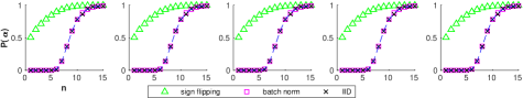
For a -layer network, this scheme guarantees that at least data points live. The caveat is that the pre-ReLU output cannot be all zeros, or else negating the parameters would not change the output. However, this edge case has probability zero since depends on a polynomial in the parameters of layer , the roots of which have measure zero. Batch normalization provides a similar guarantee: if for all , then with probability one there is at least one living data point [12]. Similar to our sign-flipping scheme, this prevents total network death while still permitting individual data points to die.
These two schemes are simulated and compared in figure 6. Note that for IID data , as that bound comes from the probability that any random data point is alive. Sign-flipping significantly increased the proportion of living data, far exceeding the fraction that is theoretically guaranteed. In contrast, batch normalization ensured that the network was alive, but did nothing to increase the proportion of living data over our IID baseline.
8 Implications for network design
Neuron death is not only relevant for understanding how to initialize a very deep neural network, but also helps to explain various aspects of the model architecture itself. Equation 9 in section 4 tells us how wide a -layer network needs to be; if a network is deep and skinny, most of the data will die. We have also seen in section 7 that batch normalization prevents neuron death, supplementing the existing explanations of its efficacy [22]. Surprisingly, many other innovations in network design can also be viewed through the lens of neuron death.
Up to this point we focused on fully-connected ReLU networks. Here we briefly discuss how our results generalize to other network types. Interestingly, many of the existing network architectures bear relevance in preventing neuron death, even if they were not originally designed for this purpose. What follows is meant to highlight the major categories of feed-forward models, but our list is by no means exhaustive.
8.1 Convolutional networks
Convolutional neural networks (CNNs) are perhaps the most popular type of artificial neural network. Specialized for image and signal processing, these networks have most of their neurons constrained to perform convolutions. Keeping with our previous conventions, we say that a convolutional neuron takes in feature maps and computes
| (21) |
where the maximum is again taken element-wise. In the two-dimensional case, and . By the Riesz Representation Theorem, discrete convolution can be represented by multiplication with some matrix . Since is a function of the much smaller matrix , we need to rework our previous bounds in terms of the dimensions and . It can be shown by similar arguments that
| (22) |
Compare this to inequality 10. As with fully-connected networks, the lower bound depends on the number of neurons, while the upper bound depends on the total number of parameters. To our knowledge, the main results of this work apply equally well to convolutional networks; the fully-connected type was used only for convenience.
8.2 Residual networks and skip connections
Residual networks (ResNets) are composed of layers which add their input features to the output [10]. Residual connections do not prevent neuron death, as attested by other recent work [1]. However, they do prevent a dead layer from automatically killing any later ones, by creating a path around it. This could explain how residual connections allow deeper networks to be trained [10]. The residual connection may also affect the output variance and prevent information loss.
A related design feature is the use of skip connections, as in fully-convolutional networks [23]. For these architectures, the probability of network death is a function of the shortest path through the network. In many segmentation models this path is extremely short. For example, in the popular U-Net architecture, with chunk length , the shortest path has a depth of only [21]. This means that the network can continue to function even if the innermost layers are disabled.
8.3 Other nonlinearities
This work focuses on the properties of the ReLU nonlinearity, but others are sometimes used including the leaky ReLU, “swish” and hyperbolic tangent [4, 19]. With the exception of the sigmoid type, all these alternatives retain the basic shape of the ReLU, with only slight modifications to increase smoothness or prevent neuron death. For all of these functions, part of the input domain is much less sensitive than the rest. In the sigmoid type it is the extremes of the input space, while in the ReLU variants it the negatives. Our theory easily extends to all the ReLU variants by replacing dead data points with weak ones, i.e. those with small gradients. Given that gradients are averaged over a mini-batch, weak data points are likely equivalent to dead ones in practice [7]. We suspect this practical equivalence is what allows the ReLU variants to maintain similar performance levels to the original [19].
9 Conclusions
We have established several theoretical results concerning ReLU neuron death, confirmed these results experimentally, and discussed their implications for network design. The main results were an upper and lower bound for the probability of network death , in terms of the network width and depth . We provided several arguments for the asymptotic tightness of these bounds. From the lower bound, we also derived a formula relating network width to depth in order to guarantee a desired probability of living initialization. Finally, we showed that our lower bound coincides with the probability of data death, and developed a sign-flipping initialization scheme to reduce this probability.
We have seen that neuron death is a deep topic covering many aspects of neural network design. This article only discusses what happens at random initialization, and much more could be said about the complex dynamics of training a neural network [1, 27]. We do not claim that neuron death offers a complete explanation of any of these topics. On the contrary, it adds to the list of possible explanations, one of which may someday rise to preeminence. Even if neuron death proves unimportant, it may still correlate to some other quantity with a more direct relationship to model efficacy. In this way, studying neuron death could lead to the discovery of other important factors, such as information loss through a deep network. At any rate, the theory of deep learning undoubtedly lags behind the recent advances in practice, and until this trend reverses, every avenue is deserving of exploration.
References
- [1] Isac Arnekvist, J. Frederico Carvalho, Danica Kragic, and Johannes A. Stork. The effect of target normalization and momentum on dying relu. cs.LG, arXiv:2005.06195, 2020.
- [2] Randall Balestriero, Romain Cosentino, Behnaam Aazhang, and Richard Baraniuk. The geometry of deep networks: Power diagram subdivision. In NeurIPS, 2019.
- [3] Qishang Cheng, HongLiang Li, Qingbo Wu, Lei Ma, and King Ngi Ngan. Parametric deformable exponential linear units for deep neural networks. Neural Networks, 125:281 – 289, 2020.
- [4] Djork-Arné Clevert, Thomas Unterthiner, and Sepp Hochreiter. Fast and accurate deep network learning by exponential linear units (elus). In Yoshua Bengio and Yann LeCun, editors, ICLR, 2016.
- [5] Xavier Glorot and Y. Bengio. Understanding the difficulty of training deep feedforward neural networks. Journal of Machine Learning Research - Proceedings Track, 9:249–256, 01 2010.
- [6] Xavier Glorot, Antoine Bordes, and Yoshua Bengio. Deep sparse rectifier neural networks. In Geoffrey J. Gordon and David B. Dunson, editors, AISTATS, volume 15, pages 315–323. Journal of Machine Learning Research - Workshop and Conference Proceedings, 2011.
- [7] Ian Goodfellow, Yoshua Bengio, and Aaron Courville. Deep Learning. MIT Press, 2016. http://www.deeplearningbook.org.
- [8] Ian Goodfellow, David Warde-Farley, Mehdi Mirza, Aaron Courville, and Yoshua Bengio. Maxout networks. In PMLR, volume 28, pages 1319–1327, 2013.
- [9] K. He, X. Zhang, S. Ren, and J. Sun. Delving deep into rectifiers: Surpassing human-level performance on imagenet classification. In IEEE International Conference on Computer Vision (ICCV), pages 1026–1034, 2015.
- [10] K. He, X. Zhang, S. Ren, and J. Sun. Deep residual learning for image recognition. In 2016 IEEE Conference on Computer Vision and Pattern Recognition (CVPR), pages 770–778, 2016.
- [11] Frank Hutter, Lars Kotthoff, and Joaquin Vanschoren, editors. Automated Machine Learning: Methods, Systems, Challenges. Springer, 2018. In press, available at http://automl.org/book.
- [12] Sergey Ioffe and Christian Szegedy. Batch normalization: Accelerating deep network training by reducing internal covariate shift. In ICML, volume 37, pages 448 – 456. JMLR.org, 2015.
- [13] Fabian Isensee, Paul F. Jaeger, Simon A. A. Kohl, Jens Petersen, and Klaus H. Maier-Hein. nnU-Net: a self-configuring method for deep learning-based biomedical image segmentation. Nature Methods, 18(2):203–211, 2021.
- [14] Richard Johnsonbaugh and W. E. Pfaffenberger. Foundations of Mathematical Analysis. Marcel Dekker, New York, New York, USA, Dover 2002 edition, 1981.
- [15] Alex Krizhevsky, Ilya Sutskever, and Geoffrey E. Hinton. ImageNet classification with deep convolutional neural networks. In NIPS, 2012.
- [16] Yann A. LeCun, Léon Bottou, Genevieve B. Orr, and Klaus-Robert Müller. Efficient backprop. In Neural Networks: Tricks of the Trade: Second Edition, pages 9–48. Springer Berlin Heidelberg, 2012.
- [17] Lu Lu, Yeonjong Shin, Yanhui Su, and George Em Karniadakis. Dying relu and initialization: Theory and numerical examples. stat.ML, arXiv:1903.06733, 2019.
- [18] Guido Montufar, Razvan Pascanu, Kyunghyun Cho, and Y. Bengio. On the number of linear regions of deep neural networks. 2014.
- [19] Prajit Ramachandran, Barret Zoph, and Quoc V. Le. Searching for activation functions. In ICLR, 2018.
- [20] Blaine Rister and Daniel L. Rubin. Piecewise convexity of artificial neural networks. Neural Networks, 94:34 – 45, 2017.
- [21] Olaf Ronneberger, Philipp Fischer, and Thomas Brox. U-net: Convolutional networks for biomedical image segmentation. In Medical Image Computing and Computer-Assisted Intervention – MICCAI, pages 234–241, Cham, 2015.
- [22] Shibani Santurkar, Dimitris Tsipras, Andrew Ilyas, and Aleksander Madry. How does batch normalization help optimization? In S. Bengio, H. Wallach, H. Larochelle, K. Grauman, N. Cesa-Bianchi, and R. Garnett, editors, Advances in Neural Information Processing Systems, volume 31. Curran Associates, Inc., 2018.
- [23] E. Shelhamer, J. Long, and T. Darrell. Fully convolutional networks for semantic segmentation. IEEE Transactions on Pattern Analysis and Machine Intelligence, 39(4):640–651, April 2017.
- [24] Yeonjong Shin and George E. Karniadakis. Trainability and data-dependent initialization of over-parameterized relu neural networks. CoRR, arXiv:1907.09696, 2019.
- [25] J. Sola and J. Sevilla. Importance of input data normalization for the application of neural networks to complex industrial problems. IEEE Transactions on Nuclear Science, 44(3):1464–1468, 1997.
- [26] Pauli Virtanen, Ralf Gommers, Travis E. Oliphant, Matt Haberland, Tyler Reddy, David Cournapeau, Evgeni Burovski, Pearu Peterson, Warren Weckesser, Jonathan Bright, Stéfan J. van der Walt, Matthew Brett, Joshua Wilson, K. Jarrod Millman, Nikolay Mayorov, Andrew R. J. Nelson, Eric Jones, Robert Kern, Eric Larson, C J Carey, İlhan Polat, Yu Feng, Eric W. Moore, Jake VanderPlas, Denis Laxalde, Josef Perktold, Robert Cimrman, Ian Henriksen, E. A. Quintero, Charles R. Harris, Anne M. Archibald, Antônio H. Ribeiro, Fabian Pedregosa, Paul van Mulbregt, and SciPy 1.0 Contributors. SciPy 1.0: Fundamental Algorithms for Scientific Computing in Python. Nature Methods, 17:261–272, 2020.
- [27] Yueh-Hua Wu, Fan-Yun Sun, Yen-Yu Chang, and Shou-De Lin. ANS: Adaptive network scaling for deep rectifier reinforcement learning models. cs.LG, arxiv:1809.02112, 2018.