This paper was converted on www.awesomepapers.org from LaTeX by an anonymous user.
Want to know more? Visit the Converter page.

Probabilistic Reduced-Dimensional Vector Autoregressive Modeling with Oblique Projections

Yanfang Mo yanfang.mo@cityu.edu.hk    S. Joe Qin joeqin@LN.edu.hk Hong Kong Institute for Data Science, City University of Hong Kong, Hong Kong The Institute of Data Science, Lingnan University, Hong Kong
?abstractname?

In this paper, we propose a probabilistic reduced-dimensional vector autoregressive (PredVAR) model to extract low-dimensional dynamics from high-dimensional noisy data. The model utilizes an oblique projection to partition the measurement space into a subspace that accommodates the reduced-dimensional dynamics and a complementary static subspace. An optimal oblique decomposition is derived for the best predictability regarding prediction error covariance. Building on this, we develop an iterative PredVAR algorithm using maximum likelihood and the expectation-maximization (EM) framework. This algorithm alternately updates the estimates of the latent dynamics and optimal oblique projection, yielding dynamic latent variables with rank-ordered predictability and an explicit latent VAR model that is consistent with the outer projection model. The superior performance and efficiency of the proposed approach are demonstrated using data sets from a synthesized Lorenz system and an industrial process from Eastman Chemical.

keywords:
Identification and model reduction; process control; estimation; statistical learning
thanks: The work described in this paper was partially supported by a grant from a General Research Fund by the Research Grants Council (RGC) of Hong Kong SAR, China (Project No. 11303421), a Collaborative Research Fund by RGC of Hong Kong (Project No. C1143-20G), a grant from the Natural Science Foundation of China (U20A20189), a grant from ITF - Guangdong-Hong Kong Technology Cooperation Funding Scheme (Project Ref. No. GHP/145/20), a Math and Application Project (2021YFA1003504) under the National Key R&D Program, a Shenzhen-Hong Kong-Macau Science and Technology Project Category C (9240086), and an InnoHK initiative of The Government of the HKSAR for the Laboratory for AI-Powered Financial Technologies. Part of the material in this paper was presented at the 62nd IEEE Conference on Decision and Control, December 13–15, 2023, Singapore [22]. (Corresponding author: S. J. Qin)

, and

1 Introduction

With the popular deployment of the industrial internet of things, high-dimensional data with low-dimensional dynamics [35] pose new challenges to traditional time series analysis methods that assume fully excited full-dimensional dynamics. In many real industrial operations, high dimensional time series often do not exhibit full-dimensional dynamics [25]. In addition, autonomous systems deploy redundant sensors for safety and fault tolerance, resulting in high collinearity in the collected time-series data. Moreover, computationally intensive applications like digital twins produce high dimensional data to capture important dynamics for effective decision-making [13]. These popular application scenarios call for parsimonious modeling to extract reduced-dimensional dynamics in high dimensional data [30, 32].

Classic reduced-dimensional analytic tools, such as principal component analysis (PCA), partial least squares (PLS) [15, 31], and canonical correlation analysis (CCA), have been successful in many applications. While they perform dimension reduction, their statistical inference requires serial independence in the data [30].

Many efforts in the statistical field have raised the issue of reduced dimensional dynamics in multivariate time series data. An early account of this problem is given in [3], which does the dynamics modeling and dimensional reduction in two steps and thus is not optimal. Subsequently, dynamic factor models (DFMs) are developed, which rely on time-related statistics to estimate parsimonious model parameters, including [25, 18, 26, 14]. However, these DFMs do not enforce a parsimonious latent dynamic model. The linear Gaussian state-space model in [37] and the autoregressive DLV model in [41] extract the dynamic and static characteristics simultaneously. Nevertheless, they ignore the structured signal-noise relationship and are not concerned with the dimension reduction in noise.

In process data analytics, a dynamic latent variable (DLV) model was developed in [19] to extract DLVs first and characterize the dynamic relations in the DLVs and the static cross-correlations in residuals afterward. Assuming the latent dynamics is integrating or being ‘slow’, slow feature analysis has been developed [40, 33, 11] to induce dimension reduction focusing on slow dynamics only. To develop full latent dynamic features, dynamic-inner PCA (DiPCA) [10] and dynamic-inner CCA (DiCCA) [9, 8] are proposed to produce rank-ordered DLVs to maximize the prediction power in terms of covariance and canonical correlation, respectively. Furthermore, Qin developed a latent vector autoregressive modeling algorithm with a CCA objective (LaVAR-CCA) [28, 29], whose state-space generalization is developed in [38]. Casting the LaVAR model in a probabilistic setting, [12] uses the Kalman filter formulation to solve for the dynamic and static models via maximum likelihood, but fails short of solving the dynamic model parameters explicitly and resorts to genetic algorithms for the solution. A key to signal reconstruction and prediction lies in separating the serially dependent signals from serially independent noise that may have energy or variance comparable to that of the signals [30].

The prevalence of low-dimensional dynamics in high-dimensional uncertainties requires a statistical framework for simultaneous dimension reduction and latent dynamics extraction. In this paper, we propose a probabilistic reduced-dimensional vector autoregressive (PredVAR) model to extract low-dimensional dynamics from high-dimensional noisy data. Our probabilistic model partitions the measurement space into a low-dimensional DLV subspace and a static noise subspace, which are generally oblique. An oblique projection is adopted to delineate the structural signal-noise relationship, extending the widely used orthogonal projection [21]. The oblique projection for the dynamic-static decomposition in our model is found simultaneously with an explicit low-dimensional latent dynamic model. Accordingly, our model consists of two interrelated components, namely, the optimal oblique projection and the latent dynamics. An expectation-maximization (EM) procedure is used to estimate model parameters [7, 39] that satisfy the maximum likelihood optimal conditions.

The main contributions of this work are as follows.

1)1) A probabilistic reduced-dimensional vector regressive (PredVAR) model is proposed with general oblique projections. Our study of using VAR to capture latent dynamics should initiate exploring more dynamic models.

2)2) A particular oblique projection is derived for the optimal dynamic-static decomposition, which achieves the best predictability regarding prediction error covariance and has an intriguing geometric interpretation. Also, ordered DLVs are obtained based on predictability.

3)3) A PredVAR model identification algorithm is developed based on the optimal dynamic-static decomposition, the interplay between latent dynamics and projection identifications, and the EM method. The noise covariance matrices are estimated as a byproduct of the EM method and the analytical comparison with LaVAR-CCA and DiCCA naturally follows.

4)4) Extensive simulations are presented to illustrate our approach compared to conceivable benchmarks over the synthesized Lorenz data and real Eastman process data.

The rest of the paper is organized as follows. The PredVAR model is formulated in Section 2. An efficient PredVAR model identification algorithm is developed in Section 3, based on the optimal dynamic-static decomposition introduced in Section 4. Additional analysis is presented in Section 5, including the distributions of parameter estimates and the selection of model sizes. Section 6 presents simulation comparison and studies. Finally, this paper is concluded in Section 7. Table 1 summarizes the major notation.

?tablename? 1: Notation.
n{\llbracket n\rrbracket} {1,2,,n}\{1,2,\ldots,n\} for a natural number nn
ss order of the vector autoregressive (VAR) dynamics
pp dimension of the measurement space
\ell dynamic latent dimension (DLD)
𝒚k\bm{y}_{k} measurement vector in p\Re^{p}
𝒗k\bm{v}_{k} Dynamic latent variables (DLVs) in \Re^{\ell}
𝒗^k\bm{\hat{v}}_{k} one-step ahead DLVs prediction in \Re^{\ell}
𝜺k\bm{\varepsilon}_{k} DLV innovations vector in \Re^{\ell}, 𝜺k𝒩(𝟎,𝚺𝜺)\bm{\varepsilon}_{k}\sim\mathcal{N}(\bm{0},\mathbf{\Sigma}_{\bm{\varepsilon}})
𝜺¯k\bm{\bar{\varepsilon}}_{k} outer model noise in p\Re^{p-\ell}, 𝜺¯k𝒩(𝟎,𝚺𝜺¯)\bm{\bar{\varepsilon}}_{k}\sim\mathcal{N}(\bm{0},\mathbf{\Sigma}_{\bm{\bar{\varepsilon}}})
𝒆k\bm{e}_{k} innovations vector in p\Re^{p}𝒆k=𝐏𝜺k+𝐏¯𝜺¯k\bm{e}_{k}=\mathbf{P}\bm{\varepsilon}_{k}+\mathbf{\bar{P}}\bm{\bar{\varepsilon}}_{k}
𝐈/𝟎\mathbf{I}/\bm{0} identity/zero matrix of a compatible dimension
𝐁j\mathbf{B}_{j} VAR coefficient matrix in ×\Re^{\ell\times\ell}, jsj\in{\llbracket s\rrbracket}
𝐏\mathbf{P} DLV loadings matrix in p×\Re^{p\times\ell}
𝐏¯\mathbf{\bar{P}} static loadings matrix in p×(p)\Re^{p\times{(p-\ell)}}
𝐑\mathbf{R} DLV weight matrix in p×\Re^{p\times\ell}
𝐑¯\mathbf{\bar{R}} static weight matrix in p×(p)\Re^{p\times{(p-\ell)}}
𝚺\mathbf{\Sigma}_{\bm{*}} covariance matrix of a random vector \bm{*}

2 Model Formulation

2.1 The PredVAR Model

Consider a time series {𝒚kp}k=1N+s\{\bm{y}_{k}\in\Re^{p}\}_{k=1}^{N+s} with E(𝒚k)=𝟎E(\bm{y}_{k})=\bm{0} for all kN+sk\in{\llbracket N+s\rrbracket}. Qin [29] defines that the time series is serially correlated or dynamic if, for at least one j>0j>0,

E{𝒚k𝒚kj}𝟎.{E}\left\{\bm{y}_{k}\bm{y}_{k-j}^{\intercal}\right\}\neq\mathbf{0}.

Otherwise, it is serially uncorrelated. Further, as per Qin [29], {𝒚k}\{\bm{y}_{k}\} is a reduced-dimensional dynamic (RDD) series if it is serially correlated but {𝐚𝒚k}\{\mathbf{a}^{\intercal}\boldsymbol{y}_{k}\} is serially uncorrelated for some 𝐚𝟎p\mathbf{a\neq 0}\in\Re^{p}. If no 𝐚𝟎\mathbf{a\neq 0} exists to render {𝐚𝒚k}\{\mathbf{a}^{\intercal}\bm{y}_{k}\} serially uncorrelated, {𝒚k}\{\bm{y}_{k}\} is full-dimensional dynamic (FDD). Qin [29] develops a latent VAR model to estimate the RDD dynamics of the data series. However, no statistical analysis is given since the latent VAR model does not give the distributions of noise terms.

Refer to caption
?figurename? 1: A block diagram of a PredVAR model.

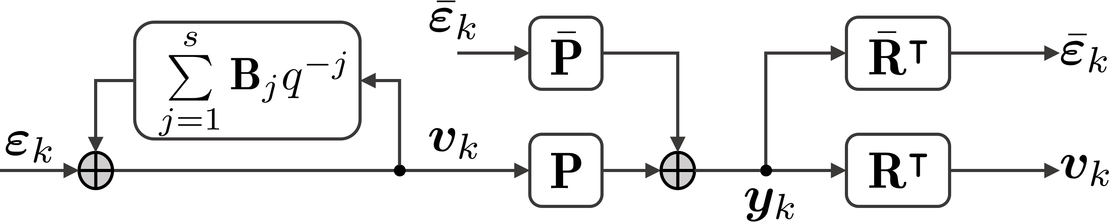
In this paper, we define a probabilistic reduced-dimensional vector autoregressive series as

𝒚k=𝐏𝒗k+𝐏¯𝜺¯k,\displaystyle\bm{y}_{k}=\mathbf{P}\bm{v}_{k}+\mathbf{\bar{P}}\bm{\bar{\varepsilon}}_{k}, 𝜺¯k𝒩(𝟎,𝚺𝜺¯),\displaystyle\bm{\bar{\varepsilon}}_{k}\sim\mathcal{N}(\bm{0},\mathbf{\Sigma}_{\bm{\bar{\varepsilon}}}), (1)
𝒗k=j=1s𝐁j𝒗kj+𝜺k,\displaystyle\bm{v}_{k}=\sum_{j=1}^{s}\mathbf{B}_{j}\bm{v}_{k-j}+\bm{\varepsilon}_{k},\leavevmode\nobreak\ \leavevmode\nobreak\ 𝜺k𝒩(𝟎,𝚺𝜺),\displaystyle\bm{\varepsilon}_{k}\sim\mathcal{N}(\bm{0},\mathbf{\Sigma}_{\bm{\varepsilon}}), (2)

where {𝜺k}\{\bm{\varepsilon}_{k}\} and {𝜺¯k}\{\bm{\bar{\varepsilon}}_{k}\} are i.i.d. Gaussian noise terms and 𝒗k\bm{v}_{k}\in\Re^{\ell} denotes the vector of \ell DLVs. Both 𝜺j\bm{\varepsilon}_{j} and 𝜺¯j\bm{\bar{\varepsilon}}_{j} form the innovations and therefore are uncorrelated with the past 𝒗i\bm{v}_{i} for all i<ji<j. With <p\ell<p, the loadings matrices 𝐏p×\mathbf{P}\in\Re^{p\times\ell}, 𝐏¯p×(p)\mathbf{\bar{P}}\in\Re^{p\times(p-\ell)}, and [𝐏𝐏¯]p×p\left[\mathbf{P}\leavevmode\nobreak\ \leavevmode\nobreak\ \mathbf{\bar{P}}\right]\in\Re^{p\times p} have full rank. Using the backward-shift operator q1q^{-1}, the latent dynamic system (2) can be converted to

𝒗k=(𝐈j=1s𝐁jqj)1𝜺k=𝐆v(q1)𝜺k.\bm{v}_{k}=\left(\mathbf{I}-\sum_{j=1}^{s}\mathbf{B}_{j}q^{-j}\right)^{-1}\bm{\varepsilon}_{k}=\mathbf{G}_{v}(q^{-1})\bm{\varepsilon}_{k}.

Then, the transfer matrix form of (1)–(2) is given by

𝒚k=[𝐏𝐏¯][𝐆v(q1)𝟎𝟎𝐈][𝜺k𝜺¯k]\displaystyle\bm{y}_{k}=\left[\mathbf{P}\leavevmode\nobreak\ \leavevmode\nobreak\ \mathbf{\bar{P}}\right]\begin{bmatrix}\mathbf{G}_{v}(q^{-1})&\mathbf{0}\\ \mathbf{0}&\mathbf{I}\end{bmatrix}\begin{bmatrix}\bm{\varepsilon}_{k}\\ \bm{\bar{\varepsilon}}_{k}\end{bmatrix}

which clearly shows the reduced-dimensional dynamics that are commonly observed in routine operational data [29] and economics [34, 14]. Further, for weakly FDD time series, an RDD approximation is often useful to enable rapid downstream decision-making [13]. It should be noted that the latent VAR model (2) can be replaced by a state-space, an ARIMA, or a kernel-based model [8, 38, 27, 17].

2.2 Explicit Expression of DLVs

The PredVAR model (1)–(2) is uniquely characterized by the tuple {𝐏,{𝐁j},𝐏¯}\{\mathbf{P},\{\mathbf{B}_{j}\},\mathbf{\bar{P}}\}, but it is implicit in the DLVs 𝒗k\bm{v}_{k}. To yield an explicit expression of 𝒗k\bm{v}_{k}, define 𝐑p×\mathbf{R}\in\Re^{p\times\ell} and 𝐑¯p×(p)\mathbf{\bar{R}}\in\Re^{p\times(p-\ell)} such that

[𝐑𝐑¯][𝐏𝐏¯]=𝐈,\left[\mathbf{R}\leavevmode\nobreak\ \leavevmode\nobreak\ \mathbf{\bar{R}}\right]^{\intercal}\left[\mathbf{P}\leavevmode\nobreak\ \leavevmode\nobreak\ \mathbf{\bar{P}}\right]=\mathbf{I}, (3)

which makes [𝐑𝐑¯]\left[\mathbf{R}\leavevmode\nobreak\ \leavevmode\nobreak\ \mathbf{\bar{R}}\right] unique given 𝐏\mathbf{P} and 𝐏¯\mathbf{\bar{P}}. The relation (3) also implies

𝐑𝐏=𝐈,𝐑𝐏¯=𝟎,𝐏𝐑+𝐏¯𝐑¯=𝐈,\mathbf{R}^{\intercal}\mathbf{P}=\mathbf{I},\quad\mathbf{R}^{\intercal}\mathbf{\bar{P}}=\mathbf{0},\quad\mathbf{P}\mathbf{R}^{\intercal}+\mathbf{\bar{P}}\mathbf{\bar{R}}^{\intercal}=\mathbf{I},

where 𝐏𝐑\mathbf{P}\mathbf{R}^{\intercal} and 𝐏¯𝐑¯\mathbf{\bar{P}}\mathbf{\bar{R}}^{\intercal} are two oblique projection matrices because (𝐏𝐑)2=𝐏𝐑(\mathbf{P}\mathbf{R}^{\intercal})^{2}=\mathbf{P}\mathbf{R}^{\intercal} and (𝐏¯𝐑¯)2=𝐏¯𝐑¯(\mathbf{\bar{P}}\mathbf{\bar{R}}^{\intercal})^{2}=\mathbf{\bar{P}}\mathbf{\bar{R}}^{\intercal}.

The pair (𝐑,𝐑¯)(\mathbf{R},\mathbf{\bar{R}}) gives explicitly the DLVs 𝒗k\bm{v}_{k} and the static noise 𝜺¯𝒌\bm{\bar{\varepsilon}_{k}} from (1),

𝒗k\displaystyle\bm{v}_{k} =𝐑𝒚k,\displaystyle=\mathbf{R}^{\intercal}\bm{y}_{k}, (4)
𝜺¯k\displaystyle\bm{\bar{\varepsilon}}_{k} =𝐑¯𝒚k.\displaystyle=\mathbf{\bar{R}}^{\intercal}\bm{y}_{k}. (5)

Equations (4) and (5) jointly explain the dynamic-static decomposition of 𝒚k\bm{y}_{k} and reversely (1) gives the composition of 𝒚k\bm{y}_{k}. The reversible relations and the PredVAR model are depicted in Fig. 1 with a block diagram.

2.3 Identifiability of the PredVAR Model

Given any pair of nonsingular matrices 𝐌¯(p)×(p)\mathbf{\bar{M}}\in\Re^{(p-\ell)\times(p-\ell)} and 𝐌×\mathbf{M}\in\Re^{\ell\times\ell}, (1) can be rewritten as

𝒚k\displaystyle\bm{y}_{k} =𝐏𝒗k+𝐏¯𝜺¯k=𝐏𝐌1𝐌𝒗k+𝐏¯𝐌¯1𝐌¯𝜺¯k,\displaystyle=\mathbf{P}\bm{v}_{k}+\mathbf{\bar{P}}\bm{\bar{\varepsilon}}_{k}=\mathbf{P}\mathbf{M}^{-1}\mathbf{M}\bm{v}_{k}+\mathbf{\bar{P}}\mathbf{\bar{M}}^{-1}\mathbf{\bar{M}}\bm{\bar{\varepsilon}}_{k}, (6)

which indicates that the tuple (𝐏,𝒗k,𝐏¯,𝜺¯k)(\mathbf{P},\bm{v}_{k},\mathbf{\bar{P}},\bm{\bar{\varepsilon}}_{k}) cannot be uniquely identified since it can be exactly represented by (𝐏𝐌1,𝐌𝒗k,𝐏¯𝐌¯1,𝐌¯𝜺¯k)(\mathbf{P}\mathbf{M}^{-1},\mathbf{M}\bm{v}_{k},\mathbf{\bar{P}}\mathbf{\bar{M}}^{-1},\mathbf{\bar{M}}\bm{\bar{\varepsilon}}_{k}). However, all equivalent realizations differ by similarity transformation only.

The non-uniqueness of the matrices offers the flexibility to extract desired coordinates or features of the DLVs. For example, we can enforce the following conditions to achieve identifiability.

  1. 1.

    𝐏\mathbf{P} orthogonal or the covariance 𝚺𝒗=𝐈\mathbf{\Sigma}_{\bm{v}}=\mathbf{I} or diagonal, and independently,

  2. 2.

    𝐏¯\mathbf{\bar{P}} orthogonal or the covariance 𝚺𝜺¯=𝐈\mathbf{\Sigma}_{\bm{\bar{\varepsilon}}}=\mathbf{I} or diagonal if 𝚺𝜺¯\mathbf{\Sigma}_{\bm{\bar{\varepsilon}}} is non-singular.

  3. 3.

    If 𝚺𝜺¯\mathbf{\Sigma}_{\bm{\bar{\varepsilon}}} is singular, we can represent 𝜺¯k=𝐐𝜺¯k\bm{\bar{\varepsilon}}_{k}=\mathbf{Q}\bm{\bar{\varepsilon}}_{k}^{*} with 𝐐\mathbf{Q} being full-column rank and 𝚺𝜺¯=𝐈\mathbf{\Sigma}_{\bm{\bar{\varepsilon}}^{*}}=\mathbf{I} having a lower dimension than 𝚺𝜺¯\mathbf{\Sigma}_{\bm{\bar{\varepsilon}}}.

In this paper, however, the DLV and static loadings matrices 𝐏\mathbf{P} and 𝐏¯\mathbf{\bar{P}} need not be mutually orthogonal, requiring an oblique projection for the DLV modeling.

These options have been used in the literature to enforce diagonal 𝚺𝜺¯\mathbf{\Sigma}_{\bm{\bar{\varepsilon}}} and 𝚺𝜺\mathbf{\Sigma}_{\bm{\varepsilon}} as in [2], which does not consider rank-deficient innovations, or enforce 𝚺𝒗=𝐈\mathbf{\Sigma}_{\bm{v}}=\mathbf{I} as in [29] to achieve the CCA objective. Further, the DLVs in [29] are arranged in a non-increasing order of predictability. A rank-deficient 𝚺𝜺¯\mathbf{\Sigma}_{\bm{\bar{\varepsilon}}} corresponds to a rank-deficient 𝚺𝒚\mathbf{\Sigma}_{\bm{y}}, which is studied in this paper. These freedoms allow us to obtain desirable realizations of the PredVAR model.

2.4 Equivalent Reduced-Rank VAR Models

A reduced-rank VAR (RRVAR) model is specified as follows: instead of estimating a full-rank coefficient matrix for each lag in a regular VAR model, we impose a factor structure on the coefficient matrices, such that they can be written as a product of lower-rank matrices, namely,

𝒚k=j=1s𝐏´𝐁´j𝐑´𝒚kj+𝒆k,𝒆k𝒩(𝟎,𝚺𝒆),\bm{y}_{k}=\sum_{j=1}^{s}\mathbf{\acute{P}}\mathbf{\acute{B}}_{j}\mathbf{\acute{R}}^{\intercal}\bm{y}_{k-j}+\bm{e}_{k},\leavevmode\nobreak\ \leavevmode\nobreak\ \bm{e}_{k}\sim\mathcal{N}(\bm{0},\mathbf{\Sigma}_{\bm{e}}), (7)

where 𝐑´𝐏´×\mathbf{\acute{R}}^{\intercal}\mathbf{\acute{P}}\in\Re^{\ell\times\ell} is invertible with <p\ell<p and 𝒆kp\bm{e}_{k}\in\Re^{p} is the full-dimensional innovations vector driving {𝒚k}\{\bm{y}_{k}\}.

The reduced-rank VAR is analogous to the reduced-rank regression (RRR) for linear regression [16, 32]. Just as RRR requires specific solutions that differ from ordinary least squares, RRVAR also requires a specific solution differing from that of regular VAR. Theorem 1 shows that the PredVAR and RRVAR models are equivalent.

Theorem 1.

Equivalent canonical RRVAR of the PredVAR model (1).

  1. 1.

    The PredVAR model (1)–(2) is equivalent to the following canonical RRVAR model

    𝒚k=j=1s𝐏𝐁j𝐑𝒚kj+𝒆k,𝒆k𝒩(𝟎,𝚺𝒆)\bm{y}_{k}=\sum_{j=1}^{s}\mathbf{P}\mathbf{B}_{j}\mathbf{R}^{\intercal}\bm{y}_{k-j}+\bm{e}_{k},\leavevmode\nobreak\ \leavevmode\nobreak\ \bm{e}_{k}\sim\mathcal{N}(\bm{0},\mathbf{\Sigma}_{\bm{e}}) (8)

    with 𝐑𝐏=𝐈\mathbf{R}^{\intercal}\mathbf{P}=\mathbf{I} and the innovation 𝒆j\bm{e}_{j} is uncorrelated with 𝒚i\bm{y}_{i} for all i<ji<j.

  2. 2.

    Each RRVAR model (7) can be converted to the canonical RRVAR model (8) with 𝐑𝐏=𝐈\mathbf{R}^{\intercal}\mathbf{P}=\mathbf{I} by setting 𝐏=𝐏´\mathbf{P}=\mathbf{\acute{P}}, 𝐁j=𝐁´j𝐑´𝐏´\mathbf{B}_{j}=\mathbf{\acute{B}}_{j}\mathbf{\acute{R}}^{\intercal}\mathbf{\acute{P}}, and 𝐑=𝐑´(𝐏´𝐑´)1\mathbf{R}=\mathbf{\acute{R}}(\mathbf{\acute{P}}^{\intercal}\mathbf{\acute{R}})^{-1}.

Theorem 1 is proven in Appendix A. Since PredVAR and RRVAR represent the same reduced-dimensional dynamics equivalently, one can choose either form for the convenience of the specific analysis and applications. It is worth noting that 𝒆k\bm{e}_{k} is independent of the similarity transforms permitted in (6).

3 Optimal Model Estimation Algorithm

The RRVAR model parameters ({𝐁j},𝐏,𝐑,𝚺𝒆)(\{\mathbf{B}_{j}\},\mathbf{P},\mathbf{R},\mathbf{\Sigma}_{\bm{e}}) will be derived based on constrained maximum likelihood estimation. As the parameter matrices appear nonlinearly in the model, the solution algorithm will be iterative, realizing an EM procedure that alternates between the estimations of DLVs and model parameters. To simplify the derivation, we first derive the solution by assuming 𝜺k\bm{\varepsilon}_{k} and 𝜺¯k\bm{\bar{\varepsilon}}_{k} are uncorrelated. The assumption implies that

[𝐑𝐑¯]𝚺𝒆[𝐑𝐑¯]=[𝚺𝜺𝟎𝟎𝚺𝜺¯],\displaystyle\left[\mathbf{R}\leavevmode\nobreak\ \leavevmode\nobreak\ \mathbf{\bar{R}}\right]^{\intercal}\mathbf{\Sigma}_{\bm{e}}\left[\mathbf{R}\leavevmode\nobreak\ \leavevmode\nobreak\ \mathbf{\bar{R}}\right]=\begin{bmatrix}\mathbf{\Sigma}_{\bm{\varepsilon}}&\bm{0}\\ \bm{0}&\mathbf{\Sigma}_{\bm{\bar{\varepsilon}}}\end{bmatrix}, (9)

or alternatively,

𝚺𝒆1=[𝐑𝐑¯][𝚺𝜺1𝚺𝜺¯1][𝐑𝐑¯].\displaystyle\mathbf{\Sigma}_{\bm{e}}^{-1}\!=\!\left[\mathbf{R}\leavevmode\nobreak\ \leavevmode\nobreak\ \mathbf{\bar{R}}\right]\!\begin{bmatrix}\mathbf{\Sigma}_{\bm{\varepsilon}}^{-1}\\ \leavevmode\nobreak\ &\mathbf{\Sigma}_{\bm{\bar{\varepsilon}}}^{-1}\end{bmatrix}\!\left[\mathbf{R}\leavevmode\nobreak\ \leavevmode\nobreak\ \mathbf{\bar{R}}\right]^{\intercal}. (10)

In the next section, we show that an optimality condition in the prediction error covariance leads to the uncorrelated noise condition, thus removing the assumption.

3.1 Necessary Condition for Optimal Solutions

Given the measured data {𝒚k}k=1N+s\{\bm{y}_{k}\}_{k=1}^{N+s}, the following likelihood function should be maximized:

k=s+1s+Np(𝒚k𝒚k1,𝒚k2,,𝒚ks).\prod_{k=s+1}^{s+N}p(\bm{y}_{k}\mid\bm{y}_{k-1},\bm{y}_{k-2},\ldots,\bm{y}_{k-s}).

Considering the RRVAR model (8), maximizing the likelihood amounts to minimizing the following function constrained by 𝐑𝐏=𝐈\mathbf{R}^{\intercal}\mathbf{P}=\mathbf{I} and 𝐑𝚺𝒆𝐑¯=𝟎\mathbf{R}^{\intercal}\mathbf{\Sigma}_{\bm{e}}\mathbf{\bar{R}}=\bm{0} from (9),

L𝒚({𝐁j},𝐏,𝚺𝒆,𝐑)=Nln|𝚺𝒆|+k=s+1s+N\displaystyle\quad L^{\bm{y}}(\{\mathbf{B}_{j}\},\mathbf{P},\mathbf{\Sigma}_{\bm{e}},\mathbf{R})=N\ln|\mathbf{\Sigma}_{\bm{e}}|+\sum_{k=s+1}^{s+N} (11)
(𝒚kj=1s𝐏𝐁j𝐑𝒚kj)𝚺𝒆1(𝒚kj=1s𝐏𝐁j𝐑𝒚kj).\displaystyle\left(\bm{y}_{k}-\!\!\sum_{j=1}^{s}\mathbf{P}\mathbf{B}_{j}\mathbf{R}^{\intercal}\bm{y}_{k-j}\right)^{\intercal}\!\!\mathbf{\Sigma}_{\bm{e}}^{-1}\!\!\left(\bm{y}_{k}-\!\!\sum_{j=1}^{s}\mathbf{P}\mathbf{B}_{j}\mathbf{R}^{\intercal}\bm{y}_{k-j}\right)\!.

Then, it follows from (3), (4), and (10) that

L𝒚({𝐁j},𝐏,𝚺𝒆,𝐑)=Nln|𝚺𝒆|+k=s+1s+N𝒚k𝐑¯𝚺𝜺¯1𝐑¯𝒚k\displaystyle L^{\bm{y}}(\{\mathbf{B}_{j}\},\mathbf{P},\mathbf{\Sigma}_{\bm{e}},\mathbf{R})=N\ln|\mathbf{\Sigma}_{\bm{e}}|+\!\!\sum_{k=s+1}^{s+N}\bm{y}_{k}^{\intercal}\mathbf{\bar{R}}\mathbf{\Sigma}_{\bm{\bar{\varepsilon}}}^{-1}\mathbf{\bar{R}}^{\intercal}\bm{y}_{k}
+k=s+1s+N(𝒗kj=1s𝐁j𝒗kj)𝚺𝜺1(𝒗kj=1s𝐁j𝒗kj).\displaystyle+\sum_{k=s+1}^{s+N}\left(\bm{v}_{k}-\sum_{j=1}^{s}\mathbf{B}_{j}\bm{v}_{k-j}\right)^{\intercal}\mathbf{\Sigma}_{\bm{\varepsilon}}^{-1}\left(\bm{v}_{k}-\sum_{j=1}^{s}\mathbf{B}_{j}\bm{v}_{k-j}\right).

For each jsj\in{\llbracket s\rrbracket}, differentiating L𝒚({𝐁j},𝐏,𝚺𝒆,𝐑)L^{\bm{y}}(\{\mathbf{B}_{j}\},\mathbf{P},\mathbf{\Sigma}_{\bm{e}},\mathbf{R}) with respect to 𝐁j\mathbf{B}_{j} and setting it to zero lead to

𝐁j=k=s+1s+N(𝒗k𝒗kjis,ij𝐁i𝒗ki𝒗kj)×(k=s+1s+N𝒗kj𝒗kj)1.\mathbf{B}_{j}=\sum_{k=s+1}^{s+N}\Bigg{(}\bm{v}_{k}\bm{v}_{k-j}^{\intercal}-\!\!\sum_{i\in{\llbracket s\rrbracket},i\neq j}\!\mathbf{B}_{i}\bm{v}_{k-i}\bm{v}_{k-j}^{\intercal}\Bigg{)}\times\\ \hskip 120.00018pt\Bigg{(}\sum_{k=s+1}^{s+N}\bm{v}_{k-j}\bm{v}_{k-j}^{\intercal}\Bigg{)}^{-1}.

Rearranging the above equation gives

is𝐁ik=s+1s+N𝒗ki𝒗kj=k=s+1s+N𝒗k𝒗kj,js.\sum_{i\in{\llbracket s\rrbracket}}\mathbf{B}_{i}\!\sum_{k=s+1}^{s+N}\!\bm{v}_{k-i}\bm{v}_{k-j}^{\intercal}=\!\!\sum_{k=s+1}^{s+N}\!\bm{v}_{k}\bm{v}_{k-j}^{\intercal},\quad j\in{\llbracket s\rrbracket}. (12)

On the other hand, denoting the one-step prediction

𝒗^k=j=1s𝐁j𝒗kj,\bm{\hat{v}}_{k}=\sum_{j=1}^{s}\mathbf{B}_{j}\bm{v}_{k-j},

it follows that (11) can be rearranged as

L𝒚({𝐁j},𝐏,𝚺𝒆,𝐑)=Nln|𝚺𝒆|+k=s+1s+N(𝒚k𝐏𝒗^k)𝚺𝒆1(𝒚k𝐏𝒗^k).L^{\bm{y}}(\{\mathbf{B}_{j}\},\mathbf{P},\mathbf{\Sigma}_{\bm{e}},\mathbf{R})=N\ln|\mathbf{\Sigma}_{\bm{e}}|+\\ \sum_{k=s+1}^{s+N}(\bm{y}_{k}-\mathbf{P}\bm{\hat{v}}_{k})^{\intercal}\mathbf{\Sigma}_{\bm{e}}^{-1}(\bm{y}_{k}-\mathbf{P}\bm{\hat{v}}_{k}). (13)

Differentiating (13) with respect to 𝐏\mathbf{P} and 𝚺𝒆1\mathbf{\Sigma}_{\bm{e}}^{-1} and setting them to zero lead to

𝐏=(k=s+1s+N𝒚k𝒗^k)(k=s+1s+N𝒗^k𝒗^k)1,\displaystyle\mathbf{P}=\left(\sum_{k=s+1}^{s+N}\bm{y}_{k}\bm{\hat{v}}_{k}^{\intercal}\right)\left(\sum_{k=s+1}^{s+N}\bm{\hat{v}}_{k}\bm{\hat{v}}_{k}^{\intercal}\right)^{-1}, (14)
𝚺𝒆=1Nk=s+1s+N(𝒚k𝐏𝒗^k)(𝒚k𝐏𝒗^k).\displaystyle\mathbf{\Sigma}_{\bm{e}}=\frac{1}{N}\sum_{k=s+1}^{s+N}(\bm{y}_{k}-\mathbf{P}\bm{\hat{v}}_{k})(\bm{y}_{k}-\mathbf{P}\bm{\hat{v}}_{k})^{\intercal}. (15)

Substituting (14) into (15) leads to

𝚺𝒆=1N(k=s+1s+N𝒚k𝒚k(k=s+1s+N𝒚k𝒗^k)(k=s+1s+N𝒗^k𝒗^k)1(k=s+1s+N𝒗^k𝒚k)).\mathbf{\Sigma}_{\bm{e}}=\frac{1}{N}\Bigg{(}\sum_{k=s+1}^{s+N}\bm{y}_{k}\bm{y}_{k}^{\intercal}-\\ \!\!\left(\sum_{k=s+1}^{s+N}\bm{y}_{k}\bm{\hat{v}}_{k}^{\intercal}\right)\left(\sum_{k=s+1}^{s+N}\bm{\hat{v}}_{k}\bm{\hat{v}}_{k}^{\intercal}\right)^{-1}\!\!\!\left(\sum_{k=s+1}^{s+N}\bm{\hat{v}}_{k}\bm{y}_{k}^{\intercal}\right)\Bigg{)}. (16)

3.2 The EM Solution

It is clear that the necessary condition of optimality involves nonlinear equations of the parameters ({𝐁j},𝐏,𝚺𝒆,𝐑)(\{\mathbf{B}_{j}\},\mathbf{P},\mathbf{\Sigma}_{\bm{e}},\mathbf{R}). To solve them iteratively, we separate the solution into two EM steps. First, given 𝐑^\mathbf{\hat{R}} and {𝐁^j}\{\mathbf{\hat{B}}_{j}\} respectively, the E-step of the EM procedure gives

𝒗k|𝐑^=𝐑^𝒚k, and\displaystyle\bm{v}_{k|\mathbf{\hat{R}}}=\mathbf{\hat{R}}^{\intercal}\bm{y}_{k}\text{, and } (17)
𝒗^k|𝐑^=j=1s𝐁^j𝒗kj|𝐑^,\displaystyle\bm{\hat{{v}}}_{k|\mathbf{\hat{R}}}=\sum_{j=1}^{s}\mathbf{\hat{B}}_{j}\bm{v}_{k-j|\mathbf{\hat{R}}}, (18)

for k=1,2,,N+sk=1,2,\cdots,N+s.

Second, (17) and (18) can be used to estimate the model parameters in the M-step. Formulate matrices

𝐘i\displaystyle\mathbf{Y}_{i} [𝒚i+1𝒚i+2𝒚i+N],i{0}s;\displaystyle\triangleq\leavevmode\nobreak\ [\bm{y}_{i+1}\leavevmode\nobreak\ \bm{y}_{i+2}\leavevmode\nobreak\ \cdots\leavevmode\nobreak\ \bm{y}_{i+N}]^{\intercal},i\in\{0\}\cup{\llbracket s\rrbracket};
𝐕i\displaystyle\mathbf{V}_{i} [𝒗i+1|𝐑^𝒗i+2|𝐑^𝒗i+N|𝐑^],i{0}s;\displaystyle\triangleq\leavevmode\nobreak\ \left[{\bm{v}}_{i+1|\mathbf{\hat{R}}}\leavevmode\nobreak\ {\bm{v}}_{i+2|\mathbf{\hat{R}}}\leavevmode\nobreak\ \cdots\leavevmode\nobreak\ {\bm{v}}_{i+N|\mathbf{\hat{R}}}\right]^{\intercal},i\in\{0\}\cup{\llbracket s\rrbracket};
=𝐘i𝐑^;\displaystyle=\leavevmode\nobreak\ \mathbf{Y}_{i}\mathbf{\hat{R}};
𝕍\displaystyle{\mathbb{V}}\leavevmode\nobreak\ [𝐕s1𝐕s2𝐕0];\displaystyle\triangleq\leavevmode\nobreak\ [{\mathbf{V}}_{s-1}\leavevmode\nobreak\ {\mathbf{V}}_{s-2}\leavevmode\nobreak\ \cdots\leavevmode\nobreak\ {\mathbf{V}}_{0}];
𝔹^\displaystyle{\mathbb{\hat{B}}}\leavevmode\nobreak\ [𝐁^1𝐁^2𝐁^s],\displaystyle\triangleq\leavevmode\nobreak\ [{\mathbf{\hat{B}}}_{1}\leavevmode\nobreak\ {\mathbf{\hat{B}}}_{2}\leavevmode\nobreak\ \cdots\leavevmode\nobreak\ {\mathbf{\hat{B}}}_{s}]^{\intercal},

which include the formation of 𝐕s\mathbf{V}_{s} and 𝐘s\mathbf{Y}_{s}. Substituting the estimated DLV vectors (17) into (12) leads to

𝕍𝕍𝔹^=𝕍𝐕s𝔹^=(𝕍𝕍)1𝕍𝐕s.{\mathbb{V}}^{\intercal}{\mathbb{V}}\hat{\mathbb{B}}={\mathbb{V}}^{\intercal}\mathbf{V}_{s}\leavevmode\nobreak\ \leavevmode\nobreak\ \Longrightarrow\leavevmode\nobreak\ \leavevmode\nobreak\ \hat{\mathbb{B}}=({\mathbb{V}}^{\intercal}{\mathbb{V}})^{-1}{\mathbb{V}}^{\intercal}\mathbf{V}_{s}. (19)

Further, denoting

𝐕^s\displaystyle\mathbf{\hat{V}}_{s} [𝒗^s+1|𝐑^𝒗^s+2|𝐑^𝒗^s+N|𝐑^],\displaystyle\triangleq\leavevmode\nobreak\ \left[\hat{\bm{v}}_{s+1|\mathbf{\hat{R}}}\leavevmode\nobreak\ \hat{\bm{v}}_{s+2|\mathbf{\hat{R}}}\leavevmode\nobreak\ \cdots\leavevmode\nobreak\ \hat{\bm{v}}_{s+N|\mathbf{\hat{R}}}\right]^{\intercal},

(18) and (19) lead to

𝐕^s=𝕍𝔹^=𝕍(𝕍𝕍)1𝕍𝐕s=𝚷𝕍𝐕s,\mathbf{\hat{V}}_{s}={\mathbb{V}}\hat{\mathbb{B}}={\mathbb{V}}({\mathbb{V}}^{\intercal}{\mathbb{V}})^{-1}{\mathbb{V}}^{\intercal}\mathbf{V}_{s}=\mathbf{\Pi}_{\mathbb{V}}\mathbf{V}_{s}, (20)

where 𝚷𝕍𝕍(𝕍𝕍)1𝕍\mathbf{\Pi}_{\mathbb{V}}\triangleq{\mathbb{V}}({\mathbb{V}}^{\intercal}{\mathbb{V}})^{-1}{\mathbb{V}}^{\intercal} is a projection matrix, which shows that 𝐕^s\mathbf{\hat{V}}_{s} is the orthogonal projection of 𝐕s\mathbf{V}_{s} onto the range of 𝕍\mathbb{V}. It follows from (14) and (16) that

𝐏^\displaystyle{\mathbf{\hat{P}}} =𝐘s𝐕^s(𝐕^s𝐕^s)1,\displaystyle=\mathbf{Y}_{s}^{\intercal}\mathbf{\hat{V}}_{s}(\mathbf{\hat{V}}_{s}^{\intercal}\mathbf{\hat{V}}_{s})^{-1}, (21)
𝚺^𝒆\displaystyle\mathbf{\hat{\Sigma}}_{\bm{e}} =𝐘s𝐘s/N𝐘s𝐕^s(𝐕^s𝐕^s)1𝐕^s𝐘s/N\displaystyle=\mathbf{Y}_{s}^{\intercal}\mathbf{Y}_{s}/N-\mathbf{Y}_{s}^{\intercal}\mathbf{\hat{V}}_{s}(\mathbf{\hat{V}}_{s}^{\intercal}\mathbf{\hat{V}}_{s})^{-1}\mathbf{\hat{V}}_{s}^{\intercal}\mathbf{Y}_{s}/N
=𝐘s(𝐈𝚷𝐕^s)𝐘s/N,\displaystyle=\mathbf{Y}_{s}^{\intercal}(\mathbf{I}-\mathbf{\Pi}_{\mathbf{\hat{V}}_{s}})\mathbf{Y}_{s}/N, (22)

where 𝚷𝐕^s𝐕^s(𝐕^s𝐕^s)1𝐕^s\mathbf{\Pi}_{\mathbf{\hat{V}}_{s}}\triangleq\mathbf{\hat{V}}_{s}(\mathbf{\hat{V}}_{s}^{\intercal}\mathbf{\hat{V}}_{s})^{-1}\mathbf{\hat{V}}_{s}^{\intercal} is a projection matrix.

Finally, we need to update 𝐑^\mathbf{\hat{R}} to complete the iteration loop. Based on (9), pre-multiplying 𝐑^\mathbf{\hat{R}}^{\intercal} and post-multiplying 𝐑^\mathbf{\hat{R}} to (22) lead to

𝚺^𝜺\displaystyle\mathbf{\hat{\Sigma}}_{\bm{\varepsilon}} =𝐑^𝚺^𝒆𝐑^=𝐑^𝐘s(𝐈𝚷𝐕^s)𝐘s𝐑^/N\displaystyle=\mathbf{\hat{R}}^{\intercal}\mathbf{\hat{\Sigma}}_{\bm{e}}\mathbf{\hat{R}}=\mathbf{\hat{R}}^{\intercal}\mathbf{Y}_{s}^{\intercal}(\mathbf{I}-\mathbf{\Pi}_{\mathbf{\hat{V}}_{s}})\mathbf{Y}_{s}\mathbf{\hat{R}}/N
=𝐕s𝐕s/N𝐕s𝚷𝐕^s𝐕s/N\displaystyle=\mathbf{V}_{s}^{\intercal}\mathbf{V}_{s}/N-\mathbf{V}_{s}^{\intercal}\mathbf{\Pi}_{\mathbf{\hat{V}}_{s}}\mathbf{V}_{s}/N (23)

From the orthogonal projection in (20), it is straightforward to show that 𝐕^s(𝐕s𝐕^s)=𝟎\mathbf{\hat{V}}_{s}^{\intercal}(\mathbf{V}_{s}-\mathbf{\hat{V}}_{s})=\mathbf{0}, which gives 𝐕^s𝐕s=𝐕^s𝐕^s\mathbf{\hat{V}}_{s}^{\intercal}\mathbf{V}_{s}=\mathbf{\hat{V}}_{s}^{\intercal}\mathbf{\hat{V}}_{s}. The last term in (23) becomes

𝐕s𝚷𝐕^s𝐕s/N\displaystyle\mathbf{V}_{s}^{\intercal}\mathbf{\Pi}_{\mathbf{\hat{V}}_{s}}\mathbf{V}_{s}/N =𝐕s𝐕^s(𝐕^s𝐕^s)1𝐕^s𝐕s/N\displaystyle=\mathbf{V}_{s}^{\intercal}\mathbf{\hat{V}}_{s}(\mathbf{\hat{V}}_{s}^{\intercal}\mathbf{\hat{V}}_{s})^{-1}\mathbf{\hat{V}}_{s}^{\intercal}\mathbf{V}_{s}/N
=𝐕^s𝐕^s/N𝚺^𝒗^\displaystyle=\mathbf{\hat{V}}_{s}^{\intercal}\mathbf{\hat{V}}_{s}/N\triangleq\leavevmode\nobreak\ \mathbf{\hat{\Sigma}}_{\hat{\bm{v}}}

Further, (23) becomes

𝚺^𝜺=𝚺^𝒗𝚺^𝒗^\displaystyle\mathbf{\hat{\Sigma}}_{\bm{\varepsilon}}=\mathbf{\hat{\Sigma}}_{\bm{v}}-\mathbf{\hat{\Sigma}}_{\hat{\bm{v}}} (24)

The best predictive DLV model is one that has the smallest prediction error covariance 𝚺^𝜺\mathbf{\hat{\Sigma}}_{\bm{\varepsilon}} given 𝐑^\mathbf{\hat{R}} in the sense that 𝚺^𝜺𝚺^𝜺\mathbf{\hat{\Sigma}}^{\prime}_{\bm{\varepsilon}}-\mathbf{\hat{\Sigma}}_{\bm{\varepsilon}} is positive semi-definite for any other 𝚺^𝜺\mathbf{\hat{\Sigma}}^{\prime}_{\bm{\varepsilon}}. However, since 𝚺^𝜺\mathbf{\hat{\Sigma}}_{\bm{\varepsilon}} can be made arbitrarily small by scaling 𝐑^\mathbf{\hat{R}}, we need to fix the scale of one of the terms in (24). In [29], the scale is fixed by enforcing 𝐕s𝐕s=𝐈\mathbf{V}_{s}^{\intercal}\mathbf{V}_{s}=\mathbf{I}. In this paper, an equivalent scaling is implemented in the next subsection with

𝚺^𝒗=𝐕s𝐕s/N=𝐑^𝚺^𝒚𝐑^=𝐈,\displaystyle\mathbf{\hat{\Sigma}}_{\bm{v}}=\mathbf{V}_{s}^{\intercal}\mathbf{V}_{s}/N=\mathbf{\hat{R}}^{\intercal}\mathbf{\hat{\Sigma}}_{\bm{y}}\mathbf{\hat{R}}=\mathbf{I}, (25)

where 𝚺^𝒚=𝐘s𝐘s/N\mathbf{\hat{\Sigma}}_{\bm{y}}=\mathbf{Y}_{s}^{\intercal}\mathbf{Y}_{s}/N. Then (24) becomes

𝚺^𝜺=𝐈𝚺^𝒗^\displaystyle\mathbf{\hat{\Sigma}}_{\bm{\varepsilon}}=\mathbf{I}-\mathbf{\hat{\Sigma}}_{\hat{\bm{v}}}

Therefore, maximizing 𝚺^𝒗^=𝐑^𝐘s𝚷𝐕^s𝐘s𝐑^/N\mathbf{\hat{\Sigma}}_{\hat{\bm{v}}}=\mathbf{\hat{R}}^{\intercal}\mathbf{Y}_{s}^{\intercal}\mathbf{\Pi}_{\mathbf{\hat{V}}_{s}}\mathbf{Y}_{s}\mathbf{\hat{R}}/N subject to (25) leads to the smallest 𝚺^𝜺\mathbf{\hat{\Sigma}}_{\bm{\varepsilon}}.

3.3 An Optimal PredVAR Algorithm with Normalization

The constraint (25) can be implemented by normalizing the data based on 𝚺^𝒚\mathbf{\hat{\Sigma}}_{\bm{y}}, a technique used in [29, 14]. The constraint (25) indicates that 𝐑^\mathbf{\hat{R}} can only be found in the eigenspace of 𝚺^𝒚\mathbf{\hat{\Sigma}}_{\bm{y}} corresponding to the non-zero eigenvalues. Thus, assuming rank(𝚺^𝒚)=rp\textrm{rank}(\mathbf{\hat{\Sigma}}_{\bm{y}})=r\leq p, we must have the number of DLVs r\ell\leq r.

By performing eigenvalue decomposition (EVD) on

𝚺^𝒚=𝐘s𝐘sN=[𝐔𝐔~][𝐃𝟎𝟎𝟎][𝐔𝐔~]=𝐔𝐃𝐔,\mathbf{\hat{\Sigma}}_{\bm{y}}=\frac{\mathbf{Y}_{s}^{\intercal}\mathbf{Y}_{s}}{N}=[\mathbf{U}\leavevmode\nobreak\ \leavevmode\nobreak\ \mathbf{\tilde{U}}]\begin{bmatrix}\mathbf{D}&\mathbf{0}\\ \mathbf{0}&\mathbf{0}\end{bmatrix}[\mathbf{U}\leavevmode\nobreak\ \leavevmode\nobreak\ \mathbf{\tilde{U}}]^{\intercal}=\mathbf{U}\mathbf{D}\mathbf{U}^{\intercal},

where 𝐔p×r\mathbf{U}\in\Re^{p\times r}, 𝐔~p×(pr)\mathbf{\tilde{U}}\in\Re^{p\times(p-r)}, and 𝐃r×r\mathbf{D}\in\Re^{r\times r} contains the non-zero eigenvalues in non-increasing order, we define a normalized data vector 𝒚kr\bm{y}_{k}^{*}\in\Re^{r} with

𝒚k=𝐔𝐃12𝒚k,\displaystyle\bm{y}_{k}=\mathbf{U}\mathbf{D}^{\frac{1}{2}}\bm{y}^{*}_{k}, (26)

which represents 𝒚k\bm{y}_{k}^{*} with the following normalized PredVAR model

𝒚k=𝐃12𝐔𝒚k=𝐏𝒗k+𝐏¯𝜺¯k,\displaystyle\bm{y}^{*}_{k}=\mathbf{D}^{-\frac{1}{2}}\mathbf{U}^{\intercal}\bm{y}_{k}=\mathbf{P}^{*}\bm{v}_{k}+\mathbf{\bar{P}}^{*}\bm{\bar{\varepsilon}}_{k}^{*}, (27)

where 𝐏r×\mathbf{P}^{*}\in\Re^{r\times\ell}, 𝐏¯r×(r)\mathbf{\bar{P}}^{*}\in\Re^{r\times(r-\ell)}, and we make 𝚺𝜺¯=𝐈\mathbf{\Sigma}_{\bm{\bar{\varepsilon}}^{*}}=\mathbf{I} without any loss of generality. Then, it follows from (26) and (27) that

𝐏=𝐔𝐃12𝐏\displaystyle\mathbf{P}=\mathbf{U}\mathbf{D}^{\frac{1}{2}}\mathbf{P}^{*} (28)

Forming 𝐘i\mathbf{Y}_{i}^{*} the same way as 𝐘i\mathbf{Y}_{i} for i=0,1,,si=0,1,\cdots,s, it is straightforward to show that 𝚺^𝒚=𝐘s𝐘s/N=𝐈\mathbf{\hat{\Sigma}}_{\bm{y}^{*}}=\mathbf{Y}_{s}^{*\intercal}\mathbf{Y}_{s}^{*}/N=\mathbf{I}. By using the uncorrelated condition of the DLVs and static noise, we have

𝐈\displaystyle\mathbf{I} =𝚺^𝒚=𝐏𝚺^𝒗𝐏+𝐏¯𝚺^𝜺¯𝐏¯=𝐏𝐏+𝐏¯𝐏¯\displaystyle=\mathbf{\hat{\Sigma}}_{\bm{y}^{*}}\!=\!\mathbf{P}^{*}\mathbf{\hat{\Sigma}}_{\bm{v}}\mathbf{P}^{*\intercal}\!+\!\mathbf{\bar{P}}^{*}\mathbf{\hat{\Sigma}}_{\bm{\bar{\varepsilon}}^{*}}\mathbf{\bar{P}}^{*\intercal}=\mathbf{P}^{*}\mathbf{P}^{*\intercal}+\mathbf{\bar{P}}^{*}\mathbf{\bar{P}}^{*\intercal}
=[𝐏𝐏¯][𝐏𝐏¯]=[𝐏𝐏¯][𝐏𝐏¯],\displaystyle=\left[\mathbf{P}^{*}\leavevmode\nobreak\ \leavevmode\nobreak\ \mathbf{\bar{P}}^{*}\right]\left[\mathbf{P}^{*}\leavevmode\nobreak\ \leavevmode\nobreak\ \mathbf{\bar{P}}^{*}\right]^{\intercal}=\left[\mathbf{P}^{*}\leavevmode\nobreak\ \leavevmode\nobreak\ \mathbf{\bar{P}}^{*}\right]^{\intercal}\left[\mathbf{P}^{*}\leavevmode\nobreak\ \leavevmode\nobreak\ \mathbf{\bar{P}}^{*}\right], (29)

i.e., 𝐏𝐏=𝐈\mathbf{P}^{*\intercal}\mathbf{P}^{*}=\mathbf{I}, 𝐏¯𝐏¯=𝐈\mathbf{\bar{P}}^{*\intercal}\mathbf{\bar{P}}^{*}=\mathbf{I}, and 𝐏𝐏¯=𝟎\mathbf{P}^{*\intercal}\mathbf{\bar{P}}^{*}=\mathbf{0}. Comparing the above relation to (3), it is clear that 𝐏\mathbf{P}^{*} and 𝐑\mathbf{R}^{*} coincide with each other, i.e., 𝐑=𝐏\mathbf{R}^{*}=\mathbf{P}^{*}. Therefore, we generate the DLVs with

𝒗k=𝐑𝒚k=𝐑𝐃12𝐔𝒚k=𝐑𝒚k,\bm{v}_{k}={\mathbf{R}^{*}}^{\intercal}\bm{y}^{*}_{k}={\mathbf{R}^{*}}^{\intercal}\mathbf{D}^{-\frac{1}{2}}\mathbf{U}^{\intercal}\bm{y}_{k}={\mathbf{R}}^{\intercal}\bm{y}_{k},

giving 𝐑=𝐔𝐃12𝐑\mathbf{R}=\mathbf{U}\mathbf{D}^{-\frac{1}{2}}\mathbf{R}^{*}. Therefore, the optimal PredVAR solution is converted to finding 𝐑\mathbf{R}^{*}, and thus 𝐑=𝐔𝐃12𝐑\mathbf{R}=\mathbf{U}\mathbf{D}^{-\frac{1}{2}}\mathbf{R}^{*}, to make 𝒗k\bm{v}_{k} most predictable.

To find the estimate 𝐑^\mathbf{\hat{R}}^{*}, the constraint (25) becomes

𝚺^𝒗=𝐑^(𝐘s𝐘s/N)𝐑^=𝐑^𝐑^=𝐈,\displaystyle\mathbf{\hat{\Sigma}}_{\bm{v}}=\mathbf{\hat{R}}^{*\intercal}\left(\mathbf{Y}_{s}^{*\intercal}\mathbf{Y}_{s}^{*}/N\right)\mathbf{\hat{R}}^{*}=\mathbf{\hat{R}}^{*\intercal}\mathbf{\hat{R}}^{*}=\mathbf{I}, (30)

which again makes 𝐑^\mathbf{\hat{R}}^{*} an orthogonal matrix. Equation (23) becomes

𝚺^𝜺=𝐈𝚺^𝒗^=𝐈𝐑^(𝐘s𝚷𝐕^s𝐘s/N)𝐑^.\mathbf{\hat{\Sigma}}_{\bm{\varepsilon}}=\mathbf{I}-\mathbf{\hat{\Sigma}}_{\hat{\bm{v}}}=\mathbf{I}-\mathbf{\hat{R}}^{*\intercal}\left(\mathbf{Y}_{s}^{*\intercal}\mathbf{\Pi}_{\mathbf{\hat{V}}_{s}}\mathbf{Y}_{s}^{*}/N\right)\mathbf{\hat{R}}^{*}. (31)

Therefore, to minimize 𝚺^𝜺\mathbf{\hat{\Sigma}}_{\bm{\varepsilon}} subject to (30) with \ell DLVs, 𝐑^\mathbf{\hat{R}}^{*} must contain the eigenvectors of the \ell largest eigenvalues of 𝐘s𝚷𝐕^s𝐘s/N\mathbf{Y}_{s}^{*\intercal}\mathbf{\Pi}_{\mathbf{\hat{V}}_{s}}\mathbf{Y}_{s}^{*}/N. Performing EVD on

𝐉=𝐘s𝚷𝐕^s𝐘s/N=𝐖𝚲𝐖,\displaystyle\mathbf{J}=\mathbf{Y}_{s}^{*\intercal}\mathbf{\Pi}_{\mathbf{\hat{V}}_{s}}\mathbf{Y}_{s}^{*}/N=\mathbf{W}\mathbf{\Lambda}\mathbf{W}^{\intercal}, (32)

where 𝚲\mathbf{\Lambda} contains the eigenvalues in non-increasing order, it is convenient to choose

𝐑^=𝐏^=𝐖(:,1:)\displaystyle\mathbf{\hat{R}}^{*}=\mathbf{\hat{P}}^{*}=\mathbf{W}(:,1:\ell) (33)

as the optimal solution, making

𝚺^𝒗^=𝚲(1:,1:)=diag(λ1,λ2,,λ)\mathbf{\hat{\Sigma}}_{\hat{\bm{v}}}=\mathbf{\Lambda}(1:\ell,1:\ell)=\textrm{diag}(\lambda_{1},\lambda_{2},\cdots,\lambda_{\ell})

contain the leading canonical correlation coefficients (i.e., R2R^{2} values) of the DLVs and

𝚺^𝜺=𝐈𝚲(1:,1:)\mathbf{\hat{\Sigma}}_{\bm{\varepsilon}}=\mathbf{I}-\mathbf{\Lambda}(1:\ell,1:\ell) (34)

the residual covariance. It is noted that if some diagonal elements of 𝚲(1:,1:)\mathbf{\Lambda}(1:\ell,1:\ell) are zero, the noise covariance 𝚺^𝜺\mathbf{\hat{\Sigma}}_{\bm{\varepsilon}} is rank-deficient, and the corresponding DLVs have perfect predictions.

To summarize, the whole EM iteration solution boils down to updating 𝐑^\mathbf{\hat{R}}^{*} and 𝔹^\mathbb{\hat{B}} until convergence. With the converged 𝐑^\mathbf{\hat{R}}^{*} and 𝔹^\mathbb{\hat{B}}, we can calculate 𝐕^s\mathbf{\hat{V}}_{s}, 𝐑^\mathbf{\hat{R}}, 𝐏^\mathbf{\hat{P}} from (28), and 𝚺^𝒆\mathbf{\hat{\Sigma}}_{\bm{e}} from (22).

The static part of the model can be calculated from the oblique complement of the dynamic counterpart. It is straightforward to calculate 𝐏¯^\mathbf{\hat{\bar{P}}^{*}} from (29). From (26) and (27), we have

𝒚k\displaystyle\bm{y}_{k} =𝐔𝐃12𝒚k+𝐔~𝟎\displaystyle=\mathbf{U}\mathbf{D}^{\frac{1}{2}}\bm{y}^{*}_{k}+\mathbf{\tilde{U}}\cdot\mathbf{0}
=𝐔𝐃12𝐏𝒗k+𝐔𝐃12𝐏¯𝜺¯k+𝐔~𝟎\displaystyle=\mathbf{U}\mathbf{D}^{\frac{1}{2}}\mathbf{P}^{*}\bm{v}_{k}+\mathbf{U}\mathbf{D}^{\frac{1}{2}}\mathbf{\bar{P}}^{*}\bm{\bar{\varepsilon}}_{k}^{*}+\mathbf{\tilde{U}}\cdot\mathbf{0}
=𝐔𝐃12𝐏𝒗k+[𝐔𝐃12𝐏¯𝐔~][𝜺¯k𝟎]\displaystyle=\mathbf{U}\mathbf{D}^{\frac{1}{2}}\mathbf{P}^{*}\bm{v}_{k}+[\mathbf{U}\mathbf{D}^{\frac{1}{2}}\mathbf{\bar{P}}^{*}\leavevmode\nobreak\ \leavevmode\nobreak\ \mathbf{\tilde{U}}]\begin{bmatrix}\bm{\bar{\varepsilon}}_{k}^{*}\\ \mathbf{0}\end{bmatrix}

Therefore, to match (1) and satisfy (3), we can choose

𝐏¯^\displaystyle\mathbf{\hat{\bar{P}}} =[𝐔𝐃12𝐏¯^𝐔~] and\displaystyle=[\mathbf{U}\mathbf{D}^{\frac{1}{2}}\mathbf{\hat{\bar{P}}^{*}}\leavevmode\nobreak\ \leavevmode\nobreak\ \mathbf{\tilde{U}}]\text{ and } (35)
𝐑¯^\displaystyle\mathbf{\hat{\bar{R}}} =[𝐔𝐃12𝐑¯^𝐔~]\displaystyle=[\mathbf{U}\mathbf{D}^{-\frac{1}{2}}\mathbf{\hat{\bar{R}}^{*}}\leavevmode\nobreak\ \leavevmode\nobreak\ \mathbf{\tilde{U}}] (36)

which give the static noise

𝜺¯k=[𝜺¯k𝟎]=𝐑¯^𝒚kwith𝚺^𝜺¯=[𝐃¯2𝟎].\displaystyle{\bm{\bar{\varepsilon}}}_{k}=\begin{bmatrix}\bm{\bar{\varepsilon}}_{k}^{*}\\ \mathbf{0}\end{bmatrix}=\mathbf{\hat{\bar{R}}}^{\intercal}\bm{y}_{k}\quad\text{with}\quad\mathbf{\hat{\Sigma}}_{\bm{\bar{\varepsilon}}}=\begin{bmatrix}\mathbf{\bar{D}}^{2}&\\ &\mathbf{0}\end{bmatrix}. (37)

The pseudocode of the PredVAR algorithm is shown in Algorithm 1. The data are first normalized based on 𝚺^𝒚\mathbf{\hat{\Sigma}}_{\bm{y}} before the EM iteration. Then, the estimates (𝐑^,𝔹^)(\mathbf{\hat{R}^{*}},\mathbb{\hat{B}}) are iterated with the EM-based PredVAR solution. After convergence, we obtain ({𝐁^j},𝐏^,𝐑^,𝚺^𝒆)(\{\mathbf{\hat{B}}_{j}\},\mathbf{\hat{P}},\mathbf{\hat{R}},\mathbf{\hat{\Sigma}}_{\bm{e}}) for the RRVAR model and (𝐏¯^,𝐑¯^,𝚺^𝜺¯)(\mathbf{\hat{\bar{P}}},\mathbf{\hat{\bar{R}}},\mathbf{\hat{\Sigma}}_{\bm{\bar{\varepsilon}}}) for the static noise model.

3.4 Rank-deficient Covariances of Innovations

In real applications, it is possible that the covariances 𝚺^𝒚\mathbf{\hat{\Sigma}}_{\bm{y}}, 𝚺^𝜺\mathbf{\hat{\Sigma}}_{\bm{\varepsilon}}, and 𝚺^𝜺¯\mathbf{\hat{\Sigma}}_{\bm{\bar{\varepsilon}}} can be rank-deficient. Algorithm 1 handles the rank deficiency of 𝚺^𝒚\mathbf{\hat{\Sigma}}_{\bm{y}} by the initial EVD step. Since 𝚺^𝒗=𝐈\mathbf{\hat{\Sigma}}_{\bm{v}}=\mathbf{I} is enforced in this algorithm, the null space of 𝚺^𝒚\mathbf{\hat{\Sigma}}_{\bm{y}} cannot be part of 𝒗k\bm{v}_{k}, and therefore, it must be part of 𝚺^𝜺¯\mathbf{\hat{\Sigma}}_{\bm{\bar{\varepsilon}}}. On the other hand, with the enforced 𝚺^𝒗=𝐈\mathbf{\hat{\Sigma}}_{\bm{v}}=\mathbf{I}, it is possible to have rank-deficient 𝚺^𝜺\mathbf{\hat{\Sigma}}_{\bm{\varepsilon}}, which corresponds to DLVs perfectly predictable. Therefore, we give the following remarks.

Remark 1.

Singularities in 𝚺^𝛆\mathbf{\hat{\Sigma}}_{\bm{\varepsilon}} are considered in the PredVAR model as the leading DLVs that are perfectly predictable. Let

𝜺k=[𝜺k𝜺k1]\displaystyle{\bm{\varepsilon}}_{k}=\begin{bmatrix}{\bm{\varepsilon}}_{k}^{\circ}\\ {\bm{\varepsilon}}_{k}^{1}\end{bmatrix}

where 𝛆k=𝟎{\bm{\varepsilon}}_{k}^{\circ}=\mathbf{0} corresponds to all perfectly predictable DLVs. Similarly partitioning 𝐏=[𝐏𝐏1]\mathbf{P}=[\mathbf{P}^{\circ}\leavevmode\nobreak\ \leavevmode\nobreak\ \mathbf{P}^{1}], we have the following relation from (8)

𝒚k=j=1s𝐏𝐁j𝐑𝒚kj+[𝐏1𝐏¯][𝜺k1𝜺¯k].\displaystyle\bm{y}_{k}=\sum_{j=1}^{s}\mathbf{P}\mathbf{B}_{j}\mathbf{R}^{\intercal}\bm{y}_{k-j}+[\mathbf{P}^{1}\leavevmode\nobreak\ \leavevmode\nobreak\ \mathbf{\bar{P}}]\begin{bmatrix}{\bm{\varepsilon}}_{k}^{1}\\ \bar{\bm{\varepsilon}}_{k}\end{bmatrix}. (38)

For the case of full rank 𝚺^𝐲\mathbf{\hat{\Sigma}}_{\bm{y}}, (38) gives a VAR model with the rank-reduced innovation [𝛆k1𝛆¯k]\begin{bmatrix}{\bm{\varepsilon}}_{k}^{1}\\ \bar{\bm{\varepsilon}}_{k}\end{bmatrix} with a dimension less than that of 𝐲k\bm{y}_{k}. The situation of rank-reduced innovations is a topic of active research, e.g., [36] and [5].

Remark 2.

For the case of rank-deficient 𝚺^𝐲\mathbf{\hat{\Sigma}}_{\bm{y}}, its null space is contained in 𝚺^𝛆¯\mathbf{\hat{\Sigma}}_{\bm{\bar{\varepsilon}}}, making 𝚺^𝛆¯\mathbf{\hat{\Sigma}}_{\bm{\bar{\varepsilon}}} rank-deficient. Therefore, rank-deficient 𝚺^𝛆\mathbf{\hat{\Sigma}}_{\bm{\varepsilon}} and 𝚺^𝛆¯\mathbf{\hat{\Sigma}}_{\bm{\bar{\varepsilon}}} are naturally taken care of in Algorithm 1.

Input: \ell; ss; zero-centering measurements {𝒚k}k=1N+s\{\bm{y}_{k}\}_{k=1}^{N+s};
Output: 𝐁^j,js\mathbf{\hat{B}}_{j},j\in{\llbracket s\rrbracket}𝐏^\mathbf{\hat{P}}, 𝚺^𝒆\mathbf{\hat{\Sigma}}_{\bm{e}}, 𝐑^\mathbf{\hat{R}}; 𝐏¯^,𝚺^𝜺¯,𝐑¯^\mathbf{\hat{\bar{P}}},\mathbf{\hat{\Sigma}}_{\bm{\bar{\varepsilon}}},\mathbf{\hat{\bar{R}}};
1
2Normalization: perform EVD on 𝐘s𝐘s/N=𝐔𝐃𝐔\mathbf{Y}_{s}^{\intercal}\mathbf{Y}_{s}/{N}\!=\!\mathbf{U}\mathbf{D}\mathbf{U}^{\intercal}​, where 𝐃\mathbf{D} contains non-zero eigenvalues in non-increasing order; 𝐘=𝐘𝐔𝐃12\mathbf{Y}^{*}=\mathbf{Y}\mathbf{U}\mathbf{D}^{-\frac{1}{2}};
3 Initialize 𝐑^\hat{\mathbf{{R}}}^{*};
4while the convergence condition is unsatisfied do
5   Update 𝐕i=𝐘i𝐑^,i{0}s\mathbf{V}_{i}=\mathbf{Y}_{i}^{*}\mathbf{\hat{R}}^{*},i\in\{0\}\cup{\llbracket s\rrbracket} and 𝕍\mathbb{V};
6   Update 𝔹^=(𝕍𝕍)1𝕍𝐕s\hat{\mathbb{B}}=({\mathbb{V}}^{\intercal}{\mathbb{V}})^{-1}{\mathbb{V}}^{\intercal}\mathbf{V}_{s} and 𝐕^s=𝕍𝔹^\mathbf{\hat{V}}_{s}=\mathbb{V}\hat{\mathbb{B}};
7   Update 𝐉=𝐘s𝐕^s(𝐕^s𝐕^s)1𝐕^s𝐘s/N\mathbf{J}=\mathbf{Y}_{s}^{*\intercal}\mathbf{\hat{V}}_{s}(\mathbf{\hat{V}}_{s}^{\intercal}\mathbf{\hat{V}}_{s})^{-1}\mathbf{\hat{V}}_{s}^{\intercal}\mathbf{Y}^{*}_{s}/N;
8   Perform EVD on 𝐉=𝐖𝚲𝐖\mathbf{J}=\mathbf{W}\mathbf{\Lambda}\mathbf{W}^{\intercal} where 𝚲\mathbf{\Lambda} is diagonal containing the eigenvalues in non-increasing order; 𝐑^=𝐖(:,1:)\mathbf{\hat{R}}^{*}=\mathbf{W}(:,1:\ell);
9 
10𝚺^𝜺=𝐈𝚲(1:,1:)\mathbf{\hat{\Sigma}}_{\bm{\varepsilon}}=\mathbf{I}-\mathbf{\Lambda}(1:\ell,1:\ell);
11 De-normalization: 𝐑^=𝐔𝐃12𝐑^\mathbf{\hat{R}}=\mathbf{U}\mathbf{D}^{-\frac{1}{2}}\mathbf{\hat{R}}^{*} and calculate 𝐏^\mathbf{\hat{P}} from (28), 𝚺^𝜺\mathbf{\hat{\Sigma}}_{\bm{\varepsilon}} from (34), and 𝚺^𝒆\mathbf{\hat{\Sigma}}_{\bm{e}} from (22);
Calculate the static noise model (𝐏¯^,𝐑¯^,𝚺^𝜺¯)(\mathbf{\hat{\bar{P}}},\mathbf{\hat{\bar{R}}},\mathbf{\hat{\Sigma}}_{\bm{\bar{\varepsilon}}}) base on (35), (36), and (37).
Algorithm 1 An Optimal PredVAR Algorithm.

3.5 Initialization

We give the following effective strategy for initializing 𝐑^\hat{\mathbf{{R}}}^{*}, which is consistent with the updating of 𝐑^\hat{\mathbf{{R}}}^{*} in Algorithm 1. Specifically, similar to 𝕍\mathbb{V}, form the augmented matrix

𝕐[𝐘s1𝐘s2𝐘0].{\mathbb{Y}^{*}}\leavevmode\nobreak\ \triangleq\leavevmode\nobreak\ [\mathbf{Y}^{*}_{s-1}\leavevmode\nobreak\ \mathbf{Y}^{*}_{s-2}\leavevmode\nobreak\ \cdots\leavevmode\nobreak\ \mathbf{Y}^{*}_{0}].

Replacing 𝐕^s\mathbf{\hat{V}}_{s} with 𝕐\mathbb{Y}^{*} in (32) and performing EVD give rise to

𝐉0=𝐘s𝚷𝕐𝐘s/N=𝐖0𝚲0𝐖0,\displaystyle\mathbf{J}_{0}=\mathbf{Y}_{s}^{*\intercal}\mathbf{\Pi}_{\mathbb{Y}^{*}}\mathbf{Y}^{*}_{s}/N=\mathbf{W}_{0}\mathbf{\Lambda}_{0}\mathbf{W}_{0}^{\intercal}, (39)

where 𝚷𝕐=𝕐(𝕐𝕐)1𝕐\mathbf{\Pi}_{\mathbb{Y}^{*}}=\mathbb{Y}^{*}(\mathbb{Y}^{*\intercal}\mathbb{Y}^{*})^{-1}\mathbb{Y}^{*\intercal} and 𝚲0\mathbf{\Lambda}_{0} contains the eigenvalues in a non-increasing order, we can initialize 𝐑^\mathbf{\hat{R}}^{*} as 𝐖0(:,1:)\mathbf{W}_{0}(:,1:\ell).

The underlying idea is to estimate the error covariance matrix 𝚺^𝒆f\mathbf{\hat{\Sigma}}_{\bm{e}^{f}} from the following full-rank VAR model

𝒚k=j=1s𝐀j𝒚kj+𝒆kf,𝒆kf𝒩(𝟎,𝚺𝒆f),\bm{y}_{k}^{*}=\sum_{j=1}^{s}\mathbf{A}_{j}\bm{y}^{*}_{k-j}+\bm{e}_{k}^{f},\leavevmode\nobreak\ \leavevmode\nobreak\ \bm{e}_{k}^{f}\sim\mathcal{N}(\bm{0},\mathbf{\Sigma}_{\bm{e}^{f}}),

which makes

𝚺^𝒆f=𝐘s(𝐈𝚷𝕐)𝐘s/N=𝐈𝐉0.\mathbf{\hat{\Sigma}}_{\bm{e}^{f}}=\mathbf{Y}_{s}^{*\intercal}(\mathbf{I}-\mathbf{\Pi}_{\mathbb{Y}^{*}})\mathbf{Y}^{*}_{s}/N=\mathbf{I}-\mathbf{J}_{0}.

Interestingly, the canonical analysis of time series in [3] estimates the VAR error covariance matrix first, and then performs EVD to select \ell canonical components for the smallest eigenvalues of the error covariance matrix, which is equivalent to the selection of 𝐑^\mathbf{\hat{R}}^{*} in this initialization step. Therefore, the work[3] serves as an initial step of the PredVAR iteration only.

4 Optimal RDD Decomposition

While there exists a one-to-one correspondence between the dynamic-static decomposition of 𝒚k\bm{y}_{k} and the ranges of 𝐏\mathbf{P} and 𝐏¯\mathbf{\bar{P}}, the decomposition is not unique. This fact offers the flexibility to extract DLVs and static noise with desired properties. Particularly, the data series can be decomposed into a dynamic series {𝐏𝒗k}\{\mathbf{P}\bm{v}_{k}\} and a static noise series {𝐏¯𝜺¯k}\{\mathbf{\bar{P}}\bm{\bar{\varepsilon}}_{k}\} to make

  1. 1.

    the DLV series {𝒗k}\{\bm{v}_{k}\} as predictable or the covariance of the error {𝜺k}\{\bm{\varepsilon}_{k}\} as small as possible, and

  2. 2.

    a realization of the static noise series {𝜺¯k}\{\bm{\bar{\varepsilon}}_{k}\} the least correlated with the DLV innovations series {𝜺k}\{\bm{\varepsilon}_{k}\}.

The latter is feasible since the realization of 𝐏¯\mathbf{\bar{P}} needs not to be orthogonal to 𝐏\mathbf{P} in PredVAR, which is the benefit of using oblique projections. Interestingly, our analysis also reveals the consistency between the two goals.

4.1 Uncorrelated Noise Realization

Refer to caption
(a) Oblique projection without normalization.
Refer to caption
(b) Normalization with 𝚺𝒚=𝐈\mathbf{\Sigma}_{\bm{y}^{*}}=\mathbf{I}, 𝚺𝒗=𝐈\mathbf{\Sigma}_{\bm{v}}=\mathbf{I}, and 𝐑𝐑=𝐈{\mathbf{R}^{*}}^{\intercal}{\mathbf{R}^{*}}=\mathbf{I}.
?figurename? 2: A geometric interpretation of optimal dynamic-static decomposition

The PredVAR solution finds 𝐑\mathbf{R} to minimize the prediction error covariance of DLVs subject to 𝐑𝐏=𝐈\mathbf{R}^{\intercal}\mathbf{P}=\mathbf{I}. Thus, given 𝐏\mathbf{P} and 𝚺𝒆\mathbf{\Sigma}_{\bm{e}}, we solve the following optimization problem under the Loewner order [4]

min𝐑𝚺𝜺=𝐑𝚺𝒆𝐑subject to𝐑𝐏=𝐈,\displaystyle\leavevmode\nobreak\ \underset{\mathbf{R}}{\min\nolimits_{\prec}}\leavevmode\nobreak\ \mathbf{\Sigma}_{\bm{\varepsilon}}=\mathbf{R}^{\intercal}\mathbf{\Sigma}_{\bm{e}}\mathbf{R}\leavevmode\nobreak\ \leavevmode\nobreak\ \leavevmode\nobreak\ \leavevmode\nobreak\ \text{subject to}\leavevmode\nobreak\ \leavevmode\nobreak\ \mathbf{R}^{\intercal}\mathbf{P}=\mathbf{I}, (40)

for the best predictability. The optimization result leads to the following theorem that gives rise to uncorrelated innovations of 𝜺k\bm{\varepsilon}_{k} and 𝜺¯k\bm{\bar{\varepsilon}}_{k}.

Theorem 2.

When Problem (40) attains the optimum, the following statements hold and are equivalent.

  1. 1.

    𝚺𝒆𝐑=𝐏𝐑𝚺𝒆𝐑\mathbf{\Sigma}_{\bm{e}}\mathbf{R}=\mathbf{P}{\mathbf{R}}^{\intercal}\mathbf{\Sigma}_{\bm{e}}\mathbf{R};

  2. 2.

    𝐏𝐑𝒆k\mathbf{P}{\mathbf{R}}^{\intercal}\bm{e}_{k} and (𝐈𝐏𝐑)𝒆k(\mathbf{I}-\mathbf{P}{\mathbf{R}}^{\intercal})\bm{e}_{k} are uncorrelated;

  3. 3.

    𝜺k\bm{\varepsilon}_{k} and 𝜺¯k\bm{\bar{\varepsilon}}_{k} are uncorrelated;

  4. 4.

    𝐑𝚺𝒆𝐑¯=𝟎{\mathbf{R}}^{\intercal}\mathbf{\Sigma}_{\bm{e}}\mathbf{\bar{R}}=\bm{0};

  5. 5.

    𝐏𝚺𝒆1𝐏¯=𝟎{\mathbf{P}}^{\intercal}\mathbf{\Sigma}_{\bm{e}}^{-1}\mathbf{\bar{P}}=\bm{0} if 𝚺𝒆\mathbf{\Sigma}_{\bm{e}} is nonsingular;

  6. 6.

    𝐑𝚺𝒚𝐑¯=𝟎{\mathbf{R}}^{\intercal}\mathbf{\Sigma}_{\bm{y}}\mathbf{\bar{R}}=\bm{0};

  7. 7.

    𝐏𝚺𝒚1𝐏¯=𝟎{\mathbf{P}}^{\intercal}\mathbf{\Sigma}_{\bm{y}}^{-1}\mathbf{\bar{P}}=\bm{0} if 𝚺𝒚\mathbf{\Sigma}_{\bm{y}} is nonsingular.

Theorem 2 is proven in Appendix B. The theorem reveals that minimizing the covariance of the DLV innovations leads to the uncorrelated realization as stated in the theorem. Thus, Algorithm 1 can be applied whenever a minimum covariance realization is desired. The uncorrelated realization is a consequence of the oblique projection stated in (40) that minimizes 𝚺𝜺\mathbf{\Sigma}_{\bm{\varepsilon}}.

4.2 Geometric Interpretation

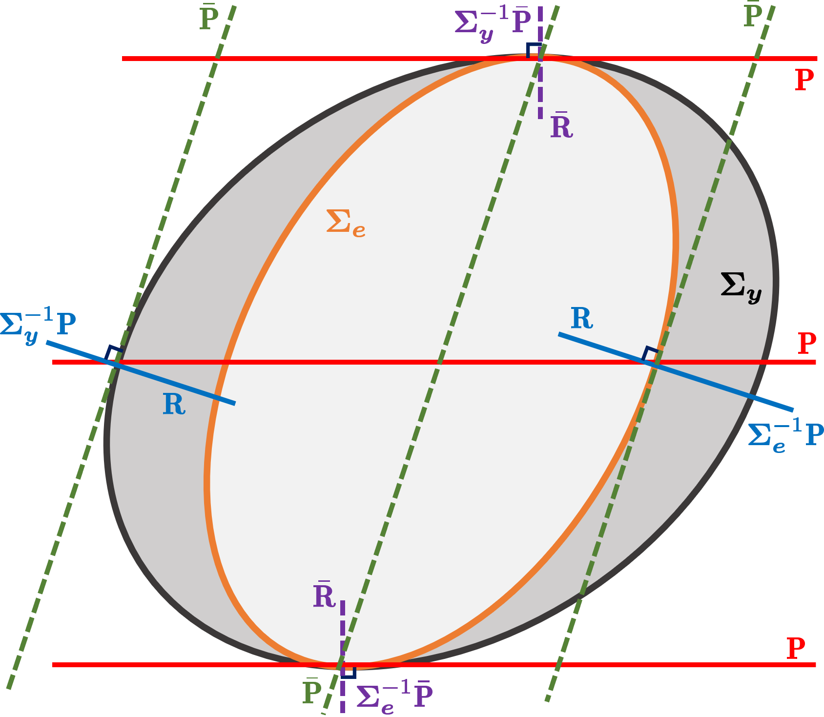
We illustrate the oblique projection necessitated by the covariance of the measurement vector 𝒚k\bm{y}_{k} in Figs. 2(a) and 2(b). Fig. 2(a) gives the oblique geometry of the optimal dynamic-static decomposition for the case of non-singular 𝚺𝒚\mathbf{\Sigma}_{\bm{y}} and 𝚺𝒆\mathbf{\Sigma}_{\bm{e}}, which are respectively represented by the ellipsoids

{𝒙𝒙𝚺𝒚1𝒙1} and {𝒙𝒙𝚺𝒆1𝒙1}.\left\{\bm{x}\mid\bm{x}^{\intercal}\mathbf{\Sigma}_{\bm{y}}^{-1}\bm{x}\leq 1\right\}\text{ and }\left\{\bm{x}\mid\bm{x}^{\intercal}\mathbf{\Sigma}_{\bm{e}}^{-1}\bm{x}\leq 1\right\}.

The two opposite tangent points of the ellipses indicate the static variance direction, which is irreducible by the RRVAR model prediction. The tangent spaces of the two ellipsoids at their intersections on surfaces are the same, agreeing with the range of 𝐏\mathbf{P}. For the best predictability of DLVs in terms of 𝚺𝜺\mathbf{\Sigma}_{\bm{\varepsilon}}, a complementary subspace is chosen such that the oblique projection of the 𝚺𝒆\mathbf{\Sigma}_{\bm{e}}-ellipsoid onto the dynamic subspace along the complementary subspace is as small as possible. Then, the complementary subspace should be specified by the tangent space to the 𝚺𝒆\mathbf{\Sigma}_{\bm{e}}-ellipsoid at the intersection of the dynamic subspace passing the center and the surface. The corresponding normal space is the range of 𝚺𝒆1𝐏\mathbf{\Sigma}_{\bm{e}}^{-1}\mathbf{P}, as shown in Fig. 2(a). Both 𝚺𝒆1𝐏\mathbf{\Sigma}_{\bm{e}}^{-1}\mathbf{P} and 𝐑\mathbf{R} are orthogonal to 𝐏¯\mathbf{\bar{P}}, aligning with Statement (5) in Theorem 2. Similarly, both 𝚺𝒆𝐑¯\mathbf{\Sigma}_{\bm{e}}\mathbf{\bar{R}} and 𝐏¯\mathbf{\bar{P}} are orthogonal to 𝐑\mathbf{R}, agreeing with Statement (4) in Theorem 2.

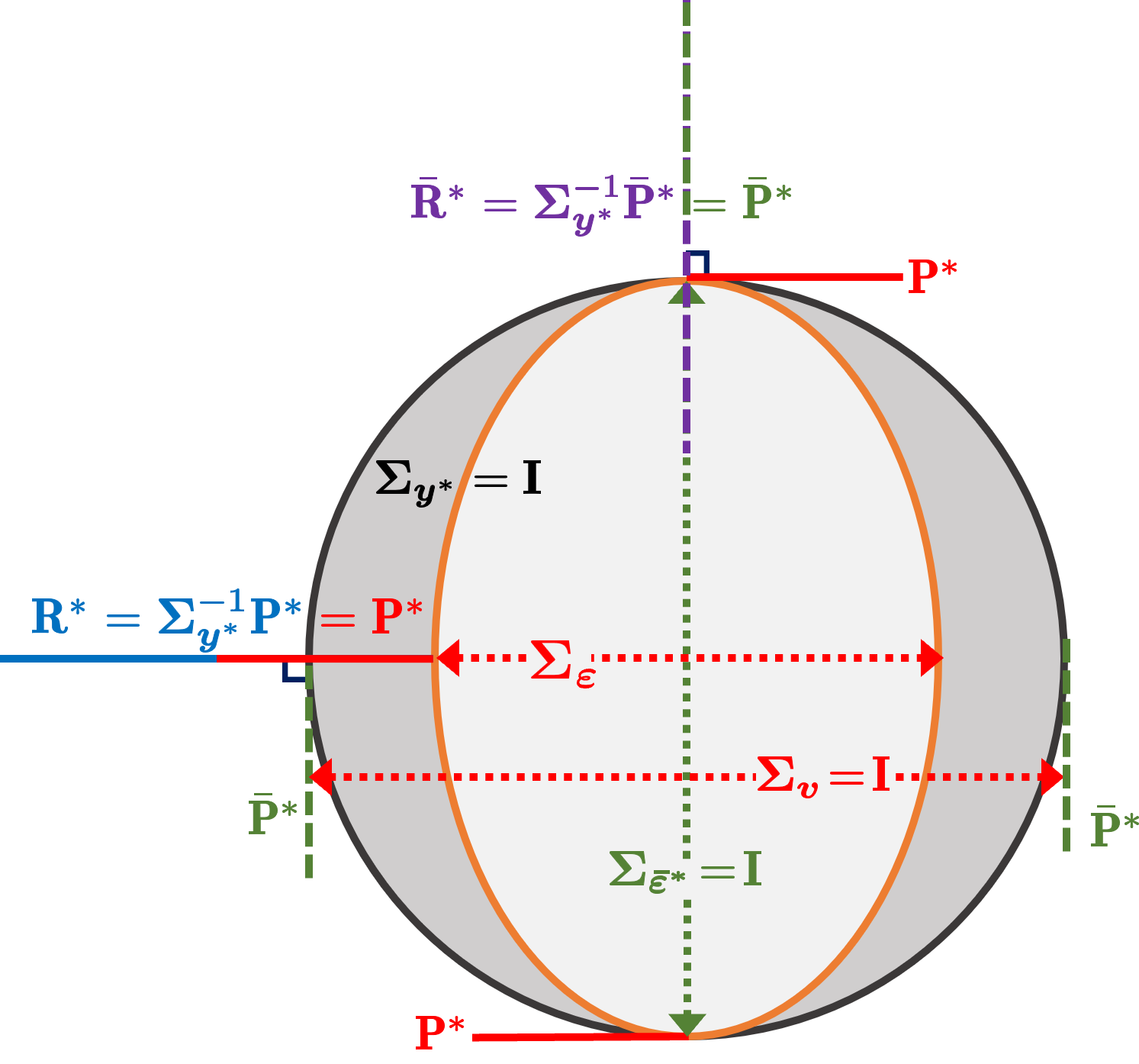
On the other hand, Fig. 2(b) illustrates the orthogonal geometry after normalization with 𝚺𝒚=𝐈\mathbf{\Sigma}_{\bm{y}^{*}}=\mathbf{I}. In this case, the optimal projection is normalized to an orthogonal one, making 𝐑\mathbf{R}^{*} coincide with 𝐏\mathbf{P}^{*}. The covariances for the DLVs and static noise, 𝚺𝒗\mathbf{\Sigma}_{\bm{v}} and 𝚺𝜺¯\mathbf{\Sigma}_{\bm{\bar{\varepsilon}}^{*}}, are scaled to identity matrices. Correspondingly, the predictability of the DLVs is visualized by the volume ratio of the two ellipsoids.

5 Additional Analysis

5.1 Distributions of Parameter Estimates

As in [32], we derive the statistical properties of the model estimates under the assumption that the matrix 𝕍\mathbb{V} of DLVs is fixed. First, it follows that

E(𝔹^𝕍)\displaystyle E(\mathbb{\hat{B}}\mid\mathbb{V}) =E((𝕍𝕍)1𝕍𝐕s𝕍)\displaystyle=E(({\mathbb{V}}^{\intercal}{\mathbb{V}})^{-1}{\mathbb{V}}^{\intercal}\mathbf{V}_{s}\mid\mathbb{V})
=E((𝕍𝕍)1𝕍(𝕍𝔹+𝐄s𝜺)𝕍)=𝔹,\displaystyle=E(({\mathbb{V}}^{\intercal}{\mathbb{V}})^{-1}{\mathbb{V}}^{\intercal}(\mathbb{V}\mathbb{B}+\mathbf{E}^{\bm{\varepsilon}}_{s})\mid\mathbb{V})=\mathbb{B},

and

Var(vec(𝔹^)𝕍)=Var(((𝕍𝕍)1𝕍𝐈)vec(𝐕s)𝕍)\displaystyle\textrm{Var}(\textrm{vec}(\mathbb{\hat{B}}^{\intercal})\mid\mathbb{V})=\textrm{Var}((({\mathbb{V}}^{\intercal}{\mathbb{V}})^{-1}{\mathbb{V}}^{\intercal}\otimes\mathbf{I})\textrm{vec}(\mathbf{V}_{s}^{\intercal})\mid\mathbb{V})
=\displaystyle= Var(((𝕍𝕍)1𝕍𝐈)vec(𝐄s𝜺))𝕍)\displaystyle\textrm{Var}((({\mathbb{V}}^{\intercal}{\mathbb{V}})^{-1}{\mathbb{V}}^{\intercal}\otimes\mathbf{I})\textrm{vec}(\mathbf{E}^{\bm{\varepsilon}^{\intercal}}_{s}))\mid\mathbb{V})
=\displaystyle= E(((𝕍𝕍)1𝕍𝐈)×(𝐈𝚺𝜺)×((𝕍𝕍)1𝕍𝐈)𝕍)\displaystyle E((({\mathbb{V}}^{\intercal}{\mathbb{V}})^{-1}{\mathbb{V}}^{\intercal}\!\otimes\mathbf{I})\!\times\!(\mathbf{I}\otimes\!\mathbf{\Sigma}_{\bm{\varepsilon}})\!\times\!(({\mathbb{V}}^{\intercal}{\mathbb{V}})^{-1}{\mathbb{V}}^{\intercal}\!\otimes\!\mathbf{I})^{\intercal}\mid\mathbb{V})
=\displaystyle= (𝕍𝕍)1𝚺𝜺.\displaystyle({\mathbb{V}}^{\intercal}{\mathbb{V}})^{-1}\otimes\mathbf{\Sigma}_{\bm{\varepsilon}}.

Therefore, 𝔹^\mathbb{\hat{B}} is an unbiased estimate and Var(vec(𝔹^))\textrm{Var}(\textrm{vec}(\mathbb{\hat{B}}^{\intercal})) can be assessed by replacing 𝚺𝜺\mathbf{\Sigma}_{\bm{\varepsilon}} with its estimate.

Similarly, since 𝐄s𝒆=𝐘s𝐕^s𝐏\mathbf{E}^{\bm{e}}_{s}=\mathbf{Y}_{s}-\mathbf{\hat{V}}_{s}\mathbf{P}^{\intercal} is uncorrelated to 𝐕^s\mathbf{\hat{V}}_{s}, it follows from (21) that

E(𝐏^𝕍)\displaystyle E(\mathbf{\hat{P}}\mid\mathbb{V}) =E((𝐄s𝒆+𝐕^s𝐏)𝐕^s(𝐕^s𝐕^s)1𝕍)=𝐏,\displaystyle=E((\mathbf{E}^{\bm{e}}_{s}+\mathbf{\hat{V}}_{s}\mathbf{P}^{\intercal})^{\intercal}\mathbf{\hat{V}}_{s}(\mathbf{\hat{V}}_{s}^{\intercal}\mathbf{\hat{V}}_{s})^{-1}\mid\mathbb{V})=\mathbf{P},

and

Var(vec(𝐏^)𝕍)\displaystyle\textrm{Var}(\textrm{vec}(\mathbf{\hat{P}})\mid\mathbb{V}) =E((𝐕^s𝐕^s)1𝚺𝒆𝕍)\displaystyle=E((\mathbf{\hat{V}}_{s}^{\intercal}\mathbf{\hat{V}}_{s})^{-1}\otimes\mathbf{\Sigma}_{\bm{e}}\mid\mathbb{V})
=(𝔹𝕍𝕍𝔹)1𝚺𝒆.\displaystyle=(\mathbb{B}^{\intercal}\mathbb{V}^{\intercal}\mathbb{V}\mathbb{B})^{-1}\otimes\mathbf{\Sigma}_{\bm{e}}.

Again, 𝚺𝒆\mathbf{\Sigma}_{\bm{e}} can be replaced by its estimate to assess Var(vec(𝐏^))\textrm{Var}(\textrm{vec}(\mathbf{\hat{P}})). To sum up, we conclude that the parameter estimates can be approximated with the following distributions given 𝕍\mathbb{V}:

vec(𝔹^)𝒩(vec(𝔹),(𝕍𝕍)1𝚺^𝜺) and\displaystyle\textrm{vec}(\mathbb{\hat{B}^{\intercal}})\sim{\mathcal{N}}(\textrm{vec}(\mathbb{B}^{\intercal}),({\mathbb{V}}^{\intercal}{\mathbb{V}})^{-1}\otimes\mathbf{\hat{\Sigma}}_{\bm{\varepsilon}})\text{ and }
vec(𝐏^)𝒩(vec(𝐏),(𝔹𝕍𝕍𝔹)1𝚺^𝒆).\displaystyle\textrm{vec}(\mathbf{\hat{P}})\sim{\mathcal{N}}(\textrm{vec}(\mathbf{P}),(\mathbb{B}^{\intercal}\mathbb{V}^{\intercal}\mathbb{V}\mathbb{B})^{-1}\otimes\mathbf{\hat{\Sigma}}_{\bm{e}}).

5.2 Selection of Model Sizes

For full-rank VAR models, the multiple final prediction error (MFPE) developed by Akaike [1] can be used to determine the order ss. Following this idea, we derive a reduced-rank MFPE (RRMFPE) to determine ss and \ell for the RRVAR model. We choose to work on the normalized vector 𝒚k\bm{y}_{k}^{*} since 𝐏\mathbf{P}^{*} and 𝐑\mathbf{R}^{*} coincide with each other and 𝐏\mathbf{P}^{*} and 𝐏¯\mathbf{\bar{P}}^{*} are orthogonal. Therefore, we can write the model explicitly conditional on 𝐏^\mathbf{\hat{P}}^{*} as follows based on (27)

𝒚k|𝐏^=[𝐏^𝐏¯^][j=1s𝐁j|𝐏^𝒗kj|𝐏^+𝜺k|𝐏^𝜺¯k|𝐏^]\displaystyle\bm{y}_{k|\mathbf{\hat{P}}^{*}}^{*}=\begin{bmatrix}\mathbf{\hat{P}}^{*}&\mathbf{\hat{\bar{P}}^{*}}\end{bmatrix}\begin{bmatrix}\sum_{j=1}^{s}\mathbf{B}_{j|\mathbf{\hat{P}}^{*}}\bm{v}_{k-j|\mathbf{\hat{P}}^{*}}+\bm{\varepsilon}_{k|\mathbf{\hat{P}}^{*}}\\ \bm{\bar{\varepsilon}}_{k|\mathbf{\hat{P}^{*}}}^{*}\end{bmatrix}

and the prediction error based on the estimates {𝐁^j|𝐏^}\{{\mathbf{\hat{B}}_{j|\mathbf{\hat{P}}^{*}}}\} is given as follows

𝒚~k|𝐏^=𝒚k|𝐏^𝒚^k|𝐏^\displaystyle\bm{\tilde{y}}_{k|\mathbf{\hat{P}}^{*}}^{*}=\bm{y}_{k|\mathbf{\hat{P}}^{*}}^{*}-\bm{\hat{y}}_{k|\mathbf{\hat{P}}^{*}}^{*}
=\displaystyle= [𝐏^𝐏¯^][j=1s(𝐁j|𝐏^𝐁^j|𝐏^)𝒗kj|𝐏^+𝜺k|𝐏^𝜺¯k|𝐏^].\displaystyle\begin{bmatrix}\mathbf{\hat{P}}^{*}&\mathbf{\hat{\bar{P}}^{*}}\end{bmatrix}\begin{bmatrix}\sum_{j=1}^{s}(\mathbf{B}_{j|\mathbf{\hat{P}}^{*}}-\mathbf{\hat{B}}_{j|\mathbf{\hat{P}}^{*}})\bm{v}_{k-j|\mathbf{\hat{P}}^{*}}+\bm{\varepsilon}_{k|\mathbf{\hat{P}}^{*}}\\ \bm{\bar{\varepsilon}}_{k|\mathbf{\hat{P}^{*}}}^{*}\end{bmatrix}.

The covariance of the prediction error is

E(𝒚~k|𝐏^𝒚~k|𝐏^)=[𝐏^𝐏¯^][𝚺^𝜺+i,j=1sΔ𝐁i|𝐏^𝒗ki|𝐏^𝒗kj|𝐏^Δ𝐁j|𝐏^𝚺^𝜺,𝜺¯𝚺^𝜺¯,𝜺𝚺^𝜺¯][𝐏^𝐏¯^],E\left(\bm{\tilde{y}}_{k|\mathbf{\hat{P}}^{*}}^{*}\bm{\tilde{y}}_{k|\mathbf{\hat{P}}^{*}}^{*\intercal}\right)=\begin{bmatrix}\mathbf{\hat{P}}^{*}&\mathbf{\hat{\bar{P}}^{*}}\end{bmatrix}\\ \begin{bmatrix}\mathbf{\hat{\Sigma}}_{\bm{\varepsilon}}+\!\!\!\sum\limits_{i,j=1}^{s}\!\!\!\mathit{\Delta}\mathbf{B}_{i|\mathbf{\hat{P}}^{*}}\bm{v}_{k-i|\mathbf{\hat{P}}^{*}}\bm{v}_{k-j|\mathbf{\hat{P}}^{*}}^{\intercal}\!\mathit{\Delta}\mathbf{B}_{j|\mathbf{\hat{P}}^{*}}^{\intercal}&\mathbf{\hat{\Sigma}}_{\bm{\varepsilon},\bm{\bar{\varepsilon}}^{*}}\\ \mathbf{\hat{\Sigma}}_{\bm{\bar{\varepsilon}}^{*},\bm{\varepsilon}}&\mathbf{\hat{\Sigma}}_{\bm{\bar{\varepsilon}}^{*}}\end{bmatrix}\begin{bmatrix}\mathbf{\hat{P}}^{*\intercal}\\ \mathbf{\hat{\bar{P}}^{*\intercal}}\end{bmatrix},

where Δ𝐁i|𝐏^=𝐁i|𝐏^𝐁^i|𝐏^\mathit{\Delta}\mathbf{B}_{i|\mathbf{\hat{P}}^{*}}=\mathbf{B}_{i|\mathbf{\hat{P}}^{*}}-\mathbf{\hat{B}}_{i|\mathbf{\hat{P}}^{*}} and 𝚺^𝜺,𝜺¯=𝟎\mathbf{\hat{\Sigma}}_{\bm{\varepsilon},\bm{\bar{\varepsilon}}^{*}}=\mathbf{0} for the PredVAR algorithm. Following [1] and using the fact that 𝐁^j|𝐏^\mathbf{\hat{B}}_{j|\mathbf{\hat{P}}^{*}} from (19) is a least-square estimate with respect to {𝒗k|𝐏^}\{\bm{v}_{k|\mathbf{\hat{P}}^{*}}\}, the estimate of the above covariance is

E^(𝒚~k|𝐏^𝒚~k|𝐏^)=[𝐏^𝐏¯^][1+s/N1s/N𝚺^𝜺𝟎𝟎𝚺^𝜺¯][𝐏^𝐏¯^].{\hat{E}}\left(\bm{\tilde{y}}_{k|\mathbf{\hat{P}}^{*}}^{*}\bm{\tilde{y}}_{k|\mathbf{\hat{P}}^{*}}^{*\intercal}\right)=\begin{bmatrix}\mathbf{\hat{P}}^{*}&\mathbf{\hat{\bar{P}}^{*}}\end{bmatrix}\begin{bmatrix}\frac{1+s\ell/N}{1-s\ell/N}\mathbf{\hat{\Sigma}}_{\bm{\varepsilon}}&\mathbf{0}\\ \mathbf{0}&\mathbf{\hat{\Sigma}}_{\bm{\bar{\varepsilon}}^{*}}\end{bmatrix}\begin{bmatrix}\mathbf{\hat{P}}^{*\intercal}\\ \mathbf{\hat{\bar{P}}^{*\intercal}}\end{bmatrix}.

Since [𝐏^𝐏¯^][𝐏^𝐏¯^]=𝐈\begin{bmatrix}\mathbf{\hat{P}}^{*}&\mathbf{\hat{\bar{P}}^{*}}\end{bmatrix}^{\intercal}\begin{bmatrix}\mathbf{\hat{P}}^{*}&\mathbf{\hat{\bar{P}}^{*}}\end{bmatrix}=\mathbf{I}, taking the determinant of the above covariance estimate gives the RRMFPE of the PredVAR algorithm with the model size (,s)(\ell,s) as follows

RRMFPE(,s)\displaystyle\texttt{RRMFPE}(\ell,s) =det[1+s/N1s/N𝚺^𝜺𝟎𝟎𝚺^𝜺¯]\displaystyle=\textrm{det}\begin{bmatrix}\frac{1+s\ell/N}{1-s\ell/N}\mathbf{\hat{\Sigma}}_{\bm{\varepsilon}}&\mathbf{0}\\ \mathbf{0}&\mathbf{\hat{\Sigma}}_{\bm{\bar{\varepsilon}}^{*}}\end{bmatrix}
=(1+s/N1s/N)det(𝚺^𝜺)det(𝚺^𝜺¯)\displaystyle=\left(\frac{1+s\ell/N}{1-s\ell/N}\right)^{\ell}\textrm{det}(\mathbf{\hat{\Sigma}}_{{\bm{\varepsilon}}})\textrm{det}(\mathbf{\hat{\Sigma}}_{\bm{\bar{\varepsilon}}^{*}})
=(1+s/N1s/N)Πi=1(1λi),\displaystyle=\left(\frac{1+s\ell/N}{1-s\ell/N}\right)^{\ell}\Pi_{i=1}^{\ell}(1-\lambda_{i}), (41)

using 𝚺^𝜺¯=𝐈\mathbf{\hat{\Sigma}}_{\bm{\bar{\varepsilon}}^{*}}=\mathbf{I} and det(𝚺^𝜺)=Πi=1(1λi)\textrm{det}(\mathbf{\hat{\Sigma}}_{{\bm{\varepsilon}}})=\Pi_{i=1}^{\ell}(1-\lambda_{i}) from (34). To handle the possible rank-deficient 𝚺^𝜺\mathbf{\hat{\Sigma}}_{{\bm{\varepsilon}}} due to perfect prediction of some DLVs, denote 𝒮+={i1λi>0, for i=1,,}{\mathcal{S}}_{+}=\{i\mid 1-\lambda_{i}>0,\text{ for }i=1,\cdots,\ell\} and exclude the zero variance terms by replacing det(𝚺^𝜺)\textrm{det}(\mathbf{\hat{\Sigma}}_{{\bm{\varepsilon}}}) with Πi𝒮+(1λi)\Pi_{i\in{\mathcal{S}}_{+}}(1-\lambda_{i}). To further simplify the expression, we take logarithm to obtain

log-RRMFPE(,s)=log1+s/N1s/N+i𝒮+log(1λi).\displaystyle\texttt{log-RRMFPE}(\ell,s)=\ell\log\frac{1+s\ell/N}{1-s\ell/N}+\sum_{i\in{\mathcal{S}}_{+}}\log(1-\lambda_{i}).

When NN is large enough, taking the first-order Taylor approximation gives

log-RRMFPE(,s)=i𝒮+log(1λi)+2s2N.\displaystyle\texttt{log-RRMFPE}(\ell,s)=\sum_{i\in{\mathcal{S}}_{+}}\log(1-\lambda_{i})+2\frac{s\ell^{2}}{N}. (42)

We can fit the model with a grid of (,s)(\ell,s)-pairs, and the one that gives the minimum log-RRMFPE can be chosen as the optimal model size. The two terms in (42) give a clear trade-off between model complicity and model errors. With fixed \ell, the first term decreases with ss, while the second term increases linearly with ss. On the other hand, with fixed ss, the first term decreases with \ell, while the second term increases quadratically with \ell.

5.3 Comparison among PredVAR, LaVAR-CCA, and DiCCA Algorithms

Since the PredVAR, LaVAR-CCA [29], and DiCCA [8] algorithms all use equivalent normalization of the data, it is convenient to compare them using the normalized data {𝒚k}\{\bm{y}^{*}_{k}\}. LaVAR-CCA [29] essentially updates 𝐑^\mathbf{\hat{R}}^{*} by solving the following optimization problem

max𝐑^𝐑^=𝐈𝐑^(𝐘s𝚷𝕍𝐘s/N)𝐑^\underset{\mathbf{\hat{R}}^{*\intercal}\mathbf{\hat{R}}^{*}=\mathbf{I}}{\max\nolimits_{\prec}}\leavevmode\nobreak\ \leavevmode\nobreak\ \mathbf{\hat{R}}^{*\intercal}\left(\mathbf{Y}_{s}^{*\intercal}\mathbf{\Pi}_{\mathbb{V}}\mathbf{Y}_{s}^{*}/N\right)\mathbf{\hat{R}}^{*}

Comparing to (31), the proposed PredVAR algorithm updates 𝐑^\mathbf{\hat{R}}^{*} by

max𝐑^𝐑^=𝐈𝐑^(𝐘s𝚷𝐕^s𝐘s/N)𝐑^\underset{\mathbf{\hat{R}}^{*\intercal}\mathbf{\hat{R}}^{*}=\mathbf{I}}{\max\nolimits_{\prec}}\leavevmode\nobreak\ \leavevmode\nobreak\ \mathbf{\hat{R}}^{*\intercal}\left(\mathbf{Y}_{s}^{*\intercal}\mathbf{\Pi}_{\mathbf{\hat{V}}_{s}}\mathbf{Y}_{s}^{*}/N\right)\mathbf{\hat{R}}^{*}

Therefore, the two algorithms are different in general. As per (20), the range of 𝐕^s\mathbf{\hat{V}}_{s} is contained in that of 𝕍\mathbb{V}, that is, Span(𝐕^s)Span(𝕍)Span(\mathbf{\hat{V}}_{s})\subseteq Span(\mathbb{V}). A projection onto the former implies a more parsimonious model. Consequently, the PredVAR algorithm focuses on the portion of the past information that is relevant to predicting the current data. Therefore, the PredVAR algorithm makes better use of the latent dynamics for the optimal dimension reduction than LaVAR-CCA. The two algorithms coincide in the special case of s=1s=1 since the range of 𝐕^s\mathbf{\hat{V}}_{s} is the same as that of 𝕍\mathbb{V}.

The difference between PredVAR and DiCCA is evident since DiCCA works on univariate latent dynamics. For the special case of =1\ell=1, DiCCA and LaVAR-CCA use the same objective. However, the difference between PredVAR and DiCCA remains since the range of 𝐕^s\mathbf{\hat{V}}_{s} is contained in that of 𝕍\mathbb{V}.

5.4 Comparison to Non-iterative One-Shot Solutions

The PredVAR, LaVAR-CCA, and DiCCA algorithms are all iterative to find 𝐑^\mathbf{\hat{R}}^{*}. In the literature, papers like [14] adopt non-iterative one-shot (OS) solutions, which do not enforce an explicit latent VAR model to obtain 𝐑^\mathbf{\hat{R}}^{*}. The DLV sequences are calculated and used to retrofit the VAR model matrices similar to (19). However, the estimated VAR model is not used to further update 𝐑^\mathbf{\hat{R}}^{*}. Thus, OS solutions appear to be a single iteration step of the iterative algorithms like the PredVAR.

We consider the OS algorithm developed in [14] and compare it with PredVAR. The work in [14] first normalizes the data and obtains an orthonormal 𝐑¯^\mathbf{\hat{\bar{R}}^{*}} from the eigenvectors corresponding to the least pp-\ell eigenvalues of

k=1s(𝐘s𝐘sk)(𝐘s𝐘sk)=𝐘s𝕐𝕐𝐘s,\displaystyle\sum_{k=1}^{s}(\mathbf{Y}_{s}^{*\intercal}\mathbf{Y}_{s-k}^{*})(\mathbf{Y}_{s}^{*\intercal}\mathbf{Y}_{s-k}^{*})^{\intercal}=\mathbf{Y}_{s}^{*\intercal}\mathbb{Y}^{*}\mathbb{Y}^{*\intercal}\mathbf{Y}_{s}^{*}, (43)

where ss is the same as k0k_{0} in [14] as a pre-specified integer. Using 𝐑¯^\mathbf{\hat{\bar{R}}^{*}} to obtain 𝐑¯^\mathbf{\hat{\bar{R}}}, 𝐑^\mathbf{\hat{R}} is found to be the eigenvectors associated with the \ell smallest eigenvalues of 𝚺^𝒚𝐑¯^𝐑¯^𝚺^𝒚\mathbf{\hat{\Sigma}}_{\bm{y}}\mathbf{\hat{\bar{R}}}\mathbf{\hat{\bar{R}}}^{\intercal}\mathbf{\hat{\Sigma}}_{\bm{y}}. In other words, 𝐑^𝚺^𝒚𝐑¯^𝐑¯^𝚺^𝒚𝐑^\mathbf{\hat{R}}^{\intercal}\mathbf{\hat{\Sigma}}_{\bm{y}}\mathbf{\hat{\bar{R}}}\mathbf{\hat{\bar{R}}}^{\intercal}\mathbf{\hat{\Sigma}}_{\bm{y}}\mathbf{\hat{R}} is a diagonal matrix of the \ell smallest eigenvalues. This solution is consistent with (6) in Theorem 2, which makes 𝐑^𝚺^𝒚𝐑¯^\mathbf{\hat{R}}^{\intercal}\mathbf{\hat{\Sigma}}_{\bm{y}}\mathbf{\hat{\bar{R}}} zero ideally.

It is apparent that the above OS solution resembles the initialization step of PredVAR in (39), but ignores the subsequent iterations of the PredVAR algorithm. The OS solution from (43) finds the left singular vectors of 𝐘s𝕐\mathbf{Y}_{s}^{*\intercal}\mathbb{Y}^{*}, which is essentially the covariance from the two matrices. On the other hand, the initialization step of PredVAR in (39) makes use of the eigenvectors of 𝐘s𝕐(𝕐𝕐)1𝕐𝐘s\mathbf{Y}_{s}^{*\intercal}\mathbb{Y}^{*}(\mathbb{Y}^{*\intercal}\mathbb{Y}^{*})^{-1}\mathbb{Y}^{*\intercal}\mathbf{Y}_{s}^{*}, which are projections of 𝐘s\mathbf{Y}_{s}^{*} onto Span(𝕐)Span(\mathbb{Y}^{*}), or the left singular vectors of 𝐘s𝕐(𝕐𝕐)12\mathbf{Y}_{s}^{*\intercal}\mathbb{Y}^{*}(\mathbb{Y}^{*\intercal}\mathbb{Y}^{*})^{-\frac{1}{2}}. Since the covariance of 𝐘s\mathbf{Y}_{s}^{*} is identity, 𝐘s𝕐(𝕐𝕐)12\mathbf{Y}_{s}^{*\intercal}\mathbb{Y}^{*}(\mathbb{Y}^{*\intercal}\mathbb{Y}^{*})^{-\frac{1}{2}} contains the canonical correlations from the two matrices.

To summarize, one-shot solutions like [14] resemble the initialization step of iterative solutions such as PredVAR and do not iterate further to enforce consistency of the outer projection and inner dynamic VAR models. In addition, [14] relies on the covariance 𝐘s𝕐\mathbf{Y}_{s}^{*\intercal}\mathbb{Y}^{*} instead of the correlations 𝐘s𝕐(𝕐𝕐)12\mathbf{Y}_{s}^{*\intercal}\mathbb{Y}^{*}(\mathbb{Y}^{*\intercal}\mathbb{Y}^{*})^{-\frac{1}{2}} to find the solution. The difference between the two is the weight matrix (𝕐𝕐)12(\mathbb{Y}^{*\intercal}\mathbb{Y}^{*})^{-\frac{1}{2}}, whose effect has been studied in the subspace identification literature extensively [23, 20, 6]. It is noted that the weight matrix does affect the singular vector solutions.

6 Case Studies

In this section, we conduct comprehensive numerical comparisons of the proposed PredVAR algorithm with other leading algorithms, including the LaVAR-CCA (abbreviated as LaVAR) in [29], DiCCA in [8], and the one-shot algorithm in [14] (see Sec. 5.4). All simulations are conducted via MATLAB with an Apple M2 Pro.

?tablename? 2: Performance of PredVAR under different model sizes (,s)(\ell,s).
\ell ss 2 12 22 32 42 52
1 0.8265 0.8198 0.8198 0.8198 0.8198 0.8198
2 0.6032 0.5918 0.5918 0.5918 0.5918 0.5918
3 0.1891 0.1895 0.1895 0.1895 0.1896 0.1895
4 0.5142 0.5132 0.5129 0.5127 0.5126 0.5123
5 0.6385 0.6379 0.6381 0.6386 0.6388 0.6383
6 0.7071 0.7071 0.7071 0.7071 0.7071 0.7071
(a) D-distance between the ranges of 𝐏^\mathbf{\hat{P}} and 𝐏\mathbf{P}.
\ell ss 2 12 22 32 42 52
1 0.3129 0.7641 0.7599 0.7592 0.7589 0.7586
2 0.6349 0.9166 0.9123 0.9119 0.9117 0.9117
3 0.9995 0.9995 0.9995 0.9995 0.9995 0.9995
4 0.7658 0.7543 0.7599 0.7714 0.7670 0.7716
5 0.6995 0.7086 0.7002 0.7242 0.7489 0.6853
6 0.6501 0.6501 0.6501 0.6501 0.6501 0.6501
(b) Average correlation between {𝐏^𝒗k|𝐑^}\{\mathbf{\hat{P}}\bm{v}_{k|\mathbf{\hat{R}}}\} and {𝐏𝒗k}\{\mathbf{P}\bm{v}_{k}\}.
\ell ss 2 12 22 32 42 52
1 0.3112 0.7641 0.7599 0.7590 0.7583 0.7573
2 0.6332 0.9166 0.9123 0.9120 0.9120 0.9119
3 0.9974 0.9698 0.9994 0.9994 0.9995 0.9995
4 0.9987 0.9897 0.9870 0.9851 0.9827 0.9806
5 0.9981 0.9869 0.9833 0.9769 0.9781 0.9688
6 0.9977 0.9837 0.9759 0.9680 0.9616 0.9546
(c) Average correlation between {𝐏^𝒗^k|𝐑^}\{\mathbf{\hat{P}}\bm{\hat{{v}}}_{k|\mathbf{\hat{R}}}\} and {𝐏𝒗k}\{\mathbf{P}\bm{v}_{k}\}.
\ell ss 2 12 22 32 42 52
1 0.9993 1.0000 1.0000 1.0000 1.0000 1.0000
2 0.9997 1.0000 1.0000 1.0000 1.0000 1.0000
3 0.9975 0.9680 0.9999 0.9999 0.9999 0.9999
4 0.7657 0.7517 0.7561 0.7678 0.7621 0.7673
5 0.6990 0.7037 0.6937 0.7199 0.7430 0.6718
6 0.6495 0.6436 0.6409 0.6396 0.6348 0.6324
(d) Average correlation between {𝐏^𝒗^k|𝐑^}\{\mathbf{\hat{P}}\bm{\hat{v}}_{k|\mathbf{\hat{R}}}\} and {𝐏^𝒗k|𝐑^}\{\mathbf{\hat{P}}\bm{v}_{k|\mathbf{\hat{R}}}\}.
\ell ss 2 12 22 32 42 52
1 0.1633 0.4891 0.4876 0.4873 0.4872 0.4870
2 0.4127 0.6072 0.6056 0.6055 0.6054 0.6054
3 0.6505 0.6505 0.6505 0.6505 0.6505 0.6505
4 0.8634 0.8763 0.8689 0.8542 0.8583 0.8480
5 0.9424 0.9231 0.9288 0.9094 0.8725 0.9439
6 1.0000 1.0000 1.0000 1.0000 1.0000 1.0000
(e) Average correlation between {𝐏^𝒗k|𝐑^}\{\mathbf{\hat{P}}\bm{v}_{k|\mathbf{\hat{R}}}\} and {𝒚k}\{\bm{y}_{k}\}.
\ell ss 2 12 22 32 42 52
1 0.1623 0.4895 0.4883 0.4888 0.4881 0.4873
2 0.4117 0.6076 0.6063 0.6070 0.6068 0.6066
3 0.6491 0.6305 0.6512 0.6515 0.6514 0.6513
4 0.6503 0.6470 0.6468 0.6474 0.6463 0.6461
5 0.6497 0.6452 0.6437 0.6452 0.6446 0.6380
6 0.6495 0.6436 0.6409 0.6396 0.6348 0.6324
(f) Average correlation between {𝐏^𝒗^k|𝐑^}\{\mathbf{\hat{P}}\bm{\hat{v}}_{k|\mathbf{\hat{R}}}\} and {𝒚k}\{\bm{y}_{k}\}.

6.1 Case Study with the Lorenz Attractor Data

As in [29], use the nonlinear Lorenz oscillator to generate 10,00010,000 samples for the DLV {𝒗k3}\{\bm{v}_{k}\in\Re^{3}\}. The static noise {𝜺¯k3}\{\bm{\bar{\varepsilon}}_{k}\in\Re^{3}\} is generated following a zero-mean Gaussian distribution whose variance is the same as that of the DLV series. Then, the 66-dimensional measurement samples {𝒚k}\{\bm{y}_{k}\} is obtained by mixing the DLVs and static noise via (1), where 𝐏,𝐏¯6×3\mathbf{P},\mathbf{\bar{P}}\in\Re^{6\times 3} are orthonormal and [𝐏𝐏¯][\mathbf{P}\leavevmode\nobreak\ \leavevmode\nobreak\ \mathbf{\bar{P}}] is invertible. The first 7,0007,000 measurement samples are for training, and the remaining is for testing.

Refer to caption
(a) D-distance between the ranges of 𝐏^\mathbf{\hat{P}} and 𝐏\mathbf{P}.
Refer to caption
(b) Average correlation between {𝐏^𝒗k|𝐑^}\{\mathbf{\hat{P}}\bm{v}_{k|\mathbf{\hat{R}}}\} and {𝐏𝒗k}\{\mathbf{P}\bm{v}_{k}\}.
Refer to caption
(c) Average correlation between {𝐏^𝒗^k|𝐑^}\{\mathbf{\hat{P}}\bm{\hat{v}}_{k|\mathbf{\hat{R}}}\} and {𝐏𝒗k}\{\mathbf{P}\bm{v}_{k}\}.
Refer to caption
(d) Average correlation between {𝐏^𝒗^k|𝐑^}\{\mathbf{\hat{P}}\bm{\hat{v}}_{k|\mathbf{\hat{R}}}\} and {𝐏^𝒗k|𝐑^}\{\mathbf{\hat{P}}\bm{v}_{k|\mathbf{\hat{R}}}\}.
?figurename? 3: Performance of PredVAR, LaVAR-CCA, DiCCA, and OS over multiple measurement time series.
Refer to caption
?figurename? 4: Training time of various algorithms
?tablename? 3: D-distance between the ranges of 𝐏^\mathbf{\hat{P}} estimated by PredVAR, LaVAR-CCA, and DiCCA as ss or \ell varies.
ss (with =14\ell=14) 1 2 3 4 5 6 7 8 9 10 11 12
PredVAR – LaVAR 0.0001 0.0001 0.0000 0.0000 0.0001 0.0002 0.0000 0.0000 0.0000 0.0000 0.0002 0.0000
PredVAR – DiCCA 0.0539 0.0297 0.0480 0.0320 0.0308 0.0392 0.0440 0.0378 0.0401 0.0486 0.0515 0.0518
LaVAR – DiCCA 0.0539 0.0297 0.0480 0.0320 0.0308 0.0393 0.0440 0.0378 0.0401 0.0486 0.0514 0.0518
\ell (with s=5s=5) 6 7 8 9 10 11 12 13 14 15 16 17
PredVAR – LaVAR 0.1494 0.1203 0.3430 0.3234 0.0078 0.0004 0.0005 0.0008 0.0000 0.0008 0.0002 0.0045
PredVAR – DiCCA 0.4287 0.4055 0.2977 0.1990 0.2037 0.0961 0.1283 0.0538 0.0518 0.1146 0.2427 0.1350
LaVAR – DiCCA 0.4104 0.3949 0.2284 0.3392 0.2009 0.0960 0.1285 0.0541 0.0518 0.1151 0.2427 0.1314

6.1.1 The DLD \ell and the VAR order ss

Given the estimated model sizes (,s)(\ell,s), we first identify the PredVAR parameters via the proposed algorithm using the training data and then validate the performance of the estimated model using the testing data. To compare between two loadings matrices 𝐏1p×l1\mathbf{P}_{1}\in\Re^{p\times l_{1}} and 𝐏2p×l2\mathbf{P}_{2}\in\Re^{p\times l_{2}}, the D-distance between them defined in [24, 14] is adopted and extended for the case of l1l2l_{1}\geq l_{2} as follows

1trace(𝐏1(𝐏1𝐏1)1𝐏1𝐏2(𝐏2𝐏2)1𝐏2)/l1.\sqrt{1-\textrm{trace}\left(\mathbf{P}_{1}(\mathbf{P}_{1}^{\intercal}\mathbf{P}_{1})^{-1}\mathbf{P}_{1}^{\intercal}\mathbf{P}_{2}(\mathbf{P}_{2}^{\intercal}\mathbf{P}_{2})^{-1}\mathbf{P}_{2}^{\intercal}\right)/l_{1}}.

We further define the average correlation between {𝒚k}\{\bm{y}_{k}\} and {𝒚k}\{\bm{y}^{\prime}_{k}\} by the average absolute value of the pair-wise correlations, i.e.,

i=1p|corr(yi,yi)|/p.\sum\nolimits_{i=1}^{p}|\text{corr}(y_{i},y^{\prime}_{i})|/p.

With the two measures, Table 2 shows the performances of our approach under the different (,s)(\ell,s)-pairs. Since 𝒗k\bm{v}_{k} depends on the latent coordinates from various methods, we map it to the original data space by the loadings matrix 𝐏\mathbf{P} or its estimate 𝐏^\mathbf{\hat{P}} to compare various models.

It is easily seen from Tables 2(a) – 2(d) that =3\ell=3, which is also the truth, gives the highest average correlation between the original noise-free signal series {𝐏𝒗k}\{\mathbf{P}\bm{v}_{k}\} and the signal reconstruction series {𝐏^𝒗k|𝐑^}\{\mathbf{\hat{P}}\bm{v}_{k|\mathbf{\hat{R}}}\} (Table 2(b)) or the signal prediction series {𝐏^𝒗^k|𝐑^}\{\mathbf{\hat{P}}\bm{\hat{v}}_{k|\mathbf{\hat{R}}}\} (Table 2(c)).

Since the noise-free series {𝐏𝒗k}\{\mathbf{P}\bm{v}_{k}\} is unavailable in practical scenarios, Table 2(d) – 2(f) deserves particular attention. Specifically, for each ss, the average correlation between {𝐏^𝒗^k|𝐑^}\{\mathbf{\hat{P}}\bm{\hat{v}}_{k|\mathbf{\hat{R}}}\} and {𝐏^𝒗k|𝐑^}\{\mathbf{\hat{P}}\bm{v}_{k|\mathbf{\hat{R}}}\} significantly deceases as the overestimate of \ell occurs. Moreover, for a proper ss, the average correlation between {𝐏^𝒗^k|𝐑^}\{\mathbf{\hat{P}}\bm{\hat{v}}_{k|\mathbf{\hat{R}}}\} and {𝒚k}\{\bm{y}_{k}\} achieves the maximum value when =3\ell=3.

6.1.2 Comparison to other Methods

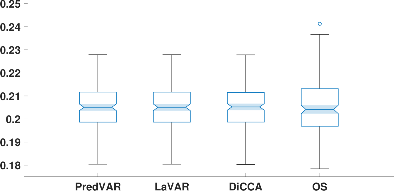
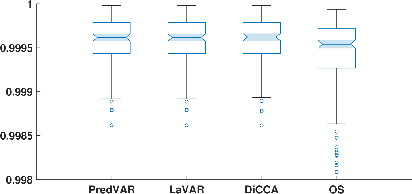
Using the same DLV series and loadings matrices, we perform a Monte-Carlo simulation of the noise from the same distribution to obtain 200200 series of 10,00010,000 points each. For each time series, the first 7,0007,000 data points are for training and the rest for testing. Uniformly set =3\ell=3 and s=2s=2. Fig. 3 shows the performance of the PredVAR and the benchmark algorithms on the testing data series.

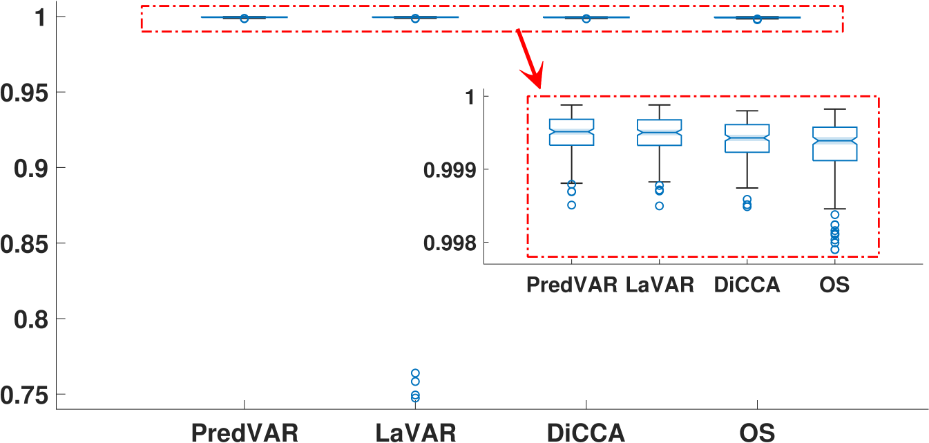
Figs. 3(a) and 3(b) show that the PredVAR, LaVAR, and DiCCA algorithms are comparable in identifying the dynamic subspace and reconstructing the uncorrupted signal. In contrast, the OS algorithm has notably inferior performance. Moreover, the OS algorithm exhibits more significant variability regarding subspace identification and signal reconstruction than the other algorithms.

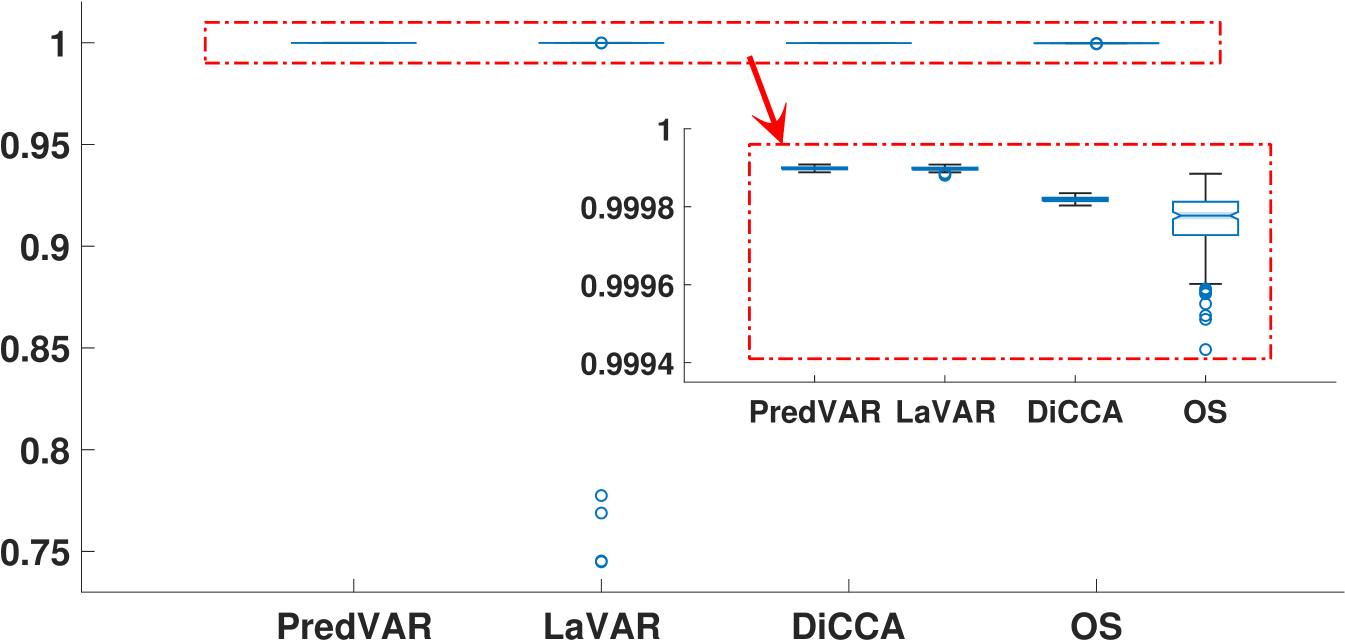
Fig. 3(c) showcases the performance of various algorithms in predicting the noise-free signal, with the PredVAR approach performing the best. In most cases, the LaVAR algorithm performs similarly to PredVAR and surpasses DiCCA and OS. However, LaVAR exhibits more significant outliers than the other three algorithms, meaning that LaVAR is numerically less reliable. A similar phenomenon is observed in Fig. 3(d), regarding the average correlation between the reconstruction and prediction time series. Furthermore, in Fig. 3(d), DiCCA and OS perform significantly worse than PredVAR and LaVAR in general. This fact strongly verifies the importance of exploring the interactions among different DLVs and the alternating updates of projection-related and dynamics-related parameters.

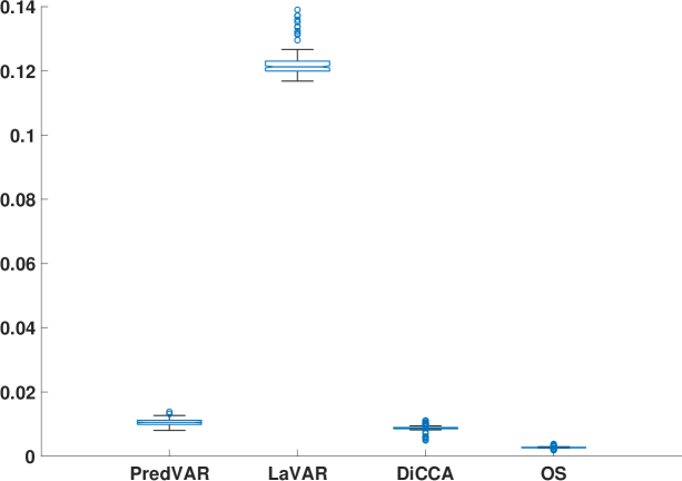
We also compare the algorithms in terms of training time. As shown in Fig. 4, OS requires the least training effort, and LaVAR demands the most. One would expect DiCCA to have less training time than PredVAR and LaVAR since DiCCA does not involve interactions among DLVs. Surprisingly, Fig. 4 suggests that PredVAR takes slightly less training time than DiCCA. However, a unique advantage of DiCCA over other interacting DLV models is that, when a DiCCA model with \ell DLVs is obtained, it yields a suite of DiCCA models for 1:1:\ell. For algorithms with interacting DLV models, one has to build one model with each DLD from 1 to \ell.

6.2 Case Study on Industrial Process Data

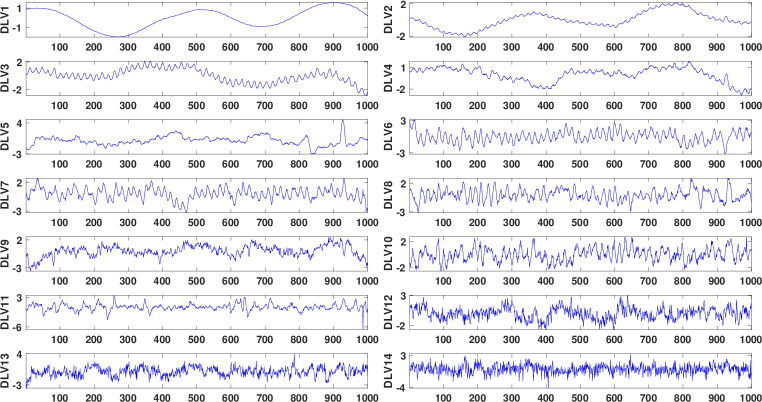
In this study, the plant-wide oscillation dataset from the Eastman Chemical Company [29] is used to demonstrate the effectiveness of the proposed PredVAR algorithm, where 1818 variables with oscillation patterns are selected for modeling over their first 1,0001,000 sequential samples.

The RRMFPE criterion suggests =14\ell=14 and s=5s=5. With such model sizes, the DLVs extracted by the PredVAR algorithm are plotted in Fig. 5. The first three DLVs prominently display low-frequency oscillations. The last DLV seems to exhibit the highest volatility. Moreover, Table 3 depicts the D-distances between the dynamic subspaces estimated by PredVAR, LaVAR-CCA, and DiCCA as ss or \ell varies. Similarly to before, the difference is more responsive to the change of \ell than ss. The dynamic subspaces obtained by PredVAR and LaVAR-CCA are more similar than those estimated by DiCCA.

Refer to caption
?figurename? 5: DLVs extracted by the PredVAR algorithm with =14\ell=14 and s=5s=5 for the Eastman Process Data.

7 Conclusions

A probabilistic reduced dimensional VAR modeling algorithm, namely, PredVAR, is successfully developed with oblique projections, which is required for optimal low-dimensional dynamic modeling from high-dimensional data. The PredVAR model is equivalent to a reduced-rank VAR model, where the VAR coefficient matrices have reduced rank. Both model forms admit a serially independent subspace of the measurement vector. The algorithm is iterative, following the principle of expectation maximization, which alternately estimates the DLV dynamic model and the outer oblique projection. We show with a simulated case and an industrial case study that the PredVAR algorithm with the oblique projections outperforms other recently developed algorithms, including a non-iterative one for reduced-dimensional dynamic modeling. The computational cost of the EM-based PredVAR algorithm is much reduced compared to the alternating optimization based LaVAR algorithm in [29].

?refname?

  • [1] H. Akaike. Autoregressive model fitting for control. Ann. Inst. Stat. Math., 23:163–180, 1971.
  • [2] J. Bai and K. Li. Statistical analysis of factor models of high dimension. Ann. Stat., 40:436–465, 2012.
  • [3] G. E. P. Box and G. C. Tiao. A canonical analysis of multiple time series. Biometrika, 64(2):355–365, 1977.
  • [4] S. Boyd and L. Vandenberghe. Convex Optimization. Cambridge university press, 2004.
  • [5] W. Cao, G. Picci, and A. Lindquist. Identification of low rank vector processes. Automatica, 151:110938, 2023.
  • [6] A. Chiuso and G. Picci. Consistency analysis of some closed-loop subspace identification methods. Automatica, 41:377–391, 2005.
  • [7] A. P. Dempster, N. M. Laird, and D. B. Rubin. Maximum likelihood from incomplete data via the EM algorithm. J. R. Stat. Soc. Ser. B Methodol., 39:1–22, 1977.
  • [8] Y. Dong, Y. Liu, and S. J. Qin. Efficient dynamic latent variable analysis for high-dimensional time series data. IEEE Trans. Ind. Informat., 16(6):4068–4076, 2020.
  • [9] Y. Dong and S. J. Qin. Dynamic latent variable analytics for process operations and control. Comput. Chem. Eng., 114:69–80, 2018.
  • [10] Y. Dong and S. J. Qin. A novel dynamic PCA algorithm for dynamic data modeling and process monitoring. J. Process Control, 67:1–11, 2018.
  • [11] L. Fan, H. Kodamana, and B. Huang. Semi-supervised dynamic latent variable modeling: I/o probabilistic slow feature analysis approach. AIChE J., 65(3), 2019.
  • [12] W. Fan, Q. Zhu, S. Ren, L. Zhang, and F. Si. Dynamic probabilistic predictable feature analysis for multivariate temporal process monitoring. IEEE Trans. Control Syst. Technol., page e17609, 2022.
  • [13] W. D. Fries, X. He, and Y. Choi. LaSDI: Parametric latent space dynamics identification. Comput. Methods Appl. Mech. Eng., 399:115436, 2022.
  • [14] Z. Gao and R. S. Tsay. Modeling high-dimensional time series: A factor model with dynamically dependent factors and diverging eigenvalues. J. Am. Stat. Assoc., pages 1–17, 2021.
  • [15] P. Geladi and B. R. Kowalski. Partial least-squares regression: A tutorial. Anal. Chim. Acta, 185:1–17, 1986.
  • [16] A. J. Izenman. Reduced-rank regression for the multivariate linear model. J. Multivar. Anal., 5(2):248–264, 1975.
  • [17] M. Khosravi and R. S. Smith. The existence and uniqueness of solutions for kernel-based system identification. Automatica, 148:110728, 2023.
  • [18] C. Lam and Q. Yao. Factor modeling for high-dimensional time series: Inference for the number of factors. Ann. Stat., pages 694–726, 2012.
  • [19] G. Li, S. J. Qin, and D. Zhou. A new method of dynamic latent-variable modeling for process monitoring. IEEE Trans. Ind. Electron., 61:6438–6445, 2014.
  • [20] L. Ljung. System Identification: Theory for the User. Prentice-Hall, Inc., Englewood Cliffs, New Jersey, 1999. Second Edition.
  • [21] Z. Lou, Y. Wang, Y. Si, and S. Lu. A novel multivariate statistical process monitoring algorithm: Orthonormal subspace analysis. Automatica, 138:110148, 2022.
  • [22] Y. Mo, J. Yu, and S. J. Qin. Probabilistic reduced-dimensional vector autoregressive modeling for dynamics prediction and reconstruction with oblique projections. In IEEE Conf. Decis. Control (CDC), 2023.
  • [23] P. V. Overschee and B. D. Moor. Subspace Identification for Linear Systems. Kluwer Academic Publishers, 1996.
  • [24] J. Pan and Q. Yao. Modelling multiple time series via common factors. Biometrika, 95(2):365–379, 2008.
  • [25] D. Peña and G. E. P. Box. Identifying a simplifying structure in time series. J. Am. Stat. Assoc., 82:836–843, 1987.
  • [26] D. Peña, E. Smucler, and V. J. Yohai. Forecasting multiple time series with one-sided dynamic principal components. J. Am. Stat. Assoc., 2019.
  • [27] G. Pillonetto, F. Dinuzzo, T. Chen, G. De Nicolao, and L. Ljung. Kernel methods in system identification, machine learning and function estimation: A survey. Automatica, 50:657–682, 2014.
  • [28] S. J. Qin. Latent vector autoregressive modeling for reduced dimensional dynamic feature extraction and prediction. In IEEE Conf. Decis. Control (CDC), pages 3689–3694, 2021.
  • [29] S. J. Qin. Latent vector autoregressive modeling and feature analysis of high dimensional and noisy data from dynamic systems. AIChE J., page e17703, 2022.
  • [30] S. J. Qin, Y. Dong, Q. Zhu, J. Wang, and Q. Liu. Bridging systems theory and data science: A unifying review of dynamic latent variable analytics and process monitoring. Annu Rev Control, 50:29–48, 2020.
  • [31] S. J. Qin, Y. Liu, and S. Tang. Partial least squares, steepest descent, and conjugate gradient for regularized predictive modeling. AIChE J., 69(4):e17992, 2023.
  • [32] G. Reinsel and R. Velu. Multivariate Reduced-Rank Regression, volume 136 of Lecture Notes in Statistics. Springer, New York, NY, 1998.
  • [33] C. Shang, F. Yang, B. Huang, and D. Huang. Recursive slow feature analysis for adaptive monitoring of industrial processes. IEEE Trans. Ind. Electron., 65(11):8895–8905, 2018.
  • [34] J. H. Stock and M. W. Watson. Forecasting using principal components from a large number of predictors. J. Am. Stat. Assoc., 97:1167–1179, 2002.
  • [35] M. Sznaier. Control oriented learning in the era of big data. IEEE Control Syst. Lett., 5:1855–1867, 2020.
  • [36] H. H. Weerts, P. M. Van den Hof, and A. G. Dankers. Prediction error identification of linear dynamic networks with rank-reduced noise. Automatica, 98:256–268, 2018.
  • [37] Q. Wen, Z. Ge, and Z. Song. Data-based linear Gaussian state-space model for dynamic process monitoring. AIChE J., 58(12):3763–3776, 2012.
  • [38] J. Yu and S. J. Qin. Latent state space modeling of high-dimensional time series with a canonical correlation objective. IEEE Control Syst. Lett., 6:3469–3474, 2022.
  • [39] W. Yu, M. Wu, B. Huang, and C. Lu. A generalized probabilistic monitoring model with both random and sequential data. Automatica, 144:110468, 2022.
  • [40] C. Zhao and B. Huang. A full-condition monitoring method for nonstationary dynamic chemical processes with cointegration and slow feature analysis. AIChE J., 64(5):1662–1681, 2018.
  • [41] L. Zhou, G. Li, Z. Song, and S. J. Qin. Autoregressive dynamic latent variable models for process monitoring. IEEE Trans. Control Syst. Technol., 25:366–373, 2016.

?appendixname? A Proof of Theorem 1

Proof of Part 1). From the PredVAR model (1) and (2) it is straightforward to have

𝒚k\displaystyle\bm{y}_{k} =j=1s𝐏𝐁j𝒗kj+𝐏𝜺k+𝐏¯𝜺¯k\displaystyle=\sum_{j=1}^{s}\mathbf{P}\mathbf{B}_{j}\bm{v}_{k-j}+\mathbf{P}\bm{\varepsilon}_{k}+\mathbf{\bar{P}}\bm{\bar{\varepsilon}}_{k}
=j=1s𝐏𝐁j𝐑𝒚kj+𝒆k\displaystyle=\sum_{j=1}^{s}\mathbf{P}\mathbf{B}_{j}\mathbf{R}^{\intercal}\bm{y}_{k-j}+\bm{e}_{k}

with 𝐑𝐏=𝐈\mathbf{R}^{\intercal}\mathbf{P}=\mathbf{I}, where 𝒆k=𝐏𝜺k+𝐏¯𝜺¯k\bm{e}_{k}=\mathbf{P}\bm{\varepsilon}_{k}+\mathbf{\bar{P}}\bm{\bar{\varepsilon}}_{k}. Since 𝜺k\bm{\varepsilon}_{k} and 𝜺¯k\bm{\bar{\varepsilon}}_{k} are i.i.d. Gaussian, 𝒆k𝒩(𝟎,𝚺𝒆)\bm{e}_{k}\sim\mathcal{N}(\bm{0},\mathbf{\Sigma}_{\bm{e}}) is i.i.d. Gaussian.

From the canonical RRVAR model, pre-multiplying 𝐑\mathbf{R}^{\intercal} to (8) leads to

𝐑𝒚k\displaystyle\mathbf{R}^{\intercal}\bm{y}_{k} =j=1s𝐑𝐏𝐁j𝐑𝒚kj+𝐑𝒆k\displaystyle=\sum_{j=1}^{s}\mathbf{R}^{\intercal}\mathbf{P}\mathbf{B}_{j}\mathbf{R}^{\intercal}\bm{y}_{k-j}+\mathbf{R}^{\intercal}\bm{e}_{k}
𝒗k\displaystyle\bm{v}_{k} =j=1s𝐏𝐁j𝒗kj+𝜺k,\displaystyle=\sum_{j=1}^{s}\mathbf{P}\mathbf{B}_{j}\bm{v}_{k-j}+\bm{\varepsilon}_{k},

where 𝒗k=𝐑𝒚k\bm{v}_{k}=\mathbf{R}^{\intercal}\bm{y}_{k} and 𝜺k=𝐑𝒆k\bm{\varepsilon}_{k}=\mathbf{R}^{\intercal}\bm{e}_{k}. Since 𝒆k\bm{e}_{k} is i.i.d. Gaussian, 𝜺k𝒩(𝟎,𝐑𝚺𝒆𝐑)\bm{\varepsilon}_{k}\sim\mathcal{N}(\bm{0},\mathbf{R}^{\intercal}\mathbf{\Sigma}_{\bm{e}}\mathbf{R}) is i.i.d. Gaussian.

Let 𝐑¯p×(p)\mathbf{\bar{R}}\in\Re^{p\times(p-\ell)} be an arbitrary matrix that is of full column rank and 𝐑¯𝐏=𝟎\mathbf{\bar{R}}^{\intercal}\mathbf{P}=\bm{0}. It follows that 𝜺¯k=𝐑¯𝒚k=𝐑¯𝒆k\bm{\bar{\varepsilon}}_{k}=\mathbf{\bar{R}}^{\intercal}\bm{y}_{k}=\mathbf{\bar{R}}^{\intercal}\bm{e}_{k}. Since 𝒆k\bm{e}_{k} is i.i.d. Gaussian, 𝜺¯k𝒩(𝟎,𝐑¯𝚺𝒆𝐑¯)\bm{\bar{\varepsilon}}_{k}\sim\mathcal{N}(\bm{0},\mathbf{\bar{R}}^{\intercal}\mathbf{\Sigma}_{\bm{e}}\mathbf{\bar{R}}) is i.i.d. Gaussian. By (3), obtain 𝐏¯\mathbf{\bar{P}} by

𝐏¯=[𝐑𝐑¯]1[𝟎𝐈],\mathbf{\bar{P}}=\begin{bmatrix}\mathbf{R}^{\intercal}\\ \mathbf{\bar{R}}^{\intercal}\end{bmatrix}^{-1}\begin{bmatrix}\bm{0}\\ \mathbf{I}\end{bmatrix},

and it holds that

𝒚k=𝐏𝐑𝒚k+𝐏¯𝐑¯𝒚k=𝐏𝒗k+𝐏¯𝜺¯k.\bm{y}_{k}=\mathbf{P}\mathbf{R}^{\intercal}\bm{y}_{k}+\mathbf{\bar{P}}\mathbf{\bar{R}}^{\intercal}\bm{y}_{k}=\mathbf{P}\bm{v}_{k}+\mathbf{\bar{P}}\bm{\bar{\varepsilon}}_{k}.

Thus, the canonical RRVAR model is equivalently transformed into the PredVAR model (1) and (2).

Proof of Part 2). From (7) we have

𝒚k\displaystyle\bm{y}_{k} =j=1s𝐏´𝐁´j𝐑´𝒚kj+𝒆k\displaystyle=\sum_{j=1}^{s}\mathbf{\acute{P}}\mathbf{\acute{B}}_{j}\mathbf{\acute{R}}^{\intercal}\bm{y}_{k-j}+\bm{e}_{k}
=j=1s𝐏´𝐁´j(𝐑´𝐏´)(𝐑´𝐏´)1𝐑´𝒚kj+𝒆k\displaystyle=\sum_{j=1}^{s}\mathbf{\acute{P}}\mathbf{\acute{B}}_{j}(\mathbf{\acute{R}}^{\intercal}\mathbf{\acute{P}})(\mathbf{\acute{R}}^{\intercal}\mathbf{\acute{P}})^{-1}\mathbf{\acute{R}}^{\intercal}\bm{y}_{k-j}+\bm{e}_{k}
=j=1s𝐏𝐁j𝐑𝒚kj+𝒆k\displaystyle=\sum_{j=1}^{s}\mathbf{P}\mathbf{B}_{j}\mathbf{R}^{\intercal}\bm{y}_{k-j}+\bm{e}_{k}

where 𝐑𝐏=𝐈\mathbf{R}^{\intercal}\mathbf{P}=\mathbf{I} by setting 𝐏=𝐏´\mathbf{P}=\mathbf{\acute{P}}, 𝐁j=𝐁´j𝐑´𝐏´\mathbf{B}_{j}=\mathbf{\acute{B}}_{j}\mathbf{\acute{R}}^{\intercal}\mathbf{\acute{P}}, and 𝐑=𝐑´(𝐏´𝐑´)1\mathbf{R}=\mathbf{\acute{R}}(\mathbf{\acute{P}}^{\intercal}\mathbf{\acute{R}})^{-1}. Further,

𝐑𝐏=(𝐑´𝐏´)1𝐑´𝐏´=𝐈.\mathbf{R}^{\intercal}\mathbf{P}=(\mathbf{\acute{R}}^{\intercal}\mathbf{\acute{P}})^{-1}\mathbf{\acute{R}}^{\intercal}\mathbf{\acute{P}}=\mathbf{I}.

?appendixname? B Proof of Theorem 2

Applying the Lagrangian multiplier 𝚪\mathbf{\Gamma} to (40) leads to

L(𝐑,𝚪)=𝐑𝚺𝒆𝐑+𝚪(𝐈𝐑𝐏)L(\mathbf{R},\mathbf{\Gamma})={\mathbf{R}}^{\intercal}\mathbf{\Sigma}_{\bm{e}}\mathbf{R}+\mathbf{\Gamma}(\mathbf{I}-{\mathbf{R}}^{\intercal}\mathbf{P})

Differentiating LL with respect to 𝐑\mathbf{R} and setting the derivative to zero gives

L𝐑=2𝚺𝒆𝐑𝐏𝚪=𝟎.\frac{\partial L}{\partial\mathbf{R}}=2\mathbf{\Sigma}_{\bm{e}}\mathbf{R}-\mathbf{P}\mathbf{\Gamma}=\bm{0}. (44)

Since 𝐑𝐏=𝐈{\mathbf{R}}^{\intercal}\mathbf{P}=\mathbf{I}, pre-multiplying 𝐑{\mathbf{R}}^{\intercal} to (44) gives

𝚪=2𝐑𝚺𝒆𝐑.\mathbf{\Gamma}=2{\mathbf{R}}^{\intercal}\mathbf{\Sigma}_{\bm{e}}\mathbf{R}. (45)

Substituting (45) into (44) leads to 1). It follows from the Lagrangian multiplier analysis [4] that Problem (40) attains the optimum only if 1) holds. It remains to show the equivalence of the six statements.

1) \Leftrightarrow 2) is due to that 𝐏\mathbf{P} is of full column rank and post-multiplying 𝐏\mathbf{P}^{\intercal} to 1) leads to

(𝐈𝐏𝐑)𝚺𝒆𝐑𝐏=E((𝐈𝐏𝐑)𝒆k𝒆k𝐑𝐏)=𝟎.(\mathbf{I}-\mathbf{P}\mathbf{R}^{\intercal})\mathbf{\Sigma}_{\bm{e}}\mathbf{R}\mathbf{P}^{\intercal}=E\left((\mathbf{I}-\mathbf{P}{\mathbf{R}}^{\intercal}){\bm{e}}_{k}{{\bm{e}}_{k}}^{\intercal}\mathbf{R}{\mathbf{P}}^{\intercal}\right)=\bm{0}.

2) \Leftrightarrow 3) follows from (3), namely

(𝐈𝐏𝐑)𝒆k=𝐏¯𝐑¯𝒆k=𝐏¯𝜺¯k\displaystyle(\mathbf{I}-\mathbf{P}\mathbf{R}^{\intercal})\bm{e}_{k}=\mathbf{\bar{P}}\mathbf{\bar{R}}^{\intercal}\bm{e}_{k}=\mathbf{\bar{P}}\bm{\bar{\varepsilon}}_{k}
𝐑¯((𝐈𝐏𝐑)𝒆k)=𝐑¯𝒆k=𝜺¯k\displaystyle\mathbf{\bar{R}}^{\intercal}((\mathbf{I}-\mathbf{P}\mathbf{R}^{\intercal})\bm{e}_{k})=\mathbf{\bar{R}}^{\intercal}\bm{e}_{k}=\bm{\bar{\varepsilon}}_{k}
𝐑(𝐏𝐑𝒆k)=𝐑𝒆k=𝜺k\displaystyle\mathbf{R}^{\intercal}(\mathbf{P}\mathbf{R}^{\intercal}\bm{e}_{k})=\mathbf{R}^{\intercal}\bm{e}_{k}=\bm{\varepsilon}_{k}

3) \Leftrightarrow 4) follows from the definitions of 𝜺k\bm{\varepsilon}_{k}, 𝜺¯k\bm{\bar{\varepsilon}}_{k}, and 𝚺𝒆\mathbf{\Sigma}_{\bm{e}}.

4) \Leftrightarrow 5) follows from the fact that the inverse of a block diagonal matrix is also block diagonal, and (10).

4) \Leftrightarrow 6) follows from 𝐏𝐑¯=𝟎\mathbf{P}^{\intercal}\mathbf{\bar{R}}=\bm{0} and

𝚺𝒚=𝚺𝒆+𝐏𝚺𝒗^𝐏.\mathbf{\Sigma}_{\bm{y}}=\mathbf{\Sigma}_{\bm{e}}+\mathbf{P}\mathbf{\Sigma}_{\bm{\hat{v}}}\mathbf{P}^{\intercal}.

6) \Leftrightarrow 7) follows from the equivalence among

[𝐑𝐑¯]𝚺𝒚[𝐑𝐑¯]=[𝚺𝒗𝟎𝟎𝚺𝜺¯],\displaystyle\left[\mathbf{R}\leavevmode\nobreak\ \leavevmode\nobreak\ \mathbf{\bar{R}}\right]^{\intercal}\mathbf{\Sigma}_{\bm{y}}\left[\mathbf{R}\leavevmode\nobreak\ \leavevmode\nobreak\ \mathbf{\bar{R}}\right]=\begin{bmatrix}\mathbf{\Sigma}_{\bm{v}}&\bm{0}\\ \bm{0}&\mathbf{\Sigma}_{\bm{\bar{\varepsilon}}}\end{bmatrix},
𝚺𝒚1=[𝐑𝐑¯][𝚺𝒗1𝚺𝜺¯1][𝐑𝐑¯],\mathbf{\Sigma}_{\bm{y}}^{-1}=\left[\mathbf{R}\leavevmode\nobreak\ \leavevmode\nobreak\ \mathbf{\bar{R}}\right]\begin{bmatrix}\mathbf{\Sigma}_{\bm{v}}^{-1}\\ \leavevmode\nobreak\ &\mathbf{\Sigma}_{\bm{\bar{\varepsilon}}}^{-1}\end{bmatrix}\left[\mathbf{R}\leavevmode\nobreak\ \leavevmode\nobreak\ \mathbf{\bar{R}}\right]^{\intercal},

if 𝚺𝒚\mathbf{\Sigma}_{\bm{y}} is non-singular, and

[𝐏𝐏¯]𝚺𝒚1[𝐏𝐏¯]=[𝚺𝒗1𝚺𝜺¯1].\left[\mathbf{P}\leavevmode\nobreak\ \leavevmode\nobreak\ \mathbf{\bar{P}}\right]^{\intercal}\mathbf{\Sigma}_{\bm{y}}^{-1}\left[\mathbf{P}\leavevmode\nobreak\ \leavevmode\nobreak\ \mathbf{\bar{P}}\right]=\begin{bmatrix}\mathbf{\Sigma}_{\bm{v}}^{-1}\\ \leavevmode\nobreak\ &\mathbf{\Sigma}_{\bm{\bar{\varepsilon}}}^{-1}\end{bmatrix}.