Probable brown dwarf companions detected in binary microlensing events during the 2018-2020 seasons of the KMTNet survey
Abstract
Aims. We inspect the microlensing data of the KMTNet survey collected during the 2018–2020 seasons in order to find lensing events produced by binaries with brown-dwarf companions.
Methods. In order to pick out binary-lens events with candidate BD lens companions, we conduct systematic analyses of all anomalous lensing events observed during the seasons. By applying the selection criterion with mass ratio between the lens components of , we identify four binary-lens events with candidate BD companions, including KMT-2018-BLG-0321, KMT-2018-BLG-0885, KMT-2019-BLG-0297, and KMT-2019-BLG-0335. For the individual events, we present the interpretations of the lens systems and measure the observables that can constrain the physical lens parameters.
Results. The masses of the lens companions estimated from the Bayesian analyses based on the measured observables indicate that the probabilities for the lens companions to be in the brown-dwarf mass regime are high: 59%, 68%, 66%, and 66% for the four events respectively.
Key Words.:
gravitational microlensing – (Stars:) brown dwarfs1 Introduction
Due to the trait of occurring by the mass of a lensing object regardless of its luminosity, microlensing provides an important tool to detect very faint and even dark astronomical objects. With this trait, microlensing has been applied to search for extrasolar planets, and about 30 planets are annually being detected (Gould et al., 2022; Jung et al., 2022; Gould, 2022) from the combined observations by survey, for example, the KMTNet (Kim et al., 2016), MOA (Bond et al., 2001), and OGLE (Udalski et al., 2015) experiments, and followup groups, for example, the ROME/REA survey (Tsapras et al., 2019).
Brown dwarfs (BDs) are another population of faint astronomical objects to which microlensing is sensitive. Microlensing BDs can be detected through a single-lens event channel, in which a single BD object produces a lensing event with a short time scale, for example, Han et al. (2020). Considering that BDs may have formed via a similar mechanism to that of stars, BDs can be as abundant as its stellar siblings, and, in this case, a significant fraction of short time-scale lensing events being detected by the surveys may be produced by BDs. Observationally, both radial-velocity (Grether & Lineweaver, 2006) and microlensing (Shvartzvald et al., 2016) studies indicate a deficit of BDs companions compared to both stars and planets, suggesting that microlensing may allows us to study the stars, BDs and planet formation mechanism. However, confirming the BD lens nature of a short time-scale event by measuring the mass of the lens is difficult because the event time scale depends not only on the lens mass but also on the distance to the lens and the relative lens-source proper motion. The lens mass can be determined by simultaneously measuring the extra lensing observables of the angular Einstein radius and microlens parallax , for example, OGLE-2017-BLG-0896 (Shvartzvald et al., 2019), but the fraction of these events is small.
Han et al. (2022), hereafter paper I, investigated the microlensing survey data collected during the early phase of the KMTNet experiment with the aim of finding microlensing binaries containing BD companions. The strategy applied to paper I in finding BD events was picking out lensing events produced by binaries with small companion-to-primary mass ratios , for example, . Considering that typical Galactic lensing events are produced by low-mass stars (Han & Gould, 2003), the companions to the lenses of these events are very likely to be BDs.
Following the work done in Paper I, we report four additional BD binary-lensing events found from the systematic investigation of the 2018–2020 season data of the KMTNet survey. For the use of a future statistical analysis on the properties of BDs based on a uniform sample, we consistently apply the same selection criterion as that applied in paper I in the selection of BD events.
The discoveries and analyses of the BD events are presented according to the following organization. In Sect. 2, we mention the procedure of selecting BD binary-lens events and explain the observations conducted for the selected events. We describe the analysis procedure commonly applied to the lensing events in Sect. 3, and detailed analyses for the individual events are presented in the following subsections. In Sect. 4, we characterize the source stars of the events and estimate their angular Einstein radii. In Sect. 5, we estimate the physical parameters of the lens systems by conducting Bayesian analyses of the events using the measured observables of the individual events. A summary of the results found from the analyses and conclusion are presented in Sect. 6.
2 Event selection and observations
The KMTNet group has conducted a microlensing survey since 2016 by observing stars lying toward the dense Galactic bulge field with the use of three telescopes that are globally distributed in the Southern Hemisphere. For the searches of binary lenses possessing BD companions, we inspect the microlensing data acquired by the KMTNet survey during the three seasons from 2018 to 2020. The survey in the 2020 season was partially conducted because two of the KMTNet telescopes were shutdown due to Covid-19 pandemic for most of that season.
We sort out binary lensing (2L1S) events with candidate BD lens companions by conducting systematic analyses of all anomalous lensing events observed during the seasons. Anomalies induced by planetary companions to the lenses, with companion-to-primary mass ratios of an order of or less, can be, in most cases, readily identified from the characteristic short-term nature of the anomalies (Gould & Loeb, 1992). However, anomalies induced by BD companions, with mass ratios of an order of , usually cannot be treated as perturbations, and thus it is generally much more difficult to distinguish them from those induced by binary lenses with roughly equal-mass components. We, therefore, systematically conducted modelings of all anomalous lensing events detected during the seasons, and then sorted out candidate BD binary-lens events by applying the selection criterion of . The total numbers of lensing events detected by the KMTNet survey are 2781, 3303, and 894 in the 2018, 2019, and 2020 seasons, respectively, and 2L1S events comprise about one tenth of the total events. This fraction of 2L1S events is similar to the one Shvartzvald et al. (2016) found for the OGLE-MOA-Wise sample (12%).
From this procedure, we identified four 2L1S events with candidate BD companions, including KMT-2018-BLG-0321, KMT-2018-BLG-0885, KMT-2019-BLG-0297, and KMT-2019-BLG-0335. We found no BD event among the events detected in the 2020 season not only because the number of detected lensing events during the season is relatively small but also because the data coverage of the individual events was sparse due to the use of a single telescope during the great majority of the season. Among these events, KMT-2019-BLG-0297 was additionally observed by the MOA group, who labeled the event as MOA-2019-BLG-131, and we include their data in the analysis. For this event, we use the KMTNet ID reference following the convention of the microlensing community of using the ID reference of the first discovery survey
The three KMTNet telescopes are identical with a 1.6 m aperture. The sites of the individual telescopes are the Siding Spring Observatory in Australia (KMTA), the Cerro Tololo Interamerican Observatory in Chile (KMTC), and the South African Astronomical Observatory in South Africa (KMTS). The telescope used for the MOA survey has an aperture of 1.8 m and is located at Mt. John Observatory in New Zealand. The fields of view of the cameras installed on the KMTNet and MOA telescopes are 4 deg2 and 2.2 deg2, respectively. Images were primarily taken in the band for the KMTNet survey and in the customized MOA- band for the MOA survey. For both surveys, a minor portion of images were acquired in the band to measure the colors of the source stars. The OGLE survey was conducted during the 2018 and 2019 seasons, but none of the events reported in this work was detected by the OGLE survey.
Reductions of the images and photometry of the events were carried out using the pipelines of the individual survey groups developed by Albrow et al. (2009) for the KMTNet group and Bond et al. (2001) for the MOA group. Following the routine of Yee et al. (2012), we readjust the error bars of each data set estimated by the pipelines in order that the error bars are consistent with the scatter of the data and per degree of freedom (dof) for each data set becomes unity. In the process of readjusting error bars, we use the best-fit model by after rejecting outliers lying beyond a 3 level from the best-fit model. The error-bar normalization is an ever-repeating process because once the error bars are rescaled based on a model obtained at a certain stage, the /dof value can vary in the next modeling run as the model slightly varies from the initial model, and thus the value of /dof can be slightly different from unity. We note that the variation of the lensing parameters caused by the slight change of the /dof value is very minor.
3 Light curve analyses
Under the approximation of a rectilinear relative motion between the lens and source, the light curve of a 2L1S event is characterized by 7 basic lensing parameters. The first three parameters define the lens-source approach, and the individual parameters denote the time of the closest approach, the separation between the lens and source at that time (impact parameter), and the Einstein time scale. The Einstein time scale is defined as the time required for a source to cross the Einstein radius, that is, , where denotes the relative lens-source proper motion. Another three parameters define the binary-lens system, and denotes the projected separation between the lens components with masses and , is the mass ratio, and represents the angle between the direction of and –, axis (source trajectory angle). Here represents the vector of the relative lens-source proper motion. The parameters and are scaled to . The last parameter is defined as the ratio of the angular source radius to , that is, (normalized source radius), and it characterizes the deformation of a lensing light curve by finite-source effects arising when a source crosses or approaches lens caustics.
Caustics represent source positions at which the lensing magnifications of a point source become infinity. Caustics in binary lensing vary depending on the binary parameters and , and their topologies are classified into three categories of “close”, “intermediate”, and “wide” (Schneider & Weiss, 1986; Cassan, 2008). A close binary induces three sets of caustics, in which one lies near the heavier lens component and the other two sets lie on the opposite side of the lighter lens component. On the other hand, a wide binary induces two sets of caustics, which lie close to the individual lens components. In the intermediate regime, the caustics merge together to form a single set of a large caustic.
Besides the basic parameters, detailed modeling of lensing light curves for a fraction of events requires consideration of higher-order effects caused by the deviation of the relative lens-source motion from rectilinear. Such a deviation is induced by two major causes, in which the first is the accelerated motion of an observer caused on the orbital motion of Earth, microlens-parallax effects (Gould, 1992), and the second is the orbital motion of the binary lens, lens-orbital effects, for example, Batista et al. (2011) and Skowron et al. (2011). For the consideration of these higher-order effects, extra parameters are required to be added in modeling. The parameters for the consideration of the microlens-parallax effects are , which represent the north and east components of the microlens-parallax vector , respectively. Here represents the relative parallax of the lens and source. Under the approximation of a minor change of the lens configuration by the orbital motion, the lens-orbital effects are described by two parameters of , which represent the change rates of the binary separation and source trajectory angle, respectively.
The analyses of the events were carried out by finding lensing solutions, representing a set of parameters describing the observed light curves. The searches for the lensing parameters were done in two steps. In the first step, we conducted grid searches for the binary parameters and , and for each pair of the grid parameters and , we found the other parameters using a downhill approach based on the Markov Chain Monte Carlo (MCMC) logic. In this stage, we constructed a map on the plane of the grid parameters and identified local solutions on the map. In the second step, we refined the individual local solutions by allowing all parameters to vary. If a single solution can be distinguished from the other local minima with a significant difference, we provide a single global solution. If the degeneracy between local solutions is severe, by contrast, we present all local solutions with the explanations on the causes of the degeneracy. In the following subsections, we present the analyses of the individual events.
3.1 KMT-2018-BLG-0321
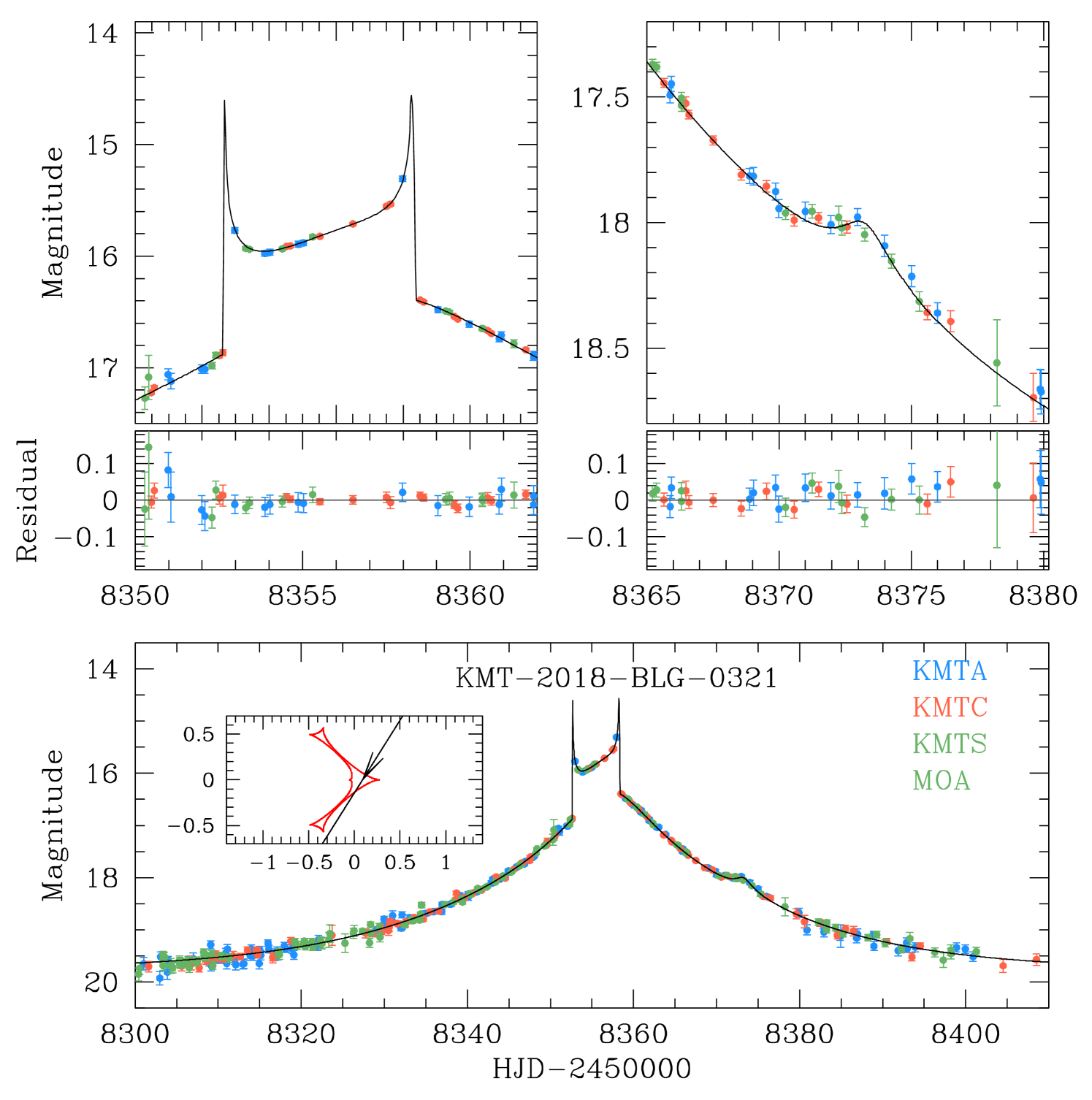
The source of the lensing event KMT-2018-BLG-0321 lies in the Galactic bulge field with Equatorial coordinates (RA, DEC)17:41:36.41, -22:09:52.88), which correspond to the Galactic coordinates . The event was detected by the KMTNet survey on 2018 July 21 (), when the source was brighter by magnitude than the baseline of using the AlertFinder algorithm of the KMTNet survey (Kim et al., 2018b). The source of the event lies in the KMTNet BLG20 field, toward which observations were conducted with a 2.5 hr cadence.
The lensing light curve of KMT-2018-BLG-0321 is presented in Figure 1. It shows that the light curve exhibits deviations from the smooth and symmetric form of a single-lens single-source (1L1S) event. The deviations are characterized by three major anomaly features, including the two spike features appearing around the peak of the light curve at and 8358.2, and the weak bump appearing on the falling side of the light curve at . From their shapes, the two spike features are likely to be produced by the source crossings over folds of a binary caustic, and the bump feature is likely to be generated by the source approach to a cusp of the caustic
| Parameter | Value |
|---|---|
| /dof | |
| (HJD′) | |
| (days) | |
| (rad) | |
| () |
From the detailed modeling of the observed light curve, we found that the event was generated by a binary lens with a small mass ratio between the lens components. We found a unique solution without any degeneracy, and the estimated binary parameters are . The exact values of the lensing parameters are listed in Table 1 together with the value of . Neither of the caustic-crossing features was resolved, and only an upper limit on could be constrained. It was found that secure measurements of the higher-order lensing parameters were difficult due to the moderate time scale, days, of the event.
The inset in the bottom panel of Figure 1 shows the lens system configuration of the event. The caustic is at the boundary between the close and intermediate regimes, and the two peripheral caustics are connected with the central caustic by slim bridges. The best-fit model indicates that the two caustic spikes were produced when the source entered and exited the central caustic, and the weak bump on the falling side of the light curve was produced when the source approached close to one of the two peripheral caustics.
3.2 KMT-2018-BLG-0885
The lensing event KMT-2018-BLG-0885 occurred on a source lying at (RA, DEC)17:55:51.92, -28:30:48.10), . The event occurred before the full operation of the KMTNet AlertFinder system, and it was identified from the inspection of the data after the bulge season was over by the KMTNet EventFinder system (Kim et al., 2018a). The source of the event lies in the two overlapping KMTNet fields of BLG02 and BLG42, each of which was monitored with a 0.5 hr cadence, and thus with a combined cadence of 0.25 hr.
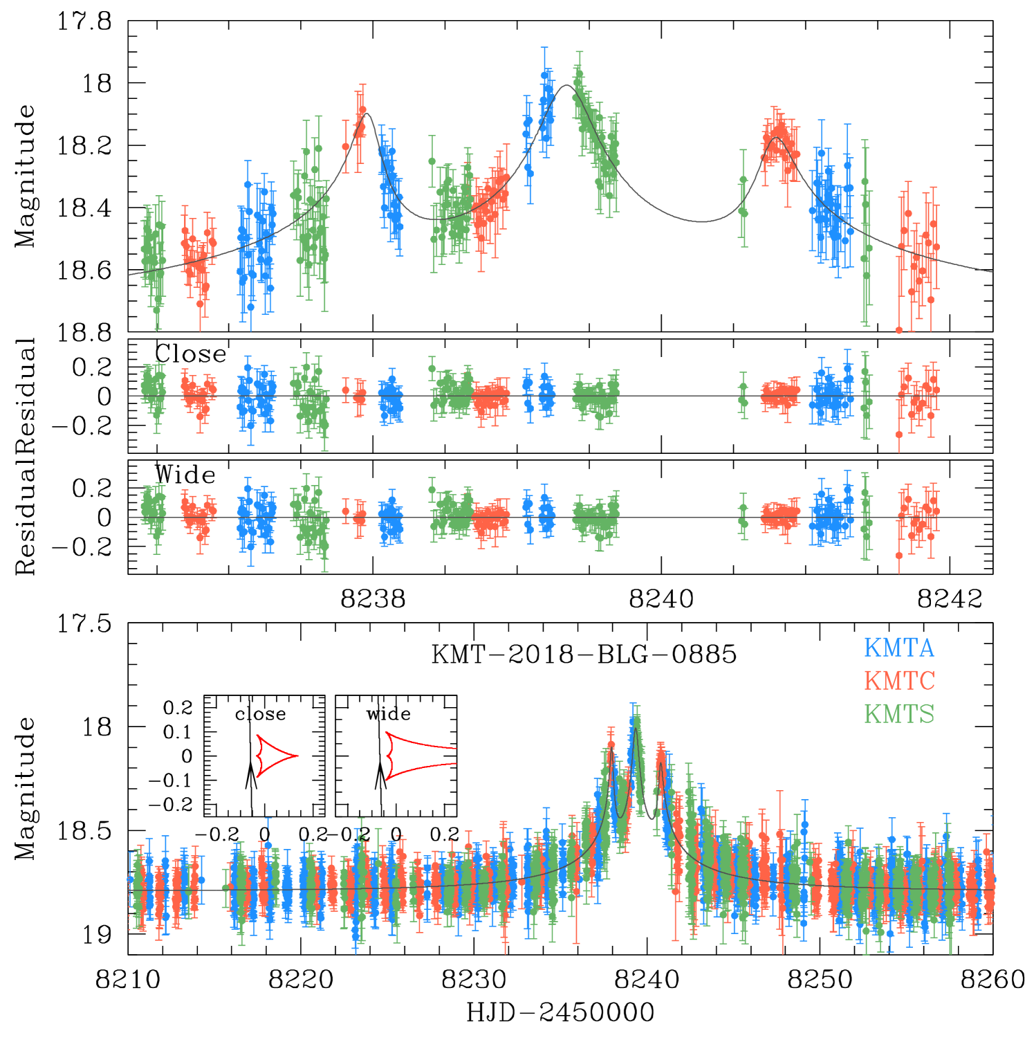
The light curve of the event is shown in Figure 2. It is characterized by three consecutive bumps appearing around the peak with roughly 2-day gaps between each consecutive pair of bumps. The deviation pattern of these bumps are smooth, suggesting that they were produced by successive approaches of the source close to three cusps of a caustic. For this event, the low mass ratio between the lens components was expected to some extent, because triple-bump anomalies can be produced when a caustic is skewed and its cusps lie on one side of the caustic, for example, the second microlensing planet, OGLE-2005-BLG-071Lb (Udalski et al., 2005).
From detailed modeling of the light curve, we identified two solutions, in which one is in the close binary regime and the other is in the wide binary regime. The binary parameters are for the close solution and for the wide solution. The fact that the binary separations of the close and wide solutions approximately follow the relation indicates that the degeneracy between the solutions is caused by the close–wide degeneracy (Griest & Safizadeh, 1998; Dominik, 1999; An, 2005). We present the full lensing parameters of both solutions in Table 2. As expected from the anomaly pattern, the companion-to-primary mass ratio, , of the lens is small, suggesting that the companion to the lens is likely to be a BD. It was found that the close solution yields a slightly better fit to the data over the wide solution, but the difference between the fits of the two solutions is small with . In Figure 2, we draw the model curve of the close solution, and present the residuals from the close and wide solutions in the region of the anomalies.
| Parameter | Close | Wide |
|---|---|---|
| /dof | ||
| (HJD′) | ||
| (days) | ||
| (rad) | ||
| () |
The two insets in the bottom panel of Figure 2 show the configurations of the close (left inset) and wide (right inset) solutions. Each configuration shows that the three bumps were produced by the source passage close to the three protruding cusps of a caustic generated by a binary lens with a low mass ratio. The normalized source radius could not be tightly constrained and only its upper limit, , can be set.
3.3 KMT-2019-BLG-0297
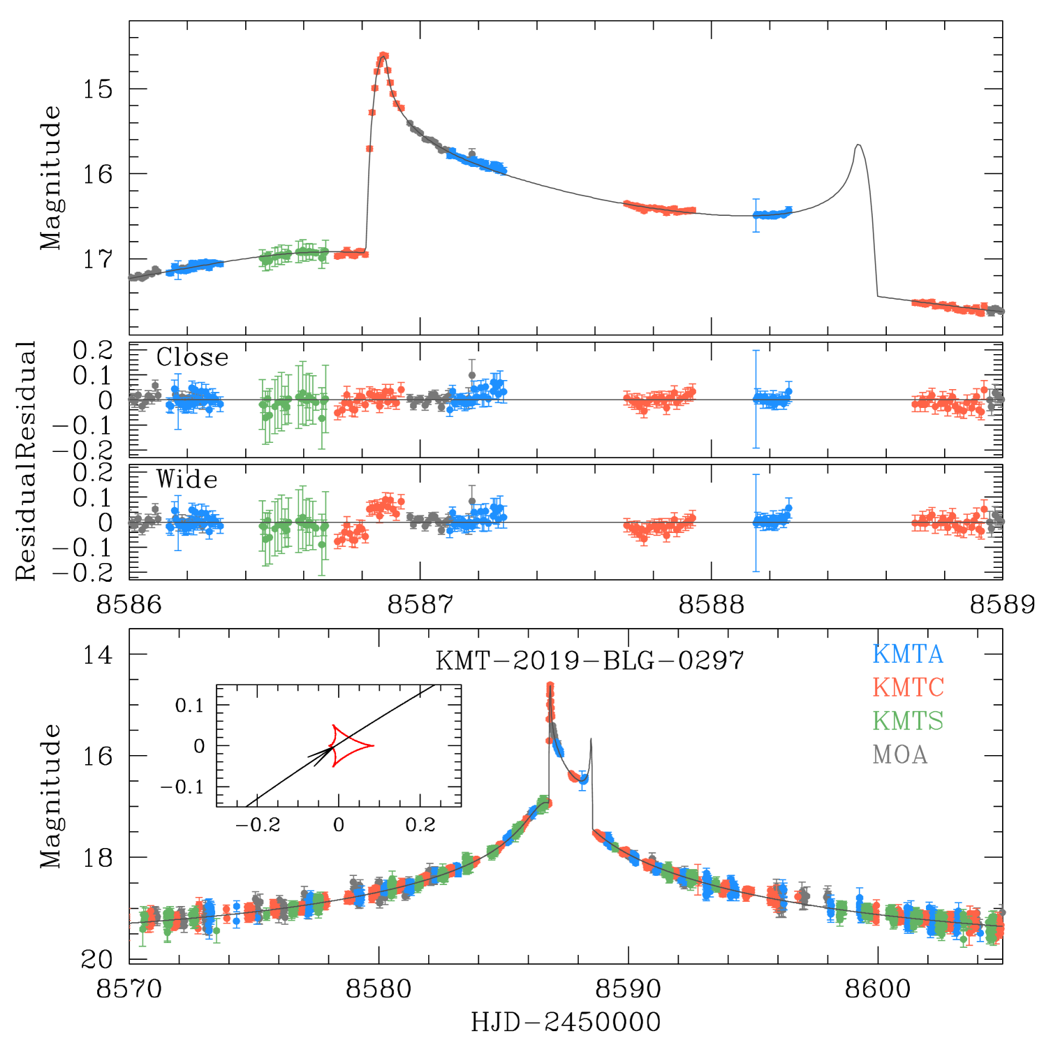
The source coordinates of the event KMT-2019-BLG-0297 are (RA, DEC)18:00:15.19, -28:57:55.01), . The source lies in the two overlapping KMTNet prime fields of BLG03 and BLG43, toward which the event was observed with a 0.25 hr combined cadence. In the 2019 season, the AlertFinder system was operational, and the event was detected in its early stage on April 5 (), when the event was magnified by magnitude from the baseline of . The event was independently detected by the MOA survey three days after the KMTNet alert.
| Parameter | Standard | Higher order | |
|---|---|---|---|
| Close | Wide | (close) | |
| /dof | |||
| (HJD′) | |||
| (days) | |||
| (rad) | |||
| () | |||
| – | – | ||
| – | – | ||
| (yr-1) | – | – | |
| (yr-1) | – | – | |
The lensing light curve of the event constructed with the combination of the KMTNet and MOA data is shown in Figure 3. It is characterized by a central anomaly that lasted for about two days. The main feature of the anomaly is the sharp spike centered at caused by a caustic crossing. Binary caustics form closed curves, and thus caustic crossings occur in pairs, that is, when the source enters and exits the caustic. Then, there should be an additional caustic spike, although the data did not cover it. From the curvature of the U-shape pattern after the first caustic spike, it is expected that the second caustic spike occurred at around .
From the detailed modeling of the light curve, it was found that the anomaly in the light curve of the event KMT-2019-BLG-0297 was generated by a close binary () with a low mass ratio between the lens components. The full lensing parameters of the solution are presented in Table 3. We find a weak local minimum of a wide binary lens with , but its fit is worse than that of the close solution by .
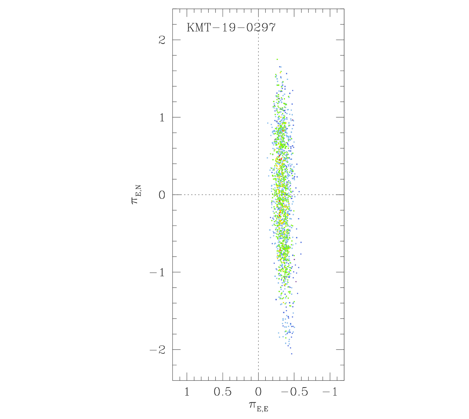
With relatively high-precision data in the wings of the light curve, we test whether the fit further improves with the consideration of higher-order effects. For this check, we conduct an additional modeling considering both the microlens-parallax and lens-orbital effects. It was found that the model considering higher-order effects substantially improved the fit by . The lensing parameters of the higher-order solution are listed in Table 3, and the model curve and residual around the anomaly region are shown in Figure 3. Although turned down, we present the residual of the wide solution for the comparison with the close solution. We note that the variations of the basic lensing parameters with the inclusion of higher-order effects are minor. In Figure 4, we present the scatter plot of points in the MCMC chain on the plane. The plot shows that the east component of the microlens-parallax vector is relatively well constrained, although the north component is not securely measured. As will be discussed in Sect. 5, the measurement of the microlens parallax is important because provides an extra constraint on the physical parameters of the lens. For KMT-2019-BLG-0297, the angular Einstein radius, which is another observable related to the physical lens parameters, can also be constrained because the caustic entrance was densely resolved by the KMTC data, and this yields the normalized source radius , from which the angular Einstein radius is determined as
| (1) |
More details about the determination are discussed in Sect. 4.
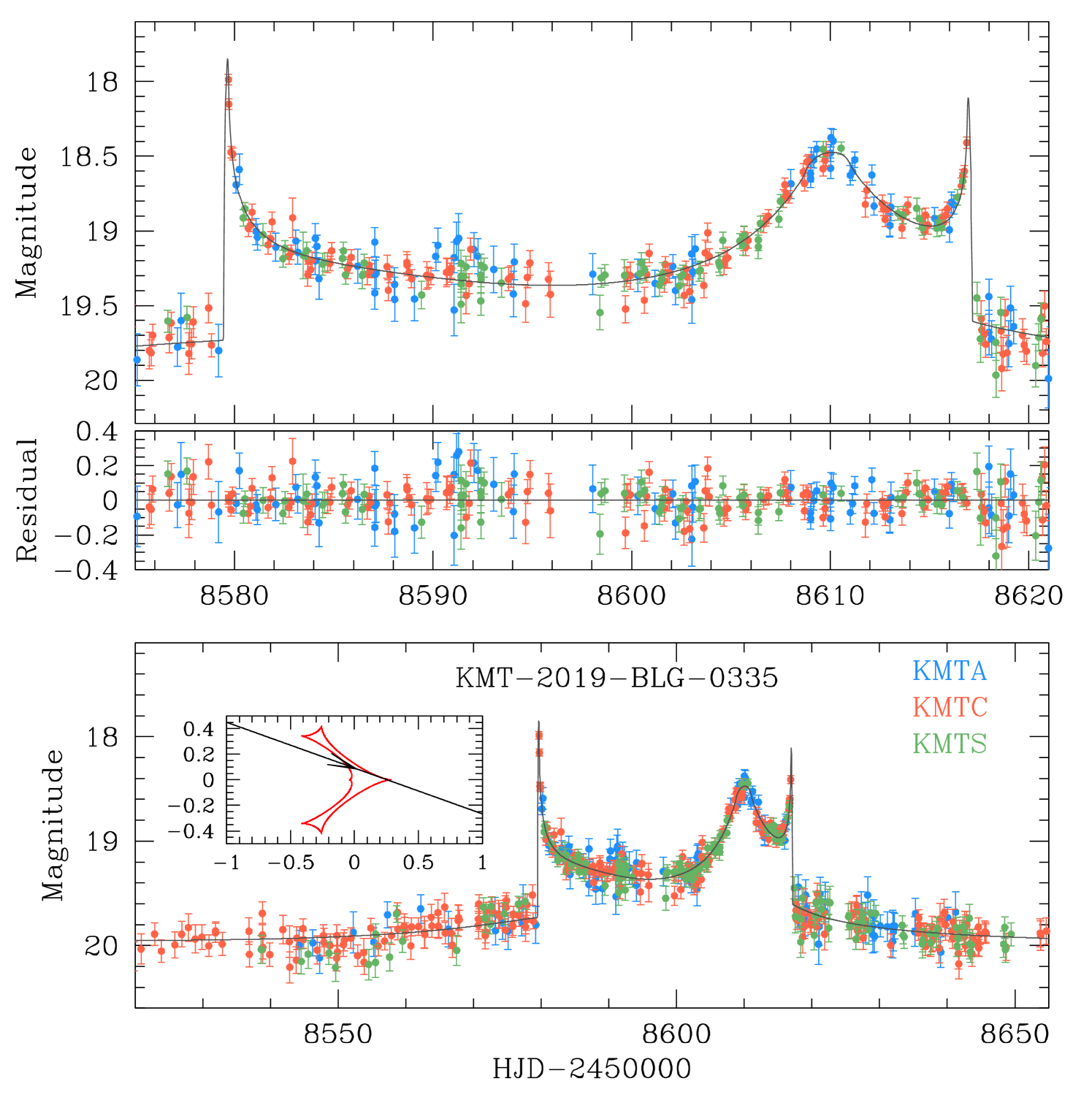
3.4 KMT-2019-BLG-0335
The source of the lensing event KMT-2019-BLG-0335 lies at (RA, DEC)17:31:21.63, -29:35:26.48), . The source position corresponds to the KMTNet BLG11 field, toward which observations were conducted with a 2.5 hr cadence. The lensing magnification of the source flux began before the start of the 2019 observation season, and the event was detected on 2019 April 9 () after the event went through a substantial magnification by the caustic crossing of the source.
| Parameter | Value |
|---|---|
| /dof | |
| (HJD′) | |
| (days) | |
| (rad) | |
| () |
Figure 5 shows the lensing light curve of KMT-2019-BLG-0335. It is characterized by three distinctive anomaly features: the two spikes at and 8616.3 and the bump centered at appearing between the caustic spikes. From the characteristic pattern, the spike features are likely to result from caustic crossings. From the location of the bump appearing in the U-shape region between the caustic-crossing features, it is expected that the bump was produced by the asymptotic approach of the source close to a fold of a caustic as the source proceeded inside the caustic. Although the rising part of the first spike feature and the falling part of the second spike feature were not covered by the data, the pattern of the caustic-crossing features can be well delineated by the data just after the first spike and before the second spike.
Detailed modeling of the light curve yields a unique solution with binary parameters of , indicating that the anomaly features were produced by a close binary with a low-mass companion. We list the full lensing parameters in Table 4, and the model curve and residual around the anomaly region are presented in Figure 5. The time scale of the event, days, is fairly long, but it is difficult to constrain the higher-order lensing parameters due to the substantial photometric errors of the data caused by the faintness of the source. The normalized source radius is measured, although its uncertainty is fairly big due to the incomplete coverage of the caustic crossings.
The inset in the bottom panel of Figure 5 shows the configuration of the lens system. The caustic is similar to that of KMT-2018-BLG-0321 with the two peripheral caustics connected with the central caustic by narrow bridges, indicating that the binary is at the boundary between the close and intermediate regimes. The source entered the upper left side of the central caustic, passed along the upper right fold of the caustic, and exited the lower right side of the caustic. The caustic entrance and exit produced the spike features, and the bump was generated by the source approach to the caustic fold.
| Events | (as) | ||||
|---|---|---|---|---|---|
| KMT-2018-BLG-0321 | 16.500 | ||||
| KMT-2018-BLG-0885 | 14.384 | ||||
| KMT-2019-BLG-0297 | 14.382 | ||||
| KMT-2019-BLG-0335 | 14.396 |
4 Source stars and Einstein radii
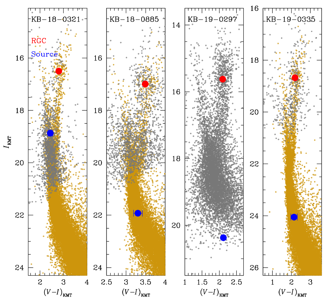
In this section, we specify the source stars of the individual lensing events and estimate angular Einstein radii for the events with measured normalized source radii. For each event, the source is specified by measuring its reddening and extinction-corrected (de-reddened) color and magnitude. The measured source color and magnitude are used to deduce the angular source radius, from which the angular Einstein radius is estimated from the relation in Equation (1).
Figure 6 shows the source locations of the individual lensing events in the instrumental color-magnitude diagrams (CMDs) of stars lying adjacent to the source stars constructed from pyDIA (Albrow, 2017) photometry of the KMTC images. The - and -band magnitudes of each source were estimated from the regression of the light curve data measured using the same pyDIA photometry with respect to the lensing magnification. For the three events KMT-2018-BLG-0321, KMT-2018-BLG-0885, and KMT-2019-BLG-0335, the -band source magnitudes could not be securely measured due to the poor quality of the -band data, although their -band magnitudes were measured. In these cases, we first combine the two sets of CMDs, one constructed from the pyDIA photometry of stars in the KMTC image and the other for stars in the Baade’s window observed with the use of the Hubble Space Telescope (Holtzman et al., 1998), align the two CMDs using the centroids of the red giant clump (RGC) in the individual CMDs, and then estimate the source color as the median values for stars in the main-sequence branch of the HST CMD with -band magnitude offsets from the RGC centroid corresponding to the measured values. The estimated instrumental colors and magnitudes of the source stars, , and RGC centroids, , for the individual events are listed in Table 5.
| Event | (mas) | (mas yr-1) |
|---|---|---|
| KMT-2018-BLG-0321 | ||
| KMT-2018-BLG-0885 | ||
| KMT-2019-BLG-0297 | ||
| KMT-2019-BLG-0335 |
For the calibration of the source colors and magnitudes, we use the RGC centroid, for which its de-reddened values are well defined (Bensby et al., 2013; Nataf et al., 2013), as a reference (Yoo et al., 2004). By measuring the offsets in color and magnitude, , of the source star from those of the RGC centroid, the de-reddened values are estimated as . The estimated de-reddened source colors and magnitudes of the individual events are listed in Table 5. According to the estimated de-reddened colors and magnitudes, it is found that the source of KMT-2018-BLG-0321 is a G-type turnoff star, and those of the other events are main-sequence stars with spectral types ranging from late G to early K.
The angular radii of the source stars were deduced from their measured colors and magnitudes. For this, we first converted color into color using the Bessell & Brett (1988) relation, and then estimated the angular source radius using the Kervella et al. (2004) relation between and . For the events with measured normalized source radii, the angular Einstein radii were estimated using the relation in Equation (1). The estimated angular radii of the source stars and Einstein rings of the individual events are listed in Table 6. Also listed are the relative proper motions between the lens and source estimated by . In the cases of the events KMT-2018-BLG-0321 and KMT-2018-BLG-0885, for which only the upper limits of are constrained, we list the lower limits of and .
| Events | () | () | (kpc) | (AU) |
|---|---|---|---|---|
| KMT-2018-BLG-0321 | ||||
| KMT-2018-BLG-0885 (close) | ||||
| (wide) | – | – | ||
| KMT-2019-BLG-0297 | ||||
| KMT-2019-BLG-0335 |
5 Physical lens properties
The basic lensing observable constraining the physical parameters of the lens mass and distance to the lens is the Einstein time scale , which is related to the physical parameters by
| (2) |
where . Besides this observable, the lens mass and distance can be additionally constrained by measuring the extra observables of and . If both of these extra observables are simultaneously measured, the physical lens parameters can be uniquely determined by the relation
| (3) |
where is the parallax of the source, and denotes the distance to the source (Gould, 2000). For KMT-2019-BLG-0297, both of these extra parameters are measured, but the uncertainty of the measured microlens parallax is large. For the event KMT-2019-BLG-0335, the Einstein radius is measured, but the values of are not constrained. For the KMT-2018-BLG-0321 and KMT-2018-BLG-0885, none of the extra observables are measured, and only the lower limits of are constrained. Due to the incompleteness of the observables, we estimated the physical lens parameters by conducting Bayesian analyses based on the available observables of the individual events.
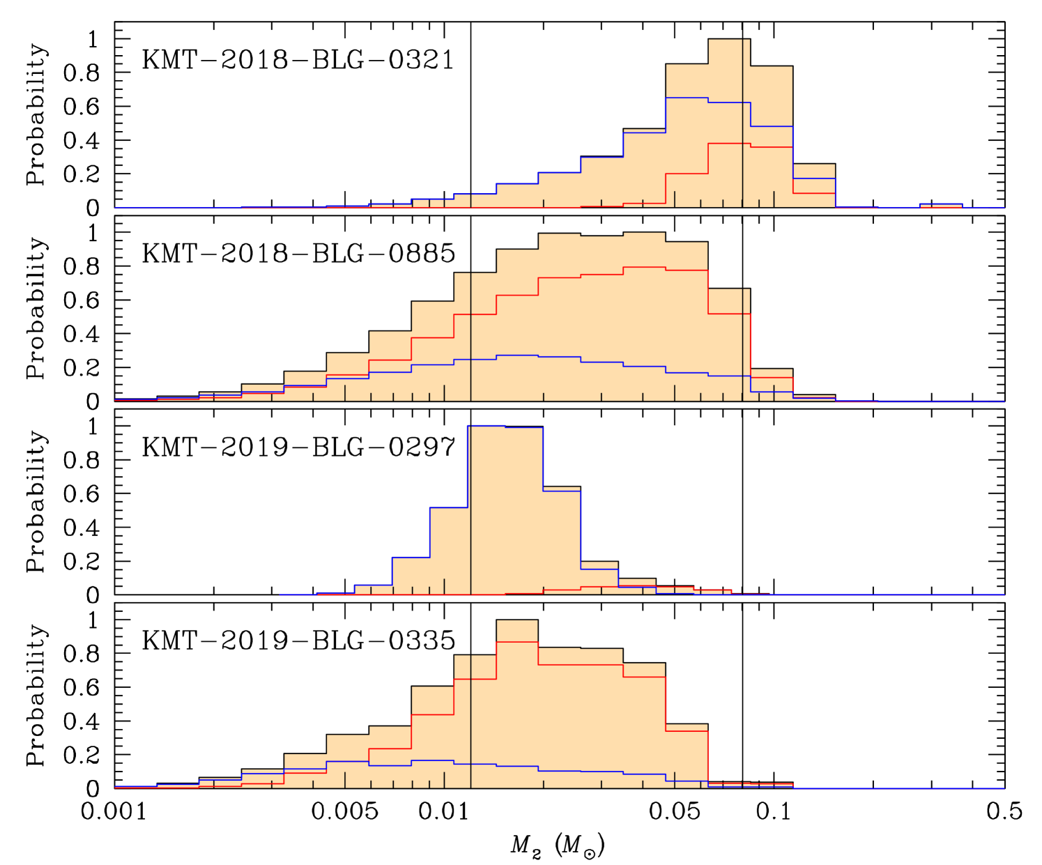
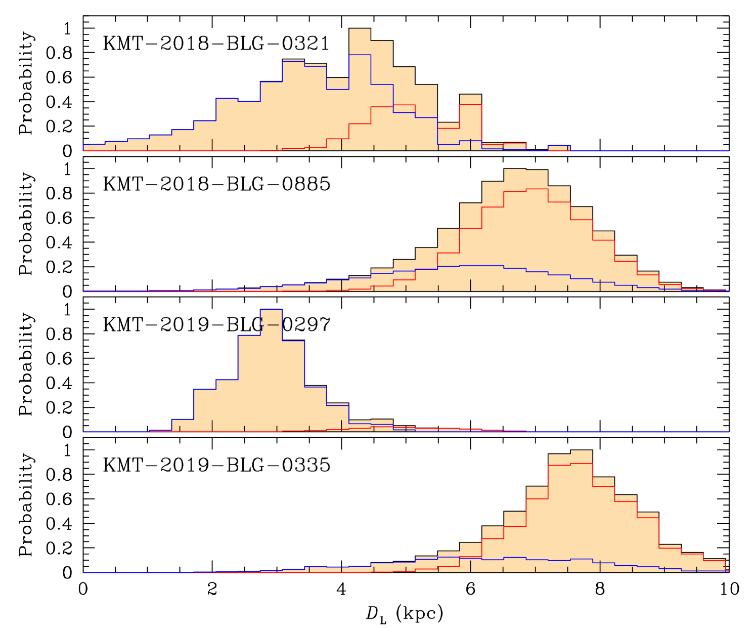
The Bayesian analysis for each event was carried out by first generating a large number () of artificial microlensing events from a Monte Carlo simulation with the use of a prior Galactic model. The Galactic model defines the positions, velocities, and masses of astronomical objects in the Galaxy, and we adopted the Jung et al. (2021) model. For each simulated event, we computed the lens observables of the Einstein time scale, , Einstein radius, , and microlens parallax, . Here, denotes the transverse lens-source speed. We then constructed a Bayesian posterior distributions of the lens mass and distance by imposing a weight to each simulated event of , where and denote the measured value of the observable and its uncertainty, respectively. In the case of the event for which only the lower limit of is constrained, we set for events with .
The posterior distributions for the mass of the lens companion and distance to the lens system are presented Figures 7 and 8, respectively. In each distribution, we mark three curves, in which the blue and red curves represent the contributions by the disk and bulge lens populations, respectively, and the black curve is sum of the two contributions. The two vertical lines in the mass posteriors represent the boundaries between planetary, BD, and stellar lens populations. We set the boundary between planets and BDs as () and that between BDs and stars as .
| Events | |||||
|---|---|---|---|---|---|
| KMT-2018-BLG-0321 | 59 | 3 | 38 | 75 | 25 |
| KMT-2018-BLG-0885 | 68 | 25 | 7 | 29 | 71 |
| KMT-2019-BLG-0297 | 66 | 34 | 0 | 94 | 6 |
| KMT-2019-BLG-0335 | 66 | 33 | 10 | 22 | 78 |
In Table 7, we summarize the estimated physical lens parameters, including , , , and , where denotes the projected separation between the binary lens components. We take the median values of the posterior distributions as representative values, and the uncertainties are estimated as the 16% and 84% of the distributions. In Table 8, we list the probabilities for the lens companion to be in the planetary (), BD (), and stellar () mass regimes. In all cases of the events, the median values of lie in the BD mass regime, and the probabilities for the lens companion to be in the BD mass regime are high. For the events KMT-2018-BLG-0885, KMT-2019-BLG-0297, and KMT-2019-BLG-0335, the probabilities for the lens companions to be in the planetary mass regime are , 34%, and 33%, respectively, and thus it is difficult to completely rule out the possibility that the companions are giant planets. Also listed in Table 8 are the probabilities for the lens to be in the disk, , and in the bulge, . It turns out that KMT-2019-BLG-0297L is very likely to be in the disk mainly from the 2-dimensional gaussian constraint of the measured microlens-parallax, that is, Figure 4.
6 Summary and conclusion
We investigated the microlensing data acquired during the 2018, 2019, and 2020 seasons by the KMTNet survey in order to find lensing events produced by binaries with brown-dwarf companions. For this investigation, we conducted systematic analyses of anomalous lensing events observed during the seasons, and picked out candidate BD binary-lens events by applying the selection criterion that the companion-to-primary mass ratio was less than 0.1. From this procedure, we identified four candidate events with BD companions, including KMT-2018-BLG-0321, KMT-2018-BLG-0885, KMT-2019-BLG-0297, and KMT-2019-BLG-0335. No candidates were identified in the 2020 season, which was severely affected by the Covid-19 pandemic.
We estimated the masses of the lens companions by conducting Bayesian analyses using the measured observables of the individual events. From this estimation, it was found that the probabilities for the masses of the companions to be in the BD mass regime were high with 59%, 68%, 66%, and 66% for KMT-2018-BLG-0321, KMT-2018-BLG-0885, KMT-2019-BLG-0297, and KMT-2019-BLG-0335, respectively. We plan to report additional BD binary-lens events from the investigation of the data acquired in the 2021 and 2022 seasons. Together with the previous 6 BD events (OGLE-2016-BLG-0890, MOA-2017-BLG-477, OGLE-2017-BLG-0614, KMT-2018-BLG-0357, OGLE-2018-BLG-1489, and OGLE-2018-BLG-0360) reported in paper I plus KMT-2020-BLG-0414LB recently reported by Zang et al. (2021), the KMTNet sample will be useful for a future statistical analysis on the properties of BDs.
Acknowledgements.
Work by C.H. was supported by the grants of National Research Foundation of Korea (2019R1A2C2085965). This research has made use of the KMTNet system operated by the Korea Astronomy and Space Science Institute (KASI) at three host sites of CTIO in Chile, SAAO in South Africa, and SSO in Australia. Data transfer from the host site to KASI was supported by the Korea Research Environment Open NETwork (KREONET). The MOA project is supported by JSPS KAKENHI Grant Number JSPS24253004, JSPS26247023, JSPS23340064, JSPS15H00781, JP16H06287, and JP17H02871. J.C.Y. acknowledges support from NSF Grant No. AST-2108414. Y.S. acknowledges support from NSF Grant No. 2020740. W.Z. and H.Y. acknowledge support by the National Science Foundation of China (Grant No. 12133005). C.R. was supported by the Research fellowship of the Alexander von Humboldt Foundation.References
- Albrow et al. (2009) Albrow, M., Horne, K., Bramich, D. M., et al. 2009, MNRAS, 397, 2099
- Albrow (2017) Albrow, M. 2017, MichaelDAlbrow/pyDIA: Initial Release on Github,Versionv1.0.0, Zenodo, doi:10.5281/zenodo.268049
- An (2005) An, J. H. 2005, MNRAS, 356, 1409
- Batista et al. (2011) Batista, V., Gould, A., Dieters, S. et al. 2011, A&A, 529, 102
- Bensby et al. (2013) Bensby, T. Yee, J.C., Feltzing, S. et al. 2013, A&A, 549, A147
- Bessell & Brett (1988) Bessell, M. S., & Brett, J. M. 1988, PASP, 100, 1134
- Bond et al. (2001) Bond, I. A., Abe, F., Dodd, R. J., et al. 2001, MNRAS, 327, 868
- Cassan (2008) Cassan, A. 2008, A&A, 491, 587
- Dominik (1999) Dominik, M. 1999, A&A, 349, 108
- Schneider & Weiss (1986) Schneider, P., & Weiss, A. 1986, A&A, 164, 237
- Gould (1992) Gould, A. 1992, ApJ, 392, 442
- Gould (2000) Gould, A. 2000, ApJ, 542, 785
- Gould & Loeb (1992) Gould, A. & Loeb, A. 1992, ApJ, 396, 104
- Gould (2022) Gould, A. 2022, arXiv:2209.12501
- Gould et al. (2022) Gould, A., Han, C., Weicheng, Z., et al. 2022, A&A, 664, A13
- Grether & Lineweaver (2006) Grether, D, & Lineweaver, C. H. 2006, ApJ, 640, 1051
- Griest & Safizadeh (1998) Griest, K., & Safizadeh, N. 1998, ApJ, 500, 37
- Han & Gould (2003) Han, C., & Gould, A. 2003, ApJ, 592, 172
- Han et al. (2020) Han, C., Lee, C.-U., Udalski, A., et al. 2020, AJ, 159, 134
- Han et al. (2022) Han, C., Ryu, Y.-H., Shin, I.-G., et al. 2022, A&A, 667, A64
- Holtzman et al. (1998) Holtzman, J. A., Watson, A. M., Baum, W. A., et al. 1998, AJ, 115, 1946
- Jung et al. (2021) Jung, Y. K., Han, C., Udalski, A., et al. 2021, AJ, 161, 293
- Jung et al. (2022) Jung, Y. K., Zang, W., Han, C., et al. 2022, AJ, 164, 262
- Kervella et al. (2004) Kervella, P., Thévenin, F., Di Folco, E., & Ségransan, D. 2004, A&A, 426, 29
- Kim et al. (2018a) Kim, D.-J., Kim, H.-W., Hwang, K.-H., et al., 2018a, AJ, 155, 76
- Kim et al. (2018b) Kim, H.-W., Hwang, K.-H., Shvartzvald, Y., et al. 2018b, arXiv:1806.07545
- Kim et al. (2016) Kim, S.-L., Lee, C.-U., Park, B.-G., et al. 2016, JKAS, 49, 37
- Nataf et al. (2013) Nataf, D. M., Gould, A., Fouqué, P. et al. 2013, ApJ, 769, 88
- Shvartzvald et al. (2016) Shvartzvald, Y., Maoz, D., Udalski, A., et al. 2016, MNRAS, 457, 4089
- Shvartzvald et al. (2019) Shvartzvald, Y., Yee, J. C., Skowron, J., et al. 2019, AJ, 157, 106
- Skowron et al. (2011) Skowron, J., Udalski, A., Gould, A., et al. 2011, ApJ, 738, 87
- Tsapras et al. (2019) Tsapras, Y., Street, R. A., Hundertmark, M., et al. 2019, PASP, 131, 124401
- Udalski et al. (2005) Udalski, A., Jaroszyński, M., Paczyński, B, et al. 2005, ApJ, 628, L109.
- Udalski et al. (2015) Udalski, A., Szymański, M. K., & Szymański, G. 2015, Acta Astron., 65, 1
- Whitworth al. (2007) Whitworth, A., Bate, M. R., Nordlund, A. A., Reipurth, B., & Zinnecker, H. 2007, in Protostars and Planets, Vol. 951 ed. V. B. Reipurth, D. Jewitt, & K. Keil (Tucson: Univ. Arizona Press), 459
- Yee et al. (2012) Yee, J. C., Shvartzvald, Y., Gal-Yam, A., et al. 2012, ApJ, 755, 102
- Yoo et al. (2004) Yoo, J., DePoy, D.L., Gal-Yam, A. et al. 2004, ApJ, 603, 139
- Zang et al. (2021) Zang, W., Han, C., Kondo, I., et al. 2021, Research in Astronomy and Astrophysics, 21, 239