Probing Chiral Kitaev Spin Liquids via Dangling Boundary Fermions
Abstract
Identifying experimental probes capable of diagnosing extreme quantum behavior is widely regarded as one of the foremost challenges in modern condensed matter physics. Here, we propose a novel approach for detecting chiral Kitaev spin liquid states through measurements of the local dynamical spin structure factor on the boundary using scanning tunneling microscopy (STM). We specifically focus on unpaired (“dangling”) Majorana fermions, which naturally emerge along boundaries of Kitaev spin liquids, and can serve as indicators of chiral boundary modes under broad conditions, thereby offering a clear signature of these exotic quantum states.
I Introduction
The exact solution of the famous honeycomb Kitaev model [1] has sparked significant efforts to discover materials that host chiral Kitaev spin liquids (KSLs). These spin liquids are characterized by topologically robust chiral edge modes propagating along the boundary, and may support non-Abelian bulk excitations binding Majorana zero modes. Notably, it has been shown that the bond-directional spin interactions of the Kitaev model naturally arise between effective spin-1/2 magnetic moments in spin-orbit-coupled and materials [2]. In turn, this insight has driven the discovery of several candidate materials where the microscopic spin Hamiltonian is believed to closely approximate the Kitaev model [3, 4, 5, 6].
These “Kitaev materials” include the honeycomb iridates, such as Na2IrO3 [7, 8, 9, 10, 11, 12], -Li2IrO3 [13, 14] , H3LiIr2O6 [15], and Ag3LiIr2O6 [16], as well as -RuCl3 [17, 18, 19, 20, 21, 22, 23, 24, 25]. Although several material candidates have been identified, diagnosing spin-liquid states through conventional experimental probes, such as inelastic neutron scattering or thermodynamic measurements, remains extremely challenging. Attempts to detect a chiral KSL state in -RuCl3 via the predicted quantization of the thermal Hall effect have also been inconclusive, mainly due to sample dependence and the difficulty of disentangling magnetic and phonon contributions to the thermal Hall conductivity [26, 27, 28, 29, 30, 31, 32, 33, 34]. Hence, a natural question to ask is whether alternative experimental probes could provide more definitive evidence of this novel state of matter.
Inelastic electron tunneling spectroscopy [35, 36] has been recently identified as an effective probe of magnetic excitations in two-dimensional insulators [37, 38, 39]. It has also been successfully applied to resolve spin waves in interacting magnetic atoms [40, 41], and could even offer insights into localized boundary modes [42, 43, 44]. This spectroscopic technique uses the magnetic insulator as a tunneling barrier between two metallic electrodes, and measures inelastic tunneling processes where an electron tunneling through the magnetic insulator creates spin excitations. In the context of Kitaev materials, a recent experimental work employed this technique to probe the magnetic excitations of atomically thin -RuCl3 [45]. At the same time, several theoretical studies have proposed a local version of this technique, corresponding to inelastic scanning tunneling microscopy (STM), for observing key hallmarks of chiral KSLs, including the chiral Majorana edge modes [46] and the Majorana zero modes [47, 48, 49, 50, 51].
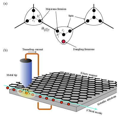
In particular, Feldmeier et al. [46] proposed to use such an inelastic STM setup [see Fig. 1(b)] in order to probe the local spin dynamics in a chiral KSL and detect gapless spin excitations along its boundary. From the inelastic STM measurement, the local dynamical spin structure factor (DSSF) can be extracted as the derivative of the tunneling conductance with respect to the bias voltage . More precisely,
| (1) |
where is the real-space DSSF, and is the electron tunneling amplitude between the substrate and the STM tip at position through site of the spin system in between [see Fig. 1(b)]. Since this tunneling amplitude decays exponentially on the nanometer scale, this approach allows the detection of the local DSSF with a spatial resolution close to the atomic size.
As explained in Ref. [46], inelastic STM can be employed to measure the gapless spin excitations near the boundary, which are in stark contrast to the gapped spin excitations in the bulk of the system. Since the corresponding gapless edge mode is necessarily of fermionic character, it is directly indicative of spin fractionalization and thus reveals an underlying spin liquid. At the same time, this kind of inelastic STM measurement along a clean boundary is insufficient to diagnose the chiral nature of the spin liquid because it cannot distinguish between chiral and helical gapless edge modes.
Here, we propose a definitive STM signature of chiral KSLs that is revealed by ubiquitous edge disorder but ultimately originates from “dangling” Majorana fermions of the underlying Kitaev model. These dangling edge fermions are directly coupled to the chiral edge fermions by the external magnetic field that produces the chiral KSL by gapping out the bulk fermion spectrum [49, 50, 51, 52]. Hence, this significant (but generally overlooked) effect modifies the spin dynamics along the edge to linear order in the field and gives rise to a range of observable consequences. In the companion paper [53], we establish that a zigzag edge of the KSL supports a pronounced low-energy peak in the local DSSF whose energy scales linearly with only one component of the field. In this paper, we demonstrate that edge disorder generically produces additional resonance peaks in the local DSSF that exhibit the same linear energy scaling but can also be leveraged to diagnose the chiral nature of the KSL. In particular, the hybridization of the dangling fermions and the chiral edge mode creates a topological obstruction to Anderson localization [54, 55, 56], which is not present in non-chiral KSLs supporting helical edge modes. Consequently, the peak width scales linearly with the field in chiral KSLs, while it is largely field independent for non-chiral KSLs. From a more general perspective, the dangling fermions act as “witnesses” to the topologically protected chiral edge mode, providing a unique perspective on the chiral nature of the bulk spin liquid.
II Model
To study the boundary modes of the KSL under an external field, we consider the following Hamiltonian:
| (2) |
where
| (3) |
is the exactly solvable Kitaev model [1],
| (4) | |||||
refers to generic non-Kitaev symmetric spin-exchange interactions, and
| (5) |
represents a Zeeman coupling to an external magnetic field . Here denotes nearest neighbor bonds with three different orientations labeled by , while () are the components of the external magnetic field and () are antiferromagnetic Kitaev spin exchange interactions. This model is exactly solvable in absence of magnetic field () and non-Kitaev interactions (), giving rise to a quantum spin liquid ground state with two types of elementary excitations. One type corresponds to gapped or gapless matter fermions, depending the anisotropy of the Kitaev interactions, while the other one corresponds to emergent fluxes. A single flux excitation is also known as “vison” and has a finite energy gap . The KSL phase is stable for a finite range of magnetic fields and non-Kitaev interactions [57], although a magnetic field immediately gaps out any gapless matter fermions.
As illustrated in Fig. 1, the KSL is obtained by expressing the spin operator as a bilinear product of Majorana fermion operators [1], , where , and labels the lattice site. In general, the fermions correspond to matter-field excitations, while the fermions describe gauge fields coupled to them. For an infinite lattice, the fermions pair up and form the gauge fields , which are conserved quantities and take uniform values (assuming and , with being the two sublattices of the honeycomb lattice) in the standard gauge choice for the zero-flux sector. For a finite lattice, however, the Z2 gauge fields are no longer well defined for the missing bonds on the boundary. These unpaired fermions associated with missing bonds, as indicated by red dots in Fig. 1, are referred to as “dangling fermions” [49, 50, 51, 52]. The dangling fermions correspond to zero-energy boundary modes of the pure Kitaev model and must be included in the low-energy description of the spin dynamics on the boundary.
II.1 Effective Hamiltonian under field
In this work, we are only interested in low-energy dynamics below , which corresponds to the zero-flux sector of the Kitaev model. In this regime, the spin dynamics is completely determined by the spin excitations generated by the “dangling spins” on the boundary that create “dangling fermions”. For that purpose, we first introduce a relevant effective Hamiltonian governing the low-energy dynamics.
Projecting into the zero-flux sector yields two distinct contributions. The first one originates from the Kitaev Hamiltonian and has a quadratic form in terms of the fermions:
| (6) |
where the sum runs over all non-equivalent nearest neighbor bonds, and refer to the two sublattices of the honeycomb lattice, and we are adopting the standard gauge choice for the zero-flux sector [1]. The second contribution arises from the Zeeman coupling to an external field, . Projected into the zero-flux sector, this term generates a boundary contribution,
| (7) |
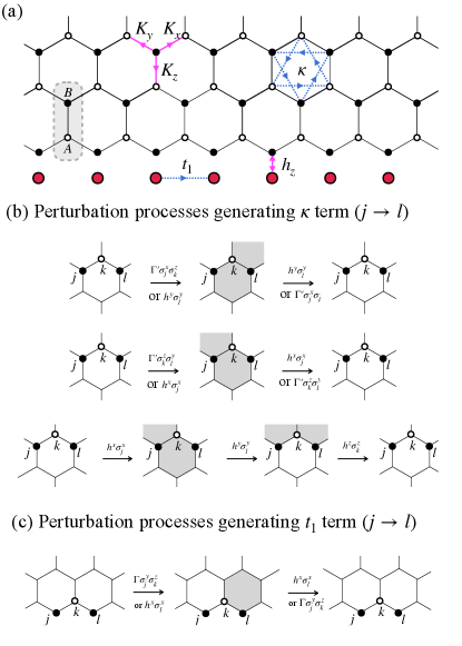
which is linear in the magnetic field and hybridizes each dangling fermion (where is , , or , depending on ) with the matter fermion via the -th component of the Zeeman field. The two terms described in this paragraph are illustrated by the pink solid arrows in Fig. 2(a).
Higher-order processes generate further symmetry-allowed terms, as indicated by blue dashed arrows in Fig. 2(a). Given the dominance of the Kitaev interactions, we restrict our attention to terms arising from leading-order perturbations. Additionally, we assume that these interactions do not alter the quasiparticle picture, retaining only quadratic terms in the effective Hamiltonian. In the bulk, higher-order processes generate the effective three-spin interaction that immediately gaps out any gapless bulk fermions [1]:
| (8) |
where is a permutation of in each term, and denotes a three-site path formed by two consecutive nearest-neighbor bonds and . This effective interaction preserves the integrability of the model. The scaling of with respect to is given by [58], where originates from a second-order process involving the term the and Zeeman coupling term, while arises from a third-order contribution in [1]. The factor of in accounts for two different processes, illustrated by the first two lines of Fig. 2(b), which contribute to the same matrix element. On the boundary, higher-order processes endow the dangling fermions with a finite hopping term:
| (9) |
This hopping arises, for example, from second-order perturbation processes involving the term and the Zeeman coupling term, as shown in Fig. 2(c), which give a hopping amplitude . In the following, we consider only the nearest-neighbor hopping term, denoted as . Hopping terms beyond nearest neighbors merely affect the dispersion of the boundary mode without introducing any qualitatively new effects.
To summarize, the low-energy physics is described by the effective Hamiltonian
| (10) |
which takes a quadratic form,
| (11) |
in the fermionic representation. Here , and refers to the components of the Majorana-fermion vector,
| (12) |
with being the number of lattice sites, the number of dangling fermions on the boundary, and the spin component corresponding to a given dangling fermion (see, e.g., Fig. 2).
The effective Hamiltonian can be diagonalized through a unitary transformation,
| (13) |
where , and is an unitary matrix. The -th column of this matrix, , satisfies the eigenvalue equation
| (14) |
where is the matrix of the quadratic Hamiltonian in Eq. (11). The eigenvalues appear in pairs due to particle-hole symmetry. After applying the transformation in Eq. (13), the effective Hamiltonian takes a diagonal form
| (15) |
To distinguish the and fermions, we introduce the notations and . Moreover, we define , where is a vector and a vector. The transformation in Eq. (13) leads to two equations
| (16) |
where and are the -th components of and , respectively. The inverse transformation is given by
| (17) |
II.2 Local spin structure factor
Our primary focus is the local dynamic spin structure factor (DSSF) on boundary lattice sites ,
| (18) |
which can be measured by STM. We specifically consider the spin components corresponding to the dangling fermions at the boundary sites , as they excite low-energy boundary fermion modes without generating gauge fluxes with a finite energy gap .
In the Majorana fermion representation, the local DSSF reduces to a convolution of two Majorana fermion spectral functions :
| (19) | |||||
where we have abbreviated the flavor index of the dangling fermions for notation convenience, and
| (20) |
Since , the spectral function satisfies the sum rule
| (21) |
while the off-diagonal elements satisfy
| (22) |
due to the anti-commutation relation of the Majorana fermions: . Furthermore, since , the DSSF satisfies the sum rule
| (23) |
The Majorana fermion spectral functions can be computed by expressing the operators in terms of the quasi-particle operators that diagonalize :
| (24) | |||||
where
| (25) |
and represents an excited single-quasiparticle state.
III STM response for a uniform boundary
A distinctive feature of the chiral KSL, setting it apart from the non-chiral KSL as well as conventional ordered magnets, is the existence of a gapless chiral boundary mode. Detecting this chiral boundary mode is essential for experimentally identifying this exotic state of matter. In the companion paper [53], we studied the local DSSF of the KSL, a quantity accessible by STM, and its field dependence. Specifically, we demonstrated that the hybridization between the dangling fermions and the gapless boundary mode leads to a pronounced peak in the local DSSF whose energy scales linearly with only one component of the magnetic field.
The goal of this work is to explore how STM can be used to distinguish the chiral KSL from the non-chiral one, which lacks chiral boundary modes, and more broadly, from other magnetic states with low-energy boundary modes. To achieve this goal, we proceed in two steps. In this section, we consider a clean and uniform boundary by adopting periodic boundary conditions (PBC) along the boundary direction (cylindrical lattice) and compare the local DSSFs for the chiral and non-chiral KSL phases. Given that the distinction between the chiral and non-chiral KSLs is inevitably complicated by disorder, we address this important effect in the next section, highlighting how boundary defects can be used to detect universal signatures of the chiral boundary mode.
III.1 Chiral spin liquid phase
We begin by generalizing the analysis in Ref. [53] to arbitrary Kitaev spin exchange. Since we are adopting PBC along the boundary direction, the eigenmodes have a well defined quasi-momentum , where is an integer number that belongs to the interval ( is assumed to be even). For a generic applied magnetic field with , the energy spectrum consists of gapped bulk modes, where a gapless Dirac cone at acquires a finite mass .
In the absence of the hybridization term , the boundary modes consist of two branches: one branch features a flat zero-energy spectrum representing the dangling fermions, while the other branch corresponds to a chiral mode formed by the matter fermions. This chiral mode only exists for and connects the negative-energy Dirac cone at with the positive-energy Dirac cone at .
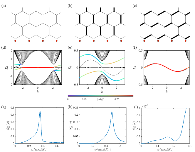
The Zeeman term strongly hybridizes the dangling fermion modes at with the chiral mode, while those at retain their dominant dangling-fermion character because they can only hybridize with bulk matter-fermion modes. Fig. 3(d) shows the boundary modes on one edge before (black dashed line) and after (solid colored line) hybridization for the zigzag boundary depicted in Fig. 3(a).
Fig. 3(a,d,g) show the results obtained from numerical diagonalization of the effective Hamiltonian in Eq. (11). While these calculations are performed for a finite value of the magnetic field, the general structure can be understood by analyzing the small-field limit, , where the spectrum of the boundary modes can be found analytically. For simplicity, we also consider the limit of . An analytical calculation reveals that the crossover momentum is then given by
| (26) |
which recovers in the isotropic limit. The condition holds within the entire non-Abelian phase.
For , the boundary-mode energy is zero to linear order in and has dominant dangling-fermion character, as captured by the wave function
| (27) |
Note that Majorana fermions are real operators, implying that describe the same degree of freedom.
For , the dangling and matter fermions form a hybridized mode with energy linear in . For the zigzag boundary orientation shown in Fig. 3(a), this hybridization is linear in the -component of the external field [53]:
| (28) |
where
| (29) |
is a dimensionless parameter defined by , with being the the localization length of the boundary mode for wave vector . Clearly, the boundary mode only exists for , and the crossover momentum given in Eq. (26) precisely corresponds to .
The minimum of is at where . Around this point, the dispersion reads
The singular square-root behavior of the dispersion leads to the following density of states (DOS) for this hybridized mode,
| (31) |
which is linear in for small energies: . The maximum of is at where . Correspondingly, the DOS has an inverse square-root divergence at the top of the band: .
Next, we investigate the local DSSF, which requires us to compute the matrix elements defined in Eq. (25). For momenta , we have
| (32) |
while for , we obtain
| (33) | |||||
| (34) |
where is a -dependent phase factor. Notably, these matrix elements are explicit functions of the boundary-mode energies . From these results, we obtain the Majorana-fermion spectral functions in Eq. (24):
| (35) | |||||
| (36) | |||||
| (37) |
One can verify that , obeying the sum rule. In contrast, the integrated spectral weight of is less than 1, as some weight is transferred to the bulk modes. The -peak in arises from the quasi-flat modes at , which, in reality, have a finite broadening that is neglected in the small-field analysis above. The factors in , , and originate from the factor in the matrix element given in Eq. (34).
The local DSSF is finally obtained by performing the convolution described in Eq. (19):
| (38) | |||||
where the first term arises from the convolution of the -peak in with , while the second term is connected to two-particle excitations from the hybridized mode at .
Since for small energies, the first term in Eq. (38) dominates over the second one, leading to
| (39) |
Moreover, the first term gives an inverse-square-root singularity at the top of the band, corresponding to
| (40) |
In contrast, the second term results in a regular continuum without any singularities in the entire energy range.
In Fig. 3(g), we show the local DSSF for a finite magnetic field. While the low-energy behavior is rigorously satisfied, the singularity near the band top is smeared out over the interval because the quasi-flat mode, corresponding to the -peak in Eq. (35), has a finite broadening . Nevertheless, the inverse-square-root behavior still approximately applies in a finite energy range below this interval.
III.2 Non-chiral spin liquid phase
Next, we discuss the non-chiral phase of the Kitaev model, where the Kitaev spin exchange is stronger along one of the three bond directions. As shown in Figs. 3(b) and 3(c), there are two possible scenarios depending on the orientation of the strongest bonds relative to the boundary. These two scenarios exhibit distinct boundary excitation spectra, which can be understood by examining the spectrum in the absence of the hybridization term . In the first scenario, where the strongest bonds are perpendicular to the boundary, the boundary spectrum consists of one branch of dangling fermions and another branch of matter fermions [black dotted lines in Fig. 3(e)]. Note that the existence of a matter-fermion boundary mode is linked to boundary sites that are not connected to any dominant bonds as creating a matter-fermion excitation on a dominant bond incurs an energy cost comparable to the largest Kitaev spin exchange. In contrast, for the second scenario, where the strongest bonds are at a angle with respect to the boundary, all lattice sites belong to a dominant bond, and the boundary spectrum thus contains only a single branch of dangling fermions [black dotted line in Fig. 3(f)]. Upon introducing the hybridization term , the two boundary modes in the former case become gapped, whereas the boundary mode in the latter case remains gapless, as indicated by the colored lines in Figs. 3(e) and 3(f).
To make contact with the boundary spectrum of the chiral KSL, we approach the non-chiral phase from the chiral phase by following one of the paths shown in Fig. 4. Along path I, decreases monotonically and vanishes at the phase boundary into the non-chiral phase. Therefore, the dispersive hybridized mode, which exists at in the chiral KSL phase, spans the entire BZ at the phase boundary. In contrast, if we approach the non-chiral phase from path II-1 or II-2, increases to at the phase boundary, and the quasi-flat mode at extends over the whole BZ accordingly.

In the following, we analyze the two scenarios of the non-chiral KSL separately. We start from the scenario in Fig. 3(b) and the corresponding numerical results in Fig. 3(e,h). In this case, the analytical expressions for the small-field limit of the chiral phase remain applicable. However, they reveal different behaviors for both the Majorana-fermion spectral function and the local DSSF. First, the energy spectrum in Eq. (28) becomes gapped due to . In particular, the spectrum is bounded, , by the two finite energies
| (41) | |||
| (42) |
The gapped nature of the spectrum distinguishes the non-chiral phase from the chiral phase where a gapless chiral mode is guaranteed by topology. Due to the quadratic dispersions near the band bottom and the band top , the density of states (DOS) of the boundary modes exhibits inverse-square-root singularities:
| (43) |
The Majorana-fermion spectral function is then confined to the energy interval . Moreover, since the matrix elements in Eq. (25) remain finite in the limits of , the spectral function exhibits the same singular behavior as .
The convolution of the spectral functions in Eq. (19) leads to a two-particle continuum distributed within the energy range . While the convolution produces finite values for and , a logarithmic singularity appears at :
| (44) |
These features obtained to the leading order in explain the local DSSF presented in Fig. 3(h).
Next, we consider the alternative scenario in Fig. 3(c), which corresponds to the numerical results in Fig. 3(f,i). As we discussed above, the dangling fermions can only hybridize with each other as well as the gapped bulk modes, resulting in an effective tight-binding model along the boundary. This effective tight-binding spectrum is gapless, resembling the chiral boundary mode. We also note that the effective hopping amplitude is only finite in the absence of time-reversal symmetry and is not captured by the previous small-field analysis, which only gives rise to a zero-energy mode with the wave function dominated by the dangling fermions [see Eq. (27)].
We calculate the local DSSF numerically for a finite-size lattice. As shown in Fig. 3(i), the DSSF exhibits behavior at small energies, resembling the chiral phase. Additionally, a broad peak appears at the energy corresponding to the top of the boundary band (denoted as ). The spectral intensity is then gradually reduced upon further increasing the energy and vanishes above .
To summarize, the analysis of the chiral and non-chiral KSLs based on the effective low-energy Hamiltonian in Eq. (11) reveals distinct spectral features in the local DSSF. The spectrum remains gapless in the chiral KSL due to the presence of a topologically protected chiral boundary mode. In contrast, for the non-chiral KSL, the spectral response can be either gapped or gapless, contingent on the boundary orientation relative to the dominant bond interaction.
While the characteristic lineshapes observed in both cases can serve as useful indicators, similar low-energy spectral distributions can arise in both chiral and non-chiral KSLs. Moreover, when comparing the local DSSF for the three scenarios in Fig. 3(g,h,i), the distinction between gapped and gapless spectra can become obscured under realistic conditions due to the inevitable presence of disorder. This lack of a clear distinction motivates us to investigate the impact of boundary defects, as their presence may help uncover spectral features unique to the chiral boundary mode, distinguishing it from other types of boundary modes in, e.g., the non-chiral KSL.
IV Effect of disorder along the boundary
Realistic boundaries lack translational invariance due to impurities, vacancies, or corners. As a result of Anderson localization [59], non-chiral boundary modes become localized for any disorder strength. In contrast, the chiral boundary mode remains delocalized because it is protected by the bulk topology. In this section, we explore the measurable effects of this key distinction using STM.
To simulate disorder, we randomly remove lattice sites along the boundary with a finite probability . Although we use as a concrete example, the results presented in this section remain valid for much smaller values of . We leverage the ability of STM to detect the local DSSF directly at or near a single defect (i.e., a vacancy in our simulation). In the chiral KSL, the defect induces a resonant state, observable in the local DSSF as a peak with intrinsic broadening. In contrast, for the non-chiral KSL, the defect generates a truly localized state, which manifests as a sharp peak in the local DSSF, with a width determined entirely by the experimental energy resolution. As we will demonstrate below, the field dependence of the peak width provides a clear distinction between the chiral and the non-chiral KSLs.
IV.1 Chiral Kitaev spin liquid
We first consider the chiral KSL, and start the investigation by examining the Majorana-fermion spectral functions. In the absence of hybridization, the dangling fermions are localized zero-energy modes, manifesting as sharp -peaks at in the local spectral function , with a total spectral weight of 1. If hybridization is then introduced via Eq. (7), the spectral weight of the dangling fermions spreads across the energy range of the chiral mode, as demonstrated for the clean boundary. The resulting spectrum includes a peak near zero energy—a remnant of the zero-energy peak for bare dangling fermions—and a broad continuum extending up to the top of the boundary band dispersion.
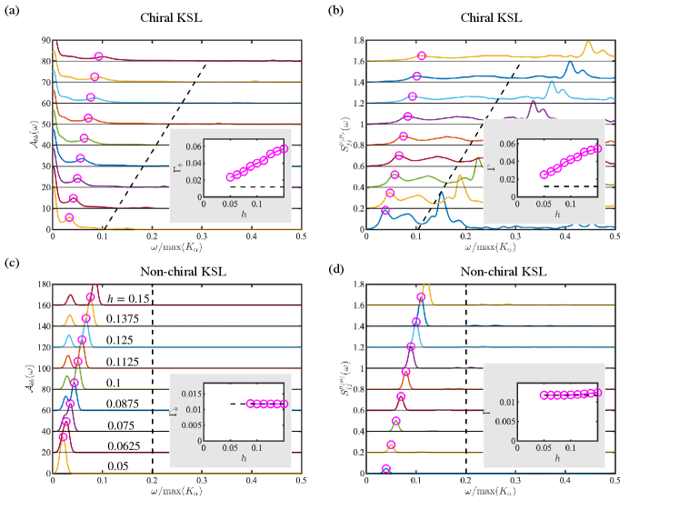
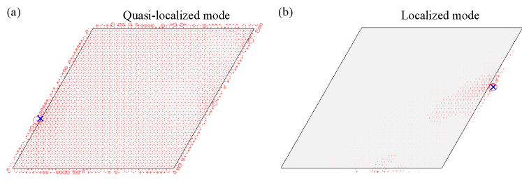
In the presence of disorder, develops a series of peaks superimposed on a continuum background, as shown in Fig. 5(a) for disorder strength . Importantly, a persistent peak always appears around zero energy, originating from the quasi-flat mode at of the clean boundary. In contrast, the finite-energy peaks appear at different energies depending on the location along the boundary, and correspond to resonances with intrinsic broadening due to the linear-in- hybridization with the chiral boundary mode. Indeed, by fitting these peaks using a Gaussian function, we find that the peak width increases linearly with , as shown in the inset of Fig. 5(a). The real-space wave functions of the corresponding resonance modes are peaked at the location where the given Majorana fermion is excited but extend across the entire lattice [see Fig. 6(a)]. It is important to distinguish the broadening discussed above from the one caused by coupling with the bulk modes. The latter occurs above the bulk gap indicated by the black dashed line in Fig. 5(a).
Next, we discuss the local DSSF at a boundary site, which is the convolution of two Majorana-fermion spectral functions [see Eq. (19)]. As shown in Fig. 5(b), the main features of the local DSSF can still be captured by the convolution involving the narrow -peak in around zero energy, similar to the first term in Eq. (38) for a clean boundary. Therefore, the local DSSF is approximately proportional to , whose structure is similar to that of . This particular convolution gives rise to peaks around the same positions as in the Majorana-fermion spectral function. Notably, the peak width in the local DSSF is well above the energy resolution used in the calculation and increases linearly with . Note that there are additional peaks originating from the convolution of two finite-energy resonance modes, which could be above the bulk gap. For these peaks, however, it is hard to distinguish the broadening due to the chiral boundary mode and that due to the bulk modes since the dangling fermions couple to both of them through the same Zeeman term. Therefore, for the purpose of detecting the chiral boundary mode, one must focus on the structure of the DSSF below the bulk gap.
It is also worth mentioning that a finite-energy resonance mode already appears around a corner of the lattice, i.e., the intersection of two zigzag boundaries [see Fig. 6(a)] in the absence of disorder. The convolution of the zero-energy peak in with this “corner mode” leads to an extra peak in the local DSSF.
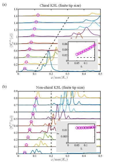
The calculation above assumes that STM has atomic-scale spatial resolution. In a real experiment, however, the effective tip resolution spans a few lattice sites. To account for a finite tip size, we average the local DSSF over five adjacent boundary sites. As shown in Fig. 7(a), we find that the resonance peaks remain resolved for disorder strength . Moreover, both the peak position and the peak width continue to exhibit linear scaling with the field . We finally note that, by averaging over progressively more boundary sites, one eventually crosses over into the disorder-averaged regime discussed in the companion paper [53], where the resonance peaks corresponding to different boundary positions coalesce into a single peak that continues to exhibit linear energy scaling.
IV.2 Non-chiral Kitaev spin liquid
To contrast with the chiral KSL, we next consider the non-chiral KSL. Following the same approach, we first examine the Majorana-fermion spectral functions. Similar to the chiral case, displays several peaks at discrete energy levels, as shown in Fig. 5(c). Unlike in the chiral case, however, these peaks do not exhibit any intrinsic broadening. Instead, the Gaussian fit indicates that the peak width is determined solely by the energy resolution used in the calculation, meaning that the peak width remains constant as a function of , as long as the energy is below the bulk gap. We also observe that the wave functions of the corresponding modes are localized in real space, as illustrated in Fig. 6(b).
Figure 5(c) corresponds to the relative boundary orientation shown in Fig. 3(c), in which case there is a gapless boundary mode in the clean boundary limit. Upon introducing disorder, this gapless boundary mode becomes localized, giving rise to peaks in near zero energy. In contrast, for the alternative boundary considered in Fig. 3(b), where the boundary modes are gapped in the clean boundary limit, the localized modes only appear at finite energy. However, this distinction does not produce observable differences in the local DSSF.
The convolution of these localized boundary modes in the Majorana-fermion spectral function results in a series of discrete -peaks in the local DSSF. The energies of these peaks are found by summing the energies of any two distinct -peaks in the Majorana-fermion spectral function, in accordance with the Pauli exclusion principle. Therefore, the local DSSF shown in Fig. 5(d) does not exhibit a peak around zero energy.
As the field strength increases, the energies of these modes rise linearly, while their peak widths remain constant, determined solely by the energy resolution (i.e., the imaginary part of the complex frequency ) used in the calculation. This behavior in the non-chiral case is clearly distinct from the chiral case, where the peak width increases linearly with the field strength. Moreover, we confirm that this distinction remains observable after averaging over multiple lattice sites within the effective tip size [see Fig. 7(b)]. Finally, the “corner mode” mentioned earlier becomes a truly localized mode for the non-chiral KSL, which implies that its convolution with any other mode localized due to disorder results in an additional -peak in the local DSSF.
V Discussion
Diagnosing quantum spin liquids in real materials is a generally difficult endeavor. For chiral spin liquids, one can exploit the existence of a zero-energy chiral boundary mode, which in principle could be detected through anomalous thermal transport measurements. However, multiple attempts to apply this strategy to -RuCl3 have shown that disentangling the magnetic and lattice contributions to the thermal Hall conductivity is highly challenging [26, 27, 28, 29, 30, 31, 32, 33, 34].
Therefore, it is natural to look for alternative experimental probes of the chiral boundary mode. Recent advances in STM enable real-space spin spectroscopy, allowing experimentalists to directly observe spin excitations at the boundaries of 2D materials. However, as we discuss in this work, the boundary may also host other low-energy excitations, which can occur even in non-chiral spin liquids. Thus, it is crucial to distinguish between cases where only these boundary modes are present and those where they coexist with a chiral boundary mode.
In the specific case of Kitaev spin liquids, the additional low-energy modes arise from dangling Majorana fermions, which hybridize with the chiral boundary mode whenever the KSL is chiral. The presence of a topologically protected chiral boundary mode can then be detected by exploiting its resistance to localization in the presence of boundary disorder. This topological obstruction to Anderson localization is transferred to the additional boundary modes once they hybridize with the chiral boundary mode. Specifically, the disorder-induced localized boundary modes, which exist already in the absence of the topologically protected chiral mode, become resonances when the chiral mode is present. Since the width of each resonance is proportional to the hybridization, which in turn is linear in the applied magnetic field, the presence of the chiral mode can be detected by verifying that both the positions and the widths of the low-energy resonances scale linearly with the external magnetic field.
We conclude that STM is one of the most promising experimental probes for identifying chiral spin liquids. Since its effective spatial resolution allows for probing magnetic atoms on scales smaller than 10 nm—with potential further improvements through enhanced tip quality and optimized experimental conditions—we expect this technique to play a crucial role in diagnosing quantum spin liquids in real materials.
VI Data Availability
The datasets generated during and/or analyzed during the current study are available from the corresponding author upon reasonable request.
VII Code Availability
The codes used during the current study are available from the corresponding author upon reasonable request.
Acknowledgments
SSZ thanks Ruixing Zhang for enlightening discussions. This material is based upon work supported by the U.S. Department of Energy, Office of Science, National Quantum Information Science Research Centers, Quantum Science Center.
VIII Author Contributions
References
- Kitaev [2006] A. Kitaev, Anyons in an exactly solved model and beyond, Annals of Physics 321, 2 (2006), january Special Issue.
- Jackeli and Khaliullin [2009] G. Jackeli and G. Khaliullin, Mott insulators in the strong spin-orbit coupling limit: From heisenberg to a quantum compass and kitaev models, Phys. Rev. Lett. 102, 017205 (2009).
- Rau et al. [2016] J. G. Rau, E. K.-H. Lee, and H.-Y. Kee, Spin-orbit physics giving rise to novel phases in correlated systems: Iridates and related materials, Annual Review of Condensed Matter Physics 7, 195 (2016), https://doi.org/10.1146/annurev-conmatphys-031115-011319 .
- Trebst [2017] S. Trebst, Kitaev Materials, ArXiv e-prints (2017), arXiv:1701.07056 [cond-mat.str-el] .
- Hermanns et al. [2018] M. Hermanns, I. Kimchi, and J. Knolle, Physics of the kitaev model: Fractionalization, dynamic correlations, and material connections, Annual Review of Condensed Matter Physics 9, 17 (2018), https://doi.org/10.1146/annurev-conmatphys-033117-053934 .
- Takagi et al. [2019] H. Takagi, T. Takayama, G. Jackeli, G. Khaliullin, and S. E. Nagler, Concept and realization of kitaev quantum spin liquids, Nature Reviews Physics 1, 264 (2019).
- Singh and Gegenwart [2010] Y. Singh and P. Gegenwart, Antiferromagnetic mott insulating state in single crystals of the honeycomb lattice material , Phys. Rev. B 82, 064412 (2010).
- Liu et al. [2011] X. Liu, T. Berlijn, W.-G. Yin, W. Ku, A. Tsvelik, Y.-J. Kim, H. Gretarsson, Y. Singh, P. Gegenwart, and J. P. Hill, Long-range magnetic ordering in na2iro3, Phys. Rev. B 83, 220403 (2011).
- Choi et al. [2012] S. K. Choi, R. Coldea, A. N. Kolmogorov, T. Lancaster, I. I. Mazin, S. J. Blundell, P. G. Radaelli, Y. Singh, P. Gegenwart, K. R. Choi, S.-W. Cheong, P. J. Baker, C. Stock, and J. Taylor, Spin waves and revised crystal structure of honeycomb iridate , Phys. Rev. Lett. 108, 127204 (2012).
- Ye et al. [2012] F. Ye, S. Chi, H. Cao, B. C. Chakoumakos, J. A. Fernandez-Baca, R. Custelcean, T. F. Qi, O. B. Korneta, and G. Cao, Direct evidence of a zigzag spin-chain structure in the honeycomb lattice: A neutron and x-ray diffraction investigation of single-crystal na2iro3, Phys. Rev. B 85, 180403 (2012).
- Comin et al. [2012] R. Comin, G. Levy, B. Ludbrook, Z.-H. Zhu, C. N. Veenstra, J. A. Rosen, Y. Singh, P. Gegenwart, D. Stricker, J. N. Hancock, D. van der Marel, I. S. Elfimov, and A. Damascelli, as a novel relativistic mott insulator with a 340-mev gap, Phys. Rev. Lett. 109, 266406 (2012).
- Hwan Chun et al. [2015] S. Hwan Chun, J.-W. Kim, J. Kim, H. Zheng, C. C. Stoumpos, C. D. Malliakas, J. F. Mitchell, K. Mehlawat, Y. Singh, Y. Choi, T. Gog, A. Al-Zein, M. M. Sala, M. Krisch, J. Chaloupka, G. Jackeli, G. Khaliullin, and B. J. Kim, Direct evidence for dominant bond-directional interactions in a honeycomb lattice iridate Na2IrO3, Nat. Phys. 11, 462 (2015).
- Singh et al. [2012] Y. Singh, S. Manni, J. Reuther, T. Berlijn, R. Thomale, W. Ku, S. Trebst, and P. Gegenwart, Relevance of the heisenberg-kitaev model for the honeycomb lattice iridates , Phys. Rev. Lett. 108, 127203 (2012).
- Williams et al. [2016] S. C. Williams, R. D. Johnson, F. Freund, S. Choi, A. Jesche, I. Kimchi, S. Manni, A. Bombardi, P. Manuel, P. Gegenwart, and R. Coldea, Incommensurate counterrotating magnetic order stabilized by kitaev interactions in the layered honeycomb , Phys. Rev. B 93, 195158 (2016).
- Kitagawa et al. [2018] K. Kitagawa, T. Takayama, Y. Matsumoto, A. Kato, R. Takano, Y. Kishimoto, R. Dinnebier, G. Jackeli, and H. Takagi, A spin-orbital-entangled quantum liquid on a honeycomb lattice, Nature 554, 341 (2018).
- Bahrami et al. [2019] F. Bahrami, W. Lafargue-Dit-Hauret, O. I. Lebedev, R. Movshovich, H.-Y. Yang, D. Broido, X. Rocquefelte, and F. Tafti, Thermodynamic evidence of proximity to a kitaev spin liquid in , Phys. Rev. Lett. 123, 237203 (2019).
- Plumb et al. [2014] K. W. Plumb, J. P. Clancy, L. J. Sandilands, V. V. Shankar, Y. F. Hu, K. S. Burch, H.-Y. Kee, and Y.-J. Kim, : A spin-orbit assisted mott insulator on a honeycomb lattice, Phys. Rev. B 90, 041112 (2014).
- Sandilands et al. [2015] L. J. Sandilands, Y. Tian, K. W. Plumb, Y.-J. Kim, and K. S. Burch, Scattering continuum and possible fractionalized excitations in , Phys. Rev. Lett. 114, 147201 (2015).
- Sears et al. [2015] J. A. Sears, M. Songvilay, K. W. Plumb, J. P. Clancy, Y. Qiu, Y. Zhao, D. Parshall, and Y.-J. Kim, Magnetic order in : A honeycomb-lattice quantum magnet with strong spin-orbit coupling, Phys. Rev. B 91, 144420 (2015).
- Majumder et al. [2015] M. Majumder, M. Schmidt, H. Rosner, A. A. Tsirlin, H. Yasuoka, and M. Baenitz, Anisotropic magnetism in the honeycomb system: Susceptibility, specific heat, and zero-field nmr, Phys. Rev. B 91, 180401 (2015).
- Johnson et al. [2015] R. D. Johnson, S. C. Williams, A. A. Haghighirad, J. Singleton, V. Zapf, P. Manuel, I. I. Mazin, Y. Li, H. O. Jeschke, R. Valentí, and R. Coldea, Monoclinic crystal structure of and the zigzag antiferromagnetic ground state, Phys. Rev. B 92, 235119 (2015).
- Sandilands et al. [2016] L. J. Sandilands, Y. Tian, A. A. Reijnders, H.-S. Kim, K. W. Plumb, Y.-J. Kim, H.-Y. Kee, and K. S. Burch, Spin-orbit excitations and electronic structure of the putative kitaev magnet , Phys. Rev. B 93, 075144 (2016).
- Banerjee et al. [2016] A. Banerjee, C. A. Bridges, J.-Q. Yan, A. A. Aczel, L. Li, M. B. Stone, G. E. Granroth, M. D. Lumsden, Y. Yiu, J. Knolle, S. Bhattacharjee, D. L. Kovrizhin, R. Moessner, D. A. Tennant, M. D. G., and S. E. Nagler, Proximate Kitaev quantum spin liquid behaviour in a honeycomb magnet, Nature materials 10.1038/nmat4604 (2016).
- Banerjee et al. [2017] A. Banerjee, J. Yan, J. Knolle, C. A. Bridges, M. B. Stone, M. D. Lumsden, D. G. Mandrus, D. A. Tennant, R. Moessner, and S. E. Nagler, Neutron scattering in the proximate quantum spin liquid ?-rucl3, Science 356, 1055 (2017).
- Do et al. [2017] S.-H. Do, S.-Y. Park, J. Yoshitake, J. Nasu, Y. Motome, Y. S. Kwon, D. T. Adroja, D. J. Voneshen, K. Kim, T.-H. Jang, J.-H. Park, K.-Y. Choi, and S. Ji, Majorana fermions in the kitaev quantum spin system î±-rucl3, Nature Physics 13, 1079 (2017).
- Kasahara et al. [2018] Y. Kasahara, T. Ohnishi, Y. Mizukami, O. Tanaka, S. Ma, K. Sugii, N. Kurita, H. Tanaka, J. Nasu, Y. Motome, T. Shibauchi, and Y. Matsuda, Majorana quantization and half-integer thermal quantum hall effect in a kitaev spin liquid, Nature 559, 227 (2018).
- Yamashita et al. [2020] M. Yamashita, J. Gouchi, Y. Uwatoko, N. Kurita, and H. Tanaka, Sample dependence of half-integer quantized thermal hall effect in the kitaev spin-liquid candidate , Phys. Rev. B 102, 220404 (2020).
- Yokoi et al. [2021] T. Yokoi, S. Ma, Y. Kasahara, S. Kasahara, T. Shibauchi, N. Kurita, H. Tanaka, J. Nasu, Y. Motome, C. Hickey, S. Trebst, and Y. Matsuda, Half-integer quantized anomalous thermal hall effect in the kitaev material candidate α-rucl<sub>3</sub>, Science 373, 568 (2021), https://www.science.org/doi/pdf/10.1126/science.aay5551 .
- Lefrançois et al. [2022] E. Lefrançois, G. Grissonnanche, J. Baglo, P. Lampen-Kelley, J.-Q. Yan, C. Balz, D. Mandrus, S. E. Nagler, S. Kim, Y.-J. Kim, N. Doiron-Leyraud, and L. Taillefer, Evidence of a phonon hall effect in the kitaev spin liquid candidate -rucl3, Phys. Rev. X 12, 021025 (2022).
- Kasahara et al. [2022] Y. Kasahara, S. Suetsugu, T. Asaba, S. Kasahara, T. Shibauchi, N. Kurita, H. Tanaka, and Y. Matsuda, Quantized and unquantized thermal hall conductance of the kitaev spin liquid candidate -rucl3, Phys. Rev. B 106, L060410 (2022).
- Bruin et al. [2022] J. A. N. Bruin, R. R. Claus, Y. Matsumoto, N. Kurita, H. Tanaka, and H. Takagi, Robustness of the thermal hall effect close to half-quantization in -rucl3, Nature Physics 18, 401 (2022).
- Czajka et al. [2023] P. Czajka, T. Gao, M. Hirschberger, P. Lampen-Kelley, A. Banerjee, N. Quirk, D. G. Mandrus, S. E. Nagler, and N. P. Ong, Planar thermal hall effect of topological bosons in the kitaev magnet -rucl3, Nature Materials 22, 36 (2023).
- Zhang et al. [2023] H. Zhang, A. F. May, H. Miao, B. C. Sales, D. G. Mandrus, S. E. Nagler, M. A. McGuire, and J. Yan, Sample-dependent and sample-independent thermal transport properties of , Phys. Rev. Mater. 7, 114403 (2023).
- Imamura et al. [2024] K. Imamura, S. Suetsugu, Y. Mizukami, Y. Yoshida, K. Hashimoto, K. Ohtsuka, Y. Kasahara, N. Kurita, H. Tanaka, P. Noh, J. Nasu, E.-G. Moon, Y. Matsuda, and T. Shibauchi, Majorana-fermion origin of the planar thermal hall effect in the kitaev magnet α-rucl<sub>3</sub>, Science Advances 10, eadk3539 (2024), https://www.science.org/doi/pdf/10.1126/sciadv.adk3539 .
- Lambe and Jaklevic [1968] J. Lambe and R. C. Jaklevic, Molecular vibration spectra by inelastic electron tunneling, Phys. Rev. 165, 821 (1968).
- Tsui et al. [1971] D. C. Tsui, R. E. Dietz, and L. R. Walker, Multiple magnon excitation in nio by electron tunneling, Phys. Rev. Lett. 27, 1729 (1971).
- Klein et al. [2018] D. R. Klein, D. MacNeill, J. L. Lado, D. Soriano, E. Navarro-Moratalla, K. Watanabe, T. Taniguchi, S. Manni, P. Canfield, J. Fernández-Rossier, and P. Jarillo-Herrero, Probing magnetism in 2d van der waals crystalline insulators via electron tunneling, Science 360, 1218 (2018).
- Ghazaryan et al. [2018] D. Ghazaryan, M. T. Greenaway, Z. Wang, V. H. Guarochico-Moreira, I. J. Vera-Marun, J. Yin, Y. Liao, S. V. Morozov, O. Kristanovski, A. I. Lichtenstein, M. I. Katsnelson, F. Withers, A. Mishchenko, L. Eaves, A. K. Geim, K. S. Novoselov, and A. Misra, Magnon-assisted tunnelling in van der waals heterostructures based on crbr3, Nature Electronics 1, 344 (2018).
- Kim et al. [2019] H. H. Kim, B. Yang, S. Li, S. Jiang, C. Jin, Z. Tao, G. Nichols, F. Sfigakis, S. Zhong, C. Li, S. Tian, D. G. Cory, G.-X. Miao, J. Shan, K. F. Mak, H. Lei, K. Sun, L. Zhao, and A. W. Tsen, Evolution of interlayer and intralayer magnetism in three atomically thin chromium trihalides, Proceedings of the National Academy of Sciences 116, 11131 (2019).
- Balashov et al. [2006] T. Balashov, A. F. Takács, W. Wulfhekel, and J. Kirschner, Magnon excitation with spin-polarized scanning tunneling microscopy, Phys. Rev. Lett. 97, 187201 (2006).
- Spinelli et al. [2014] A. Spinelli, B. Bryant, F. Delgado, J. Fernández-Rossier, and A. F. Otte, Imaging of spin waves in atomically designed nanomagnets, Nature Materials 13, 782 (2014).
- Delgado et al. [2013] F. Delgado, C. D. Batista, and J. Fernández-Rossier, Local probe of fractional edge states of heisenberg spin chains, Phys. Rev. Lett. 111, 167201 (2013).
- Costa et al. [2020] A. T. Costa, D. L. R. Santos, N. M. R. Peres, and J. Fernández-Rossier, Topological magnons in cri3 monolayers: an itinerant fermion description, 2D Materials 7, 045031 (2020).
- Yin et al. [2020] J.-X. Yin, N. Shumiya, Y. Jiang, H. Zhou, G. Macam, H. O. M. Sura, S. S. Zhang, Z.-J. Cheng, Z. Guguchia, Y. Li, Q. Wang, M. Litskevich, I. Belopolski, X. P. Yang, T. A. Cochran, G. Chang, Q. Zhang, Z.-Q. Huang, F.-C. Chuang, H. Lin, H. Lei, B. M. Andersen, Z. Wang, S. Jia, and M. Z. Hasan, Spin-orbit quantum impurity in a topological magnet, Nature Communications 11, 4415 (2020).
- Yang et al. [2023] B. Yang, Y. M. Goh, S. H. Sung, G. Ye, S. Biswas, D. A. S. Kaib, R. Dhakal, S. Yan, C. Li, S. Jiang, F. Chen, H. Lei, R. He, R. ValentÃÂ, S. M. Winter, R. Hovden, and A. W. Tsen, Magnetic anisotropy reversal driven by structural symmetry-breaking in monolayer î±-rucl3, Nature Materials 22, 50 (2023).
- Feldmeier et al. [2020] J. Feldmeier, W. Natori, M. Knap, and J. Knolle, Local probes for charge-neutral edge states in two-dimensional quantum magnets, Phys. Rev. B 102, 134423 (2020).
- König et al. [2020] E. J. König, M. T. Randeria, and B. Jäck, Tunneling spectroscopy of quantum spin liquids, Phys. Rev. Lett. 125, 267206 (2020).
- Bauer et al. [2023] T. Bauer, L. R. D. Freitas, R. G. Pereira, and R. Egger, Scanning tunneling spectroscopy of majorana zero modes in a kitaev spin liquid, Phys. Rev. B 107, 054432 (2023).
- Takahashi et al. [2023] M. O. Takahashi, M. G. Yamada, M. Udagawa, T. Mizushima, and S. Fujimoto, Nonlocal spin correlation as a signature of ising anyons trapped in vacancies of the kitaev spin liquid, Phys. Rev. Lett. 131, 236701 (2023).
- Kao et al. [2024a] W.-H. Kao, N. B. Perkins, and G. B. Halász, Vacancy spectroscopy of non-abelian kitaev spin liquids, Phys. Rev. Lett. 132, 136503 (2024a).
- Kao et al. [2024b] W.-H. Kao, G. B. Halász, and N. B. Perkins, Dynamics of vacancy-induced modes in the non-abelian kitaev spin liquid, Phys. Rev. B 109, 125150 (2024b).
- Kao et al. [2021] W.-H. Kao, J. Knolle, G. B. Halász, R. Moessner, and N. B. Perkins, Vacancy-induced low-energy density of states in the kitaev spin liquid, Phys. Rev. X 11, 011034 (2021).
- Zhang et al. [2024] S.-S. Zhang, C. D. Batista, and G. B. Halász, Low-energy edge signatures of the kitaev spin liquid (2024), arXiv:2410.21388 [cond-mat.str-el] .
- Altland et al. [2015] A. Altland, D. Bagrets, and A. Kamenev, Topology versus anderson localization: Nonperturbative solutions in one dimension, Phys. Rev. B 91, 085429 (2015).
- Micklitz and Altland [2024] T. Micklitz and A. Altland, Topology obstructing anderson localization of light (2024), arXiv:2405.13277 [cond-mat.dis-nn] .
- Park and Rhim [2024] J.-H. Park and J.-W. Rhim, Quasi-localization and wannier obstruction in partially flat bands, Communications Physics 7, 179 (2024).
- Zhang et al. [2021] S.-S. Zhang, G. B. Halász, W. Zhu, and C. D. Batista, Variational study of the kitaev-heisenberg-gamma model, Phys. Rev. B 104, 014411 (2021).
- Song et al. [2016] X.-Y. Song, Y.-Z. You, and L. Balents, Low-energy spin dynamics of the honeycomb spin liquid beyond the kitaev limit, Phys. Rev. Lett. 117, 037209 (2016).
- Anderson [1958] P. W. Anderson, Absence of diffusion in certain random lattices, Phys. Rev. 109, 1492 (1958).