Probing primordial non-Gaussianity with 21 cm fluctuations from minihalos

Introduction.— Primordial non-Gaussianity is one of the most important quantities to probe the inflationary Universe and the origin of density fluctuations. Its existence inevitably indicates an inflationary model beyond the standard single-field inflation such as the existence of multiple fields, noncanonical kinetic term, deviations from the initial Bunch-Davies vacuum and so on (see, e.g., Ref Bartolo:2004if ; Chen:2010xka ; Wands:2010af for reviews and references therein). Non-Gaussianities can be characterized by bispectrum $B$ and trispectrum $T$, which are defined by connected part of three point and four point functions of the primordial curvature perturbation $\Phi(\vec{k})$:

For the case of the so-called local-type non-Gaussianity, we can expand $\Phi$ as Komatsu:2001rj

and the bispectrum and the trispectrum are given by

where $P_{\Phi}(k)$ is the power spectrum of Gaussian part of $\Phi$ and $k_{13}\equiv\left|\vec{k}_{1}+\vec{k}_{3}\right|$. The parameters $f_{\rm NL}$ and $g_{\rm NL}$ correspond to the amplitude of bispectrum $B$ and trispectrum $T$ normalized by $P_{\Phi}^{2}$ and $P_{\Phi}^{3}$, respectively. Besides, $\tau_{\rm NL}$ is another parameter which characterizes the size of the trispectrum for a different configuration of wave numbers.

To date, cosmic microwave background (CMB) observations give the most severe constraint on non-Gaussianities. The current best constraints on $f_{\rm NL}$ and $g_{\rm NL}$ are given by the Planck 2015 result as $f_{\rm NL}=0.8\pm 5.0$ and $g_{\rm NL}=(9.0\pm 7.7)\times 10^{4}$ at 1$\sigma$ Ade:2015ava , whilst the one for $\tau_{\rm NL}$ is given as $\tau_{\rm NL}\leq 2800$ at 95% C.L. by the Planck 2013 result Ade:2013ydc . Although the constraint on $f_{\rm NL}$ is relatively severe, the ones for the trispectrum, $\tau_{\rm NL}$ and $g_{\rm NL}$, are rather weak and do not give meaningful information for models of the inflationary Universe. However, the trispectrum is potentially very important to differentiate inflationary models since they provide a consistency check of the models. In fact, when the source of primordial fluctuations originates from a single field, $\tau_{\rm NL}$ in Eq. (5) is related to $f_{\rm NL}$ by $\tau_{\rm NL}=(36/25)f_{\rm NL}^{2}$ Boubekeur:2005fj . However, on the other hand, when primordial fluctuations are generated from multiple fields, the above relation becomes an inequality $\tau_{\rm NL}\geq(36/25)f_{\rm NL}^{2}$, which is the so-called Suyama-Yamaguchi inequality Suyama:2007bg , and this inequality has been shown to be valid under a quite general assumption Smith:2011if ; Assassi:2012zq which are satisfied in almost all models of primordial fluctuations suggested so far. In any case, the deviation from the relation $\tau_{\rm NL}=(36/25)f_{\rm NL}^{2}$ would give significant implications for the inflationary Universe and hence checking this relation is very important, where the information of the trispectrum is essential. Furthermore, even if the amplitude of the bispectrum $f_{\rm NL}$ is small, the trispectrum can be large in some models Suyama:2010uj ; Suyama:2013rol . In this regard, it would be worth investigating to what extent we can probe the trispectrum in future observations. We in this paper study expected sensitivities for the non-linearity parameters, particularly focusing on $\tau_{\rm NL}$ and $g_{\rm NL}$ from future 21 cm line fluctuations from minihalos by adopting Fisher matrix analysis for its angular power spectrum.

Redshifted 21 cm line emission/absorption is the unique probe of cosmic neutral hydrogen in the dark ages. By observing its fluctuations, we can extract cosmological information from unexplored redshifts with an unprecedented volume Furlanetto:2006jb . Following the recent detection reported by EDGES Bowman , upcoming Square Kilometre Array (SKA) SKA will be measuring the 21 cm fluctuations which is expected to enhance our understanding of the early Universe Blake:2004pb . The feasibility study to constrain the primordial non-Gaussianity parameters through 21 cm observations has been performed with considering the various aspects of 21 cm signatures of the primordial non-Gaussianity Cooray:2006km ; Joudaki:2011sv ; Tashiro:2011br ; Tashiro:2012wr ; Chongchitnan:2012we . In this paper we particularly focus on the 21 cm line fluctuations from the so-called minihalos Iliev:2002gj ; Furlanetto:2002ng ; Sekiguchi:2013lma ; Sekiguchi:2014wfa , which are halos so small that its virial temperature is not high enough to activate star formation inside. While much attention has been paid to the 21 cm fluctuations from smoothed intergalactic medium, minihalos are expected to contribute predominantly at low redshifts near the completion of the cosmic reionization. With its abundance being sensitive to density fluctuations at sub-Mpc scales, 21 cm line fluctuations from minihalos enable us to probe primordial perturbations at a wide range of scales Sekiguchi:2017cdy .

21 cm angular power spectrum from minihalos.— Given a line of sight $\hat{n}$ and a redshift $z$, fluctuations in the differential brightness temperature $\delta\Delta T_{b}(\hat{n},z)$ from minihalos is given by Iliev:2002gj ; Sekiguchi:2013lma ; Sekiguchi:2014wfa

where $\overline{\Delta T_{b}}$ is the mean differential brightness temperature and $\delta_{h}$ is the fractional overdensity in the minihalo number density. Note that, in Eq. (6), we omitted the redshift-space distortion, which will be incorporated shortly later. On large scales, $\delta_{h}$ is linearly related to the matter overdensity $\delta$ in the Fourier space as

where $\beta$ is the effective bias of minihalos with respect to the underlying matter density fluctuations $\delta$. The bias $\beta$ is given by Iliev:2002gj

where $b(k,M,z)$ is the bias of minihalos with mass $M$, $\mathcal{F}(z,M)$ is a flux from a single minihalo and $dn/dM$ is the mass function of minihalos. The halo matter power spectrum can be given by

with $D(z)$ being the growth factor at $z$ normalized to unity at $z=0$, where the the matter power spectrum $P_{\delta\delta}(k)$ is measured.

In the presence of the local-type non-Gaussianity, the local number density of halos is modulated by the long-wavelength fluctuations. This leads to the scale-dependence in the halo bias at very large scale. The deviation in $b(k,M,z)$ (in $\beta(k,z)$) from the Gaussian case is given by Dalal:2007cu ; Matarrese:2008nc ; Slosar:2008hx ; Smith:2011ub ; Gong:2011gx ; Yokoyama:2012az

where $T(k)$ is the transfer function, $\Omega_{m}$ is the density parameter for total matter and $H_{0}$ is the Hubble constant. We use the following expressions for $b_{f}$ and $b_{g}$ Smith:2011ub :

where $\delta_{\rm cr}\simeq 1.67$, $\nu=\delta_{\rm cr}/\sigma$, and we denote the root mean square of matter density fluctuations smoothed over a top-hat volume enclosing mass $M$ by $\sigma$. Here, $b_{0}(M,z)$ is the Gaussian linear bias and $\hat{\kappa}_{3}$ is the (reduced) third order cumulant defined by $f_{\rm NL}\hat{\kappa}_{3}\equiv\langle\delta^{3}\rangle/\sigma^{3}$:

with $W_{M}(k)$ being the window function corresponding to a mass $M$. For the purpose of demonstration, in this paper we adopt the Sheth-Tormen mass function Sheth:1999mn in computing the minihalo abundance and its Gaussian linear bias. Note that here we have neglected effects of the primordial non-Gaussianity on the mean minihalo abundance, because the effects should not be significant Yokoyama:2011sy for the level non-Gaussianity we suppose in this paper.

By taking into account the redshift space distortion at linear level (i.e. the Kaiser effect Kaiser:1987qv ), the fractional overdensity of minihalo abundance in redshift space (denoted with $\delta_{h}^{s}$) is given by

where $f(z)=d\ln D(z)/d\ln a$ and $\mu=\hat{k}\cdot\hat{n}$ is the cosine between $\vec{k}$ and the line of sight $\hat{n}$.

So far, we have been adopting the exact form of Eq. (3) for $\Phi$ and this results in a term proportional to $f_{\rm NL}^{2}$ in the expression of Eq. (9). In general, multiple sources contribute to non-Gaussianity and in such a case one needs to replace $f_{\rm NL}^{2}$ with $({25}/36)\tau_{\rm NL}$. Finally, we obtain the following expression for the minihalo power spectrum in the redshift space as

where $\beta_{0}$, $\beta_{f}$ and $\beta_{g}$ are obtained by replacing $b(k,M,z)$ in Eq. (8) with $b_{0}$, $b_{f}$ and $b_{g}$, respectively. Note that here we have omitted terms proportional to $f_{\rm NL}g_{\rm NL}$ or $g_{\rm NL}^{2}$ since they would give minor contributions.

In the same manner as in Ref. Sekiguchi:2017cdy , we define the tomographic angular power spectrum of the 21cm line fluctuations from minihalos, $C_{l}^{\rm(21cm)}(z,z^{\prime})$ by

Forecasted constraints.— We perform the Fisher matrix analysis to obtain forecasted constraints on $f_{\rm NL},\tau_{\rm NL}$ and $g_{\rm NL}$. Details of the computation of the Fisher matrix of 21 cm line and CMB angular power spectra are provided in our previous paper Sekiguchi:2017cdy . Specifications of surveys adopted in this paper are summarized in Tables 1 Planck:2006aa ; core and 2 SKA ; Tegmark:2008au . In our baseline analysis, the maximum and minimum redshifts where minihalo can be observed are set to $z_{\rm max}=20$ and $z_{\rm min}=6$, respectively. Since $z_{\rm min}$ can sizeably affect the forecasted constraints, we also examine the dependence of our results on $z_{\rm min}$. In addition to the angular power spectra of CMB and 21 cm line, we also include the CMB temperature bispectrum and trispectrum. We compute the CMB Fisher matrix of the non-linearity parameters based on Komatsu:2001rj ; Kogo:2006kh ; Sekiguchi:2013hza , neglecting the correlation between $g_{\rm NL}$ and $\tau_{\rm NL}$ for simplicity.

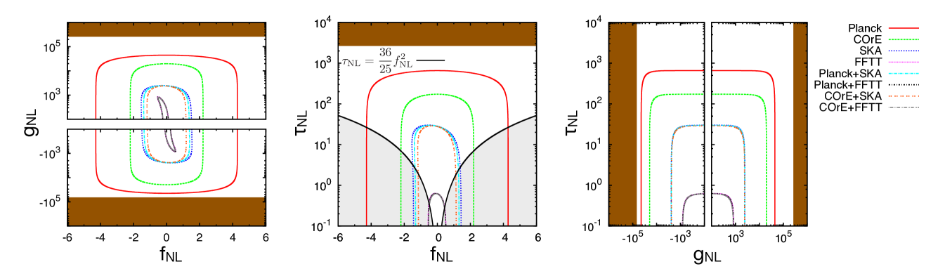
The expected 1$\sigma$ errors based on the Fisher matrix analysis are summarized in Table 3. In Fig. 1, projected constraints are shown on the $f_{\rm NL}$–$g_{\rm NL}$, $f_{\rm NL}$–$\tau_{\rm NL}$ and $g_{\rm NL}$–$\tau_{\rm NL}$ planes. For reference, the current 2$\sigma$ constraints on $\tau_{\rm NL}$ and $g_{\rm NL}$ are also shown by shade for the excluded parameter space. In the $f_{\rm NL}$–$\tau_{\rm NL}$ plane, the line of $\tau_{\rm NL}=(36/25)f_{\rm NL}^{2}$ and the region where the Suyama-Yamaguchi inequality does not hold are also shown. As seen from the figure, future observations of 21 cm angular power spectrum can much improve constraints on the non-linearity parameters, by a few orders of magnitude compared to the current ones. Even compared with future CMB observations, the sensitivity is better already at the level of SKA. With the specification of FFTT, we can obtain unprecedented sensitivities particularly for $\tau_{\rm NL}$ and $g_{\rm NL}$.

In Fig. 2, regions where the consistency relation $\tau_{\rm NL}=(36/25)f_{\rm NL}^{2}$ can be excluded at 1$\sigma$ are shown for COrE, SKA and FFTT alone analysis are shown. For the fiducial values of $f_{\rm NL}$ and $\tau_{\rm NL}$ above each solid line and below each dashed line, we can confirm that the consistency relation does not hold at 1$\sigma$. For reference, we also show predictions of some models (see Suyama:2010uj ; Suyama:2013rol for details of the models) in the same figure.

In Table 4, we summarize the dependence of the constraint on $z_{\rm min}$ in the cases of SKA+Planck and COrE+FFTT. As the reionization proceeds, minihalos start to be ionized by background UV and host stars by molecular hydrogen cooling. Therefore there exists a theoretical uncertainty in the determination of $z_{\rm min}$. However most of minihalos can survive until the late stage of the reionization process ($z\sim 8$) Iliev:2004mb ; Hasegawa:2012uf . We in this paper adopt $z_{\rm min}=6$ as a fiducial value, which could be allowed depending on reionization models.

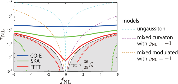
Discussion.— As shown in Table 3, future observations of 21 cm fluctuations can probe the non-linearity parameters, particularly those for trispectrum as $\tau_{\rm NL}\sim 30$ and $g_{\rm NL}\sim 2\times 10^{3}$ for SKA and $\tau_{\rm NL}\sim 0.6$ and $g_{\rm NL}\sim 8\times 10^{2}$ for FFTT. As mentioned in the introduction, some inflationary models can generate a large value of $g_{\rm NL}$ while keeping $f_{\rm NL}$ small Suyama:2010uj ; Suyama:2013rol . Such models can be excluded once we obtain the above level sensitivity in future observations. Moreover, even if $f_{\rm NL}$ and $g_{\rm NL}$ are severely constrained, we still cannot differentiate between single-field and multi-field models. Nevertheless, if we can also probe $\tau_{\rm NL}$ with a good sensitivity, we will be able to test models by looking at the consistency relation: the equality $\tau_{\rm NL}=(36/25)f_{\rm NL}^{2}$ is satisfied for a single-field model, while the inequality $\tau_{\rm NL}>(36/25)f_{\rm NL}^{2}$ holds for multi-field models. As examples of multi-field models, we show the predictions of the $f_{\rm NL}$–$\tau_{\rm NL}$ relation for ungaussiton model Boubekeur:2005fj ; Suyama:2008nt , mixed curvaton and inflaton model Langlois:2004nn ; Lazarides:2004we ; Moroi:2005kz ; Moroi:2005np ; Ichikawa:2008iq and mixed modulated reheating and inflaton model Suyama:2007bg ; Ichikawa:2008ne in Fig. 2. As seen from the figure, SKA can differentiate mixed models when $|f_{\rm NL}|>2$. With the sensitivity of FFTT, even when $f_{\rm NL}<{\cal O}(1)$, we can differentiate multi-field nature of the model.

As demonstrated in this paper, future observations of 21 cm angular power spectrum from minihalo would be a powerful tool to probe primordial non-Gaussianity, especially the trispectrum. By using this probe, we can further elucidate the mechanism of the inflationary Universe.

This work is partially supported by JSPS KAKENHI Grant Number 15K05084 (TT), 17H01131 (TT), 15K17646 (HT), 17H01110 (HT), 15K17659 (SY) JP15H02082 (TS), 18H04339 (TS), 18K03640 (TS), MEXT KAKENHI Grant Number 15H05888 (TT, SY), 18H04356 (SY).

References

- (1) N. Bartolo, E. Komatsu, S. Matarrese and A. Riotto, Phys. Rept. 402, 103 (2004) [astro-ph/0406398].
- (2) X. Chen, Adv. Astron. 2010, 638979 (2010) [arXiv:1002.1416 [astro-ph.CO]].
- (3) D. Wands, Class. Quant. Grav. 27, 124002 (2010) [arXiv:1004.0818 [astro-ph.CO]].
- (4) E. Komatsu and D. N. Spergel, Phys. Rev. D 63, 063002 (2001) doi:10.1103/PhysRevD.63.063002 [astro-ph/0005036].
- (5) P. A. R. Ade et al. [Planck Collaboration], Astron. Astrophys. 594, A17 (2016) [arXiv:1502.01592 [astro-ph.CO]].
- (6) P. A. R. Ade et al. [Planck Collaboration], Astron. Astrophys. 571, A24 (2014) [arXiv:1303.5084 [astro-ph.CO]].
- (7) L. Boubekeur and D. H. Lyth, Phys. Rev. D 73, 021301 (2006) [astro-ph/0504046].
- (8) T. Suyama and M. Yamaguchi, Phys. Rev. D 77, 023505 (2008) [arXiv:0709.2545 [astro-ph]].
- (9) K. M. Smith, M. LoVerde and M. Zaldarriaga, Phys. Rev. Lett. 107, 191301 (2011) [arXiv:1108.1805 [astro-ph.CO]].
- (10) V. Assassi, D. Baumann and D. Green, JCAP 1211, 047 (2012) [arXiv:1204.4207 [hep-th]].
- (11) T. Suyama, T. Takahashi, M. Yamaguchi and S. Yokoyama, JCAP 1012, 030 (2010) [arXiv:1009.1979 [astro-ph.CO]].
- (12) T. Suyama, T. Takahashi, M. Yamaguchi and S. Yokoyama, JCAP 1306, 012 (2013) [arXiv:1303.5374 [astro-ph.CO]].
- (13) S. Furlanetto, S. P. Oh and F. Briggs, Phys. Rept. 433, 181 (2006) [astro-ph/0608032].
- (14) J. D. Bowman, A. E. E. Rogers, R. A. Monsalve, T. J. Mozdzen and N. Mahesh, Nature 555, 67-70 (2018).
- (15) https://www.skatelescope.org
- (16) C. A. Blake, F. B. Abdalla, S. L. Bridle and S. Rawlings, New Astron. Rev. 48, 1063 (2004) [astro-ph/0409278].
- (17) A. Cooray, Phys. Rev. Lett. 97, 261301 (2006) [astro-ph/0610257].
- (18) S. Joudaki, O. Dore, L. Ferramacho, M. Kaplinghat and M. G. Santos, Phys. Rev. Lett. 107, 131304 (2011) [arXiv:1105.1773 [astro-ph.CO]].
- (19) H. Tashiro and N. Sugiyama, Mon. Not. Roy. Astron. Soc. 420, 441 (2012) [arXiv:1104.0149 [astro-ph.CO]].
- (20) H. Tashiro and S. Ho, Mon. Not. Roy. Astron. Soc. 431, 2017 (2013) [arXiv:1205.0563 [astro-ph.CO]].
- (21) S. Chongchitnan and J. Silk, Mon. Not. Roy. Astron. Soc. 426, L21 (2012) [arXiv:1205.6799 [astro-ph.CO]].
- (22) I. T. Iliev, P. R. Shapiro, A. Ferrara and H. Martel, Astrophys. J. 572, 123 (2002) [astro-ph/0202410].
- (23) S. Furlanetto and A. Loeb, Astrophys. J. 579, 1 (2002) [astro-ph/0206308].
- (24) T. Sekiguchi, H. Tashiro, J. Silk and N. Sugiyama, JCAP 1403, 001 (2014) [arXiv:1311.3294 [astro-ph.CO]].
- (25) T. Sekiguchi and H. Tashiro, JCAP 1408, 007 (2014) [arXiv:1401.5563 [astro-ph.CO]].
- (26) T. Sekiguchi, T. Takahashi, H. Tashiro and S. Yokoyama, JCAP 1802, no. 02, 053 (2018) [arXiv:1705.00405 [astro-ph.CO]].
- (27) N. Dalal, O. Dore, D. Huterer and A. Shirokov, Phys. Rev. D 77, 123514 (2008) [arXiv:0710.4560 [astro-ph]].
- (28) S. Matarrese and L. Verde, Astrophys. J. 677, L77 (2008) [arXiv:0801.4826 [astro-ph]].
- (29) A. Slosar, C. Hirata, U. Seljak, S. Ho and N. Padmanabhan, JCAP 0808, 031 (2008) [arXiv:0805.3580 [astro-ph]].
- (30) K. M. Smith, S. Ferraro and M. LoVerde, JCAP 1203, 032 (2012) [arXiv:1106.0503 [astro-ph.CO]].
- (31) J. O. Gong and S. Yokoyama, Mon. Not. Roy. Astron. Soc. 417, 79 (2011) [arXiv:1106.4404 [astro-ph.CO]].
- (32) S. Yokoyama and T. Matsubara, Phys. Rev. D 87, 023525 (2013) [arXiv:1210.2495 [astro-ph.CO]].
- (33) S. Yokoyama, N. Sugiyama, S. Zaroubi and J. Silk, Mon. Not. Roy. Astron. Soc. 417, 1074 (2011) [arXiv:1103.2586 [astro-ph.CO]].
- (34) N. Kaiser, Mon. Not. Roy. Astron. Soc. 227, 1 (1987).
- (35) R. K. Sheth and G. Tormen, Mon. Not. Roy. Astron. Soc. 308, 119 (1999) [astro-ph/9901122].
- (36) S. Chongchitnan and J. Silk, Phys. Rev. D 85, 063508 (2012) [arXiv:1107.5617 [astro-ph.CO]].
- (37) J. Tauber et al. [Planck Collaboration], astro-ph/0604069.
- (38) http://www.core-mission.org
- (39) M. Tegmark and M. Zaldarriaga, Phys. Rev. D 79, 083530 (2009) doi:10.1103/PhysRevD.79.083530 [arXiv:0805.4414 [astro-ph]].
- (40) N. Kogo and E. Komatsu, Phys. Rev. D 73, 083007 (2006) [astro-ph/0602099].
- (41) T. Sekiguchi and N. Sugiyama, JCAP 1309, 002 (2013) [arXiv:1303.4626 [astro-ph.CO]].
- (42) I. T. Iliev, P. R. Shapiro and A. C. Raga, Mon. Not. Roy. Astron. Soc. 361, 405 (2005) [astro-ph/0408408].
- (43) K. Hasegawa and B. Semelin, Mon. Not. Roy. Astron. Soc. 428, 154 (2013) [arXiv:1209.4143 [astro-ph.CO]].
- (44) T. Suyama and F. Takahashi, JCAP 0809, 007 (2008) [arXiv:0804.0425 [astro-ph]].
- (45) D. Langlois and F. Vernizzi, Phys. Rev. D 70, 063522 (2004) [astro-ph/0403258].
- (46) G. Lazarides, R. Ruiz de Austri and R. Trotta, Phys. Rev. D 70, 123527 (2004) [hep-ph/0409335].
- (47) T. Moroi, T. Takahashi and Y. Toyoda, Phys. Rev. D 72, 023502 (2005) [hep-ph/0501007].
- (48) T. Moroi and T. Takahashi, Phys. Rev. D 72, 023505 (2005) [astro-ph/0505339].
- (49) K. Ichikawa, T. Suyama, T. Takahashi and M. Yamaguchi, Phys. Rev. D 78, 023513 (2008) [arXiv:0802.4138 [astro-ph]].
- (50) G. Dvali, A. Gruzinov and M. Zaldarriaga, Phys. Rev. D 69, 023505 (2004) [astro-ph/0303591].
- (51) L. Kofman, astro-ph/0303614.
- (52) K. Ichikawa, T. Suyama, T. Takahashi and M. Yamaguchi, Phys. Rev. D 78, 063545 (2008) [arXiv:0807.3988 [astro-ph]].