∎
e1e-mail: nivaldolemos@id.uff.br \thankstexte2e-mail: dmuller@unb.br \thankstexte3e-mail: reboucas@cbpf.br
Probing time orientability of spacetime
Abstract
In general relativity, cosmology and quantum field theory, spacetime is assumed to be an orientable manifold endowed with a Lorentz metric that makes it spatially and temporally orientable. The question as to whether the laws of physics require these orientability assumptions is ultimately of observational or experimental nature, or the answer might come from a fundamental theory of physics. The possibility that spacetime is time non-orientable lacks investigation, and so should not be dismissed straightaway. In this paper, we argue that it is possible to locally access a putative time non-orientability of Minkowski empty spacetime by physical effects involving quantum vacuum electromagnetic fluctuations. We set ourselves to study the influence of time non-orientability on the stochastic motions of a charged particle subject to these electromagnetic fluctuations in Minkowski spacetime equipped with a time non-orientable topology and with its time orientable counterpart. To this end, we introduce and derive analytic expressions for a statistical time orientability indicator. Then we show that it is possible to pinpoint the time non-orientable topology through an inversion pattern displayed by the corresponding orientability indicator, which is absent when the underlying manifold is time orientable.
pacs:
03.70.+k, 05.40.Jc, 42.50.Lc, 04.20.Gz, 98.80.Jk, 98.80.Cq1 Introduction
In relativistic cosmology and quantum field theory spacetime is described as a four-dimensional differentiable manifold, a topological space with an additional differentiable structure that permits to locally define connections, metric and curvature with which the gravitation theories and the dynamics of other fields are locally formulated. So, two important elements in the mathematical description of the Universe and in the local dynamics of the (micro) physical laws are the geometry and the topology of the underlying spacetime manifold.
Geometry is a local attribute that brings about curvature. Topology is a global property of manifolds that requires consideration of the entire manifold. However, if local physics is brought into the scene, it can play a key role in the local access to the topological properties of spacetime. This is the main concern of this work, which focuses on the time orientability of spacetime.
For a manifold endowed with a Lorentz metric, two possible types of orientability (non-orientability) come about: spatial or temporal orientability (non-orientability), depending on the way the manifold is equipped with a Lorentz metric. Whether a spacetime is time or space orientable may be looked upon as a joint topological-geometrical property, in the sense that it depends on the topology of the underlying manifold but also on the specific Lorentz metric we equip the manifold with Hawking-Ellis-1973 ; Geroch-Horowitz-1979 ; Minguzzi-2019 .
It is generally assumed that the spacetime manifolds one deals with in physics are orientable and endowed with a Lorentz metric, making them separately time and space orientable.111Theoretical arguments in support of these orientability assumptions combine space and time universality of local physical laws with the thermodynamically defined local arrow of time, charge conjugation and parity (CP) violation and CPT invariance Zeldovich1967 ; Hawking-Ellis-1973 ; Geroch-Horowitz-1979 . The impossibility of having globally defined spinor fields on non-orientable spacetime manifolds is also often used in favor of these orientability assumptions Hawking-Ellis-1973 ; Geroch-Horowitz-1979 ; Penrose-1968 ; Penrose-Hindler1986 ; Geroch-1968 ; Geroch-1970 . It should be noted, however, that time universality can be looked upon as a topological assumption of global time homogeneity. This topological assumption rules out time non-orientability from the outset. Non-orientability raises intriguing questions, and it is generally seen as an undesirable feature in physics. Yet, space and time non-orientability of Lorentzian spacetime manifolds are concrete mathematical possibilities for the physical spacetime. On the other hand, strict orientability assumptions could risk ruling out something that the spacetime topology might be trying to “tell” us, and it might also discourage further investigations on the interplay of physics and topology. The answer to questions regarding the orientability of spacetime might come from local experiments, cosmological observations or from a fundamental theory of physics.
In this article we address the question as to whether one can empirically and locally access the putative topological property of time non-orientability (orientability) of spacetime manifolds .222The nature of time and the existence of various arrows of time are contested issues, which we evade in this paper, in which we assume that time is real and passes in all scales. The literature on this debate is fascinating and vast, but for the sake of brevity we refer the readers to Refs. Ellis-Drosel-2020 ; Castagnino-Lara-Lombardi-2003 and references therein, including the books Reichenbach-1971 ; Davies-1974 ; Barbour-2000 ; Rovelli-2018 . Since the net role played by time orientability is more clearly ascertained in static flat spacetime, whose dynamical degrees of freedom are frozen, in this work we focus on Minkowski spacetime. The physical system that turns out to be suitable to play the revealing role of global time non-orientability is a non-relativistic charged particle locally subjected to quantum vacuum fluctuations of the electromagnetic field.333 In an influential work, this system was used by Yu and Ford yf04 in Minkowski spacetime with a conducting plane (nontrivial spatial topology). They endeavored to shed light on the question as to whether a test charged particle would perform stochastic motions induced by quantum fluctuations of the electromagnetic field gs99 ; jr92 . Related investigations have since been made in a number of papers, including Refs. Bessa:2019aar ; Yu:2004gs ; Ford:2005rs ; Yu:2006tn ; Seriu:2008 ; Parkinson:2011yx ; DeLorenci:2016jhd ; Lemos:2020ogj ; Lemos-Muller-Reboucas-2022 .
To show that one can access time orientability, we investigate signatures of time non-orientability through the stochastic motions of a charged test particle under electromagnetic quantum fluctuations in Minkowski spacetime with a time non-orientable topology and in its time orientable counterpart. The time orientability statistical indicator that we introduce combines geometrical-topological properties with the dynamics of the above specific physical system engineered to test orientability.
The structure of the paper is as follows. In Section 2 we set up the notation and present some key concepts and results regarding topology of manifolds, which will be needed in the remainder of the paper. In Section 3 we present the physical system along with the background geometry and topology. In Section 4 we introduce the time orientability statistical indicator and derive its expressions for a charged particle under quantum vacuum electromagnetic fluctuations in Minkowski spacetime equipped with temporally non-orientable and orientable topologies. We show that a comparison of the time evolution of our statistical indicators for these cases allows one to discriminate the orientable from the non-orientable topology. Time non-orientability can be locally unveiled by the inversion pattern of the curves of the time orientability statistical indicator for a point charge under quantum vacuum electromagnetic fluctuations. In Section 5 we present our main conclusions and final remarks.
2 Context and mathematical preliminaries
For both the spatially flat Friedmann-Robertson-Walker (FRW) and the Minkowski spacetimes, the underlying manifold is globally decomposable as , where is the simply-connected -manifold . However, the spatial section of both spacetimes can be any quotient manifold of the form , where is the covering space,444 is endowed with the Euclidean metric. and is a discrete group of freely acting isometries of , also referred to as the holonomy Wolf67 ; Thurston . 555Refs. Adams-Shapiro01 ; Cipra02 ; Riazuelo-et-el03 ; Fujii-Yoshii-2011 give a detailed account of the classification of flat -dimensional Euclidean topologies. The familiar form is very often assumed in cosmology and quantum field theory, and in particular it is adopted in cosmic topology, which investigates the spatial topology of the Universe.666For investigations on cosmic topology and recent observational constraints, see Refs. Ellis:1970ey ; LACHIEZEREY1995135 ; Starkman:1998qx ; LEVIN2002251 ; Reboucas:2004dv ; Reboucas-2005 ; Luminet:2016bqv ; 2014 ; 2016 ; Cornish:2003db ; ShapiroKey:2006hm ; Bielewicz:2010bh ; Vaudrevange:2012da ; Aurich:2013fwa ; Gomero:2016lzd .
In the present work we focus on a single topological property of the Minkowski spacetime manifold , namely time orientability. Perhaps the simplest way to equip Minkowski spacetime with time non-orientability is by taking
| (1) |
where is a two-dimensional time non-orientable quotient manifold, , where denotes the simply-connected plane equipped with a Lorentz metric, that is, Minkowski two-dimensional spacetime. It follows that the orientability of reduces to the orientability of .
The simplest example of a two-dimensional Euclidean manifold with nontrivial topology is the cylinder , whose construction as a quotient manifold, , is such that a point of the cylinder is obtained from the covering manifold by identifying the points that are equivalent under the action of the elements of the covering isometry group . Specifically, a point of the cylinder is the equivalence class of all points in the covering space such that , or with being a translation by in the direction of the -axis. A quotient manifold can be visualized by its so-called fundamental domain (cell). The cylinder’s fundamental cell is a strip of bounded by parallel lines, say and , that are identified through translations. The cylinder is a surface lying in three-dimensional space, but this embedded view does not necessarily work for other Euclidean two-manifolds.
The twisted cylinder is an example of manifold that cannot lie in ordinary three-dimensional space without intersecting itself Stillwell-1992 . A point of represents a set of points in the covering space of the form or with being translation by in the -direction followed by an inversion (flip) in the -direction, a single glide reflection. The fundamental cell of the twisted cylinder is a strip of bounded by parallel lines which are identified through a glide reflection: translation followed by a flip (inversion). It should be noticed that the twisted cylinder is often represented by the Möbius strip, which is obtained by identifying two opposite sides of a rectangle after a flip. The twisted cylinder is an infinitely wide Möbius strip. The Möbius strip is visually useful as it can lie in space, but it is not a manifold because it has a boundary. The twisted cylinder, on the other hand, is a genuine quotient manifold but cannot lie in space.
At this point it seems fitting to remark that a quotient manifold is globally homogeneous only if its fundamental cells are identified by translations alone. Therefore, the cylinder is globally homogeneous but the twisted cylinder is not.
Orientability is another very important global (topological) property of a manifold that measures whether one can consistently choose a clockwise orientation for loops in the manifold. A path in that brings a traveler back to the starting point mirror-reversed is called an orientation-reversing path. Manifolds that do not have an orientation-reversing path are called orientable, whereas manifolds that contain an orientation-reversing path are non-orientable Weeks2020 . For two-dimensional quotient manifolds , when the covering group contains at least one isometry that is a reflection (flip) the corresponding quotient manifold is non-orientable. Therefore, the cylinder is orientable but the twisted cylinder is non-orientable.
For the product manifold given by equation (1) to be time non-orientable the factor has to be a Lorentzian non-orientable manifold. It turns out that both the cylinder and the twisted cylinder can be equipped with a Lorentz metric — see Ref. ONeill-1983 , p. 149, Proposition 37. The twisted cylinder is made time non-orientable by endowing it with the Lorentz metric with time as the flipped direction.
3 Charged particle under electromagnetic fluctuations
From now on, we consider a point charge under quantum vacuum electromagnetic fluctuations as the physical system used to locally probe a potential time non-orientablity of spacetime.
3.1 The physical system
Let a nonrelativistic test particle with charge and mass be locally subject to vacuum fluctuations of the electric field in a topologically nontrivial spacetime manifold equipped with the Minkowski metric .
Locally, the motion of the charged test particle is determined by the Lorentz force. In the nonrelativistic limit the equation of motion for the point charge is
| (2) |
where is the particle’s velocity and its position at time . We assume that on the time scales of interest the particle practically does not move, i.e. it has a negligible displacement, so we can ignore the time dependence of . Thus, the particle’s position is taken as constant in what follows yf04 .777The corrections arising from the inexactness of this assumption are negligible in the low velocity regime. Assuming that the particle is initially at rest, integration of Eq. (2) gives
| (3) |
and the mean squared velocity, velocity dispersion or simply dispersion in each of the three independent directions is given by888By definition, .
| (4) |
Following Yu and Ford yf04 , we assume that the electric field is a sum of classical and quantum parts. Because is not subject to quantum fluctuations and , the two-point function in equation (4) involves only the quantum part of the electric field yf04 .
It can be shown bd82 that locally
| (5) | |||||
where, in Minkowski spacetime, the Hadamard function is given by
| (6) |
The subscript indicates standard Minkowski spacetime , and is the spatial separation for topologically trivial Minkowski spacetime:
| (7) |
3.2 The spacetime manifold
| Manifold | Time sep. | Spatial sep. |
|---|---|---|
In this work, the time non-orientable spacetime manifold that we shall consider is of the form in which the first factor is the non-orientable twisted cylinder equipped with a Lorentz metric with time as the flipped coordinate. This makes time non-orientable and, as a consequence, the spacetime manifold is also time non-orientable. In Table 1 we show the time separation and the spatial separation that enter the spacetime interval in for and , the cases treated in this paper. For the non-orientability is associated with the time coordinate.
Let us try to make our terminology and notation as clear as possible. Being aware of the abuse of language but striving for simplicity, we henceforward give the name twisted cylinder, denoted by , to the time non-orientable spacetime with coordinates , whose points are identified as , and equipped with the Lorentz metric , where and are given in the first line of Table 1. Similarly, we give the name cylinder, denoted by , to the time orientable spacetime with coordinates , whose points are identified as , and equipped with the Lorentz metric , where and are given in the second line of Table 1.
4 TIME-ORIENTABILITY INDICATOR FOR THE TWISTED CYLINDER
We take up now the study of the stochastic motions of a charged particle under quantum vacuum electromagnetic fluctuations in the time non-orientable twisted cylinder .
In a topologically nontrivial spacetime, the time interval and the the spatial separation take new forms that capture the periodic boundary conditions imposed on the covering space. To obtain the correlation function for the electric field that is required to compute the velocity dispersion (4) for the twisted cylinder , we replace in Eq. (5) the Hadamard function by its renormalized version given by Bessa:2019aar
| (8) | |||||
where here and in what follows indicates that the Minkowski contribution term is excluded from the summation, and, according to Table 1, the time and space separations for the time non-orientable spacetime are
| (9) |
The infinite sum (8) takes account of the periodicity induced by the cell identification that defines in terms of the covering space. This approach is widely used Dowker-Critchley-1976 ; Dowker-Banach-1978 ; dhi79 ; Gomero-etal ; st06 ; DHO-2001 ; DHO-2002 ; MD-2007 ; Matas and does not mean that local physics is influenced by arbitrarily distant regions that are causally disconnected from the region of interest because the covering space (where the calculations are performed) is not the physical space. The term with in the sum (8) is the Hadamard function for Minkowski spacetime. This term has been subtracted out from the sum because it gives rise to an infinite contribution to the velocity dispersion.
Thus, from equation (5) the renormalized correlation functions
| (10) | |||||
are then given by
| (11) | |||||
where and are given by Eq. (9), while
| (12) |
The orientability indicator that we will consider is defined by replacing the electric field correlation functions in Eq. (4) by their renormalized counterparts:999To avoid a cluttered notation, for the superscript on the statistical indicator and on the electric field correlation functions we write just instead of .
| (13) |
From (8) it is clear that the orientability indicator is the difference between the velocity dispersion in and the one in Minkowski spacetime with trivial topology.
Before moving on to explicit computations, a few words of clarification on the meaning of the indicator (13) are fitting. From equations (4) and (8) a general definition of the orientability indicator can be written in the form
| (14) |
where is the mean square velocity dispersion, and the superscripts and stand for multiply- and simply-connected manifolds, respectively. The right-hand side of (14) is defined by first taking the difference of the two terms with and then setting .
On the face of it, the indicator (14) does not appear to be measurable because it involves the difference of quantities associated with two different spacetimes, but the spacetime we live in is unique. However, is accessible by measurements performed in our spacetime, which is to be tested for time non-orientablity, by the following procedure. First one would measure the velocity correlation function for , then one would subtract out the correlation function that has been theoretically computed for for the corresponding topologically trivial Minkowski spacetime in the Appendix of Ref. Lemos:2020ogj . Finally, the corresponding curve for the difference (14) as a function of time would be plotted in the coincidence limit .101010This approach is analogous to one used in the search for spatial topology of the universe from discrete cosmic sources, called cosmic crystallography LeLaLu , in which a topological signature of space is given by a constant times the difference of the expected pair separation histogram (EPSH), and the EPSH for the underlying simply connected covering manifold GRT01 ; GTRB98 , which can be theoretically computed in analytical form GRT01 ; Reboucas-2000 .
4.1 Indicators for the twisted cylinder
The orientability indicator can be computed with the help of the integrals Bessa:2019aar
| (15) | |||||
and
| (16) | |||||
as well as
| (17) | |||||
and
| (18) | |||||
4.2 Indicators for the cylinder
We are looking for a local way to probe a putative time non-orientability of spacetime. To this end, let us compare the above results for the twisted cylinder manifold with those for its time-orientable counterpart, the cylinder . The indicators for the cylinder are given in Ref. Lemos:2020ogj as111111In equations (26) and (27) of Ref. Lemos:2020ogj the choice was made. Also, what we call here the cylinder is denoted there by .
| (21) | |||
| (22) |
where .
4.3 Locally probing time non-orientability
The time-inversion scale is specified by the topological length scale . In general, the parameter leaves open the scale of time-non-orientability, whose local manifestation is captured by our indicator (13). For example, the parameter can be very small (microscopic) or very large (cosmological). Our calculations hold regardless of its value.
|
|
|---|---|
| (a) | (b) |
The series (19), (21) and (22) are rapidly convergent but we are unable to sum them in closed form. Thus, for the numerical calculations that allow us to produce some figures, we truncate them at .
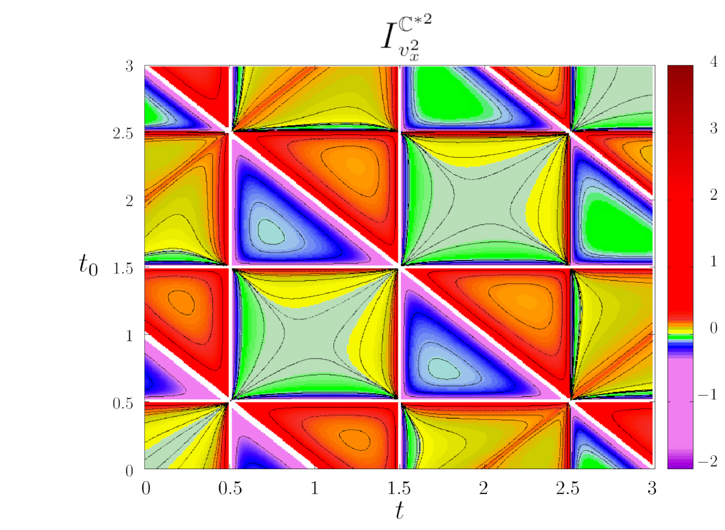
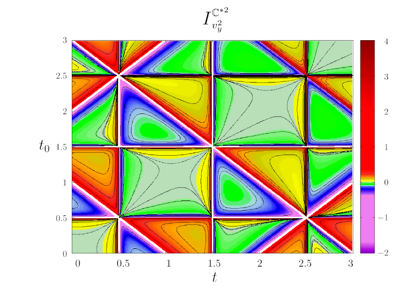
A significant difference between the case of the time non-orientable twisted cylinder and that of time-orientable spacetimes is that the indicator (19) depends both on and , and not only on the difference . This is because the twisted cylinder is not globally temporally homogeneous. By means of a picture, we highlight the main consequences of the twisted cylinder’s lack of global time homogeneity on the statistical indicator (19). In Fig. 1 we show two components of indicator (19) as functions of , with the indicator values represented by colors (the -component of the indicator is not shown because it coincides with its -component). Contour lines of the indicator are also displayed. Figs. 1 (a) and (b) illustrate the global temporal inhomogeneity of the twisted cylinder : the patterns encountered as one moves horizontally along the -axis are different for each fixed . The nontrivial contour curves are also very different from those for , which are the straight lines . There are periodic repetition patterns but with changing absolute value of the indicators. The topological singularity structure, indicated by the white straight lines, is also much richer than the one for the time orientable case. For example, the vertical lines are singularities of topological nature that are not present in the indicators for the time orientable spacetime .
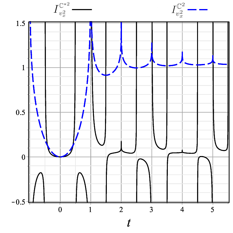
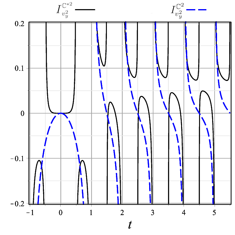
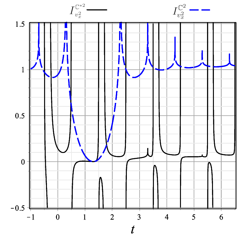
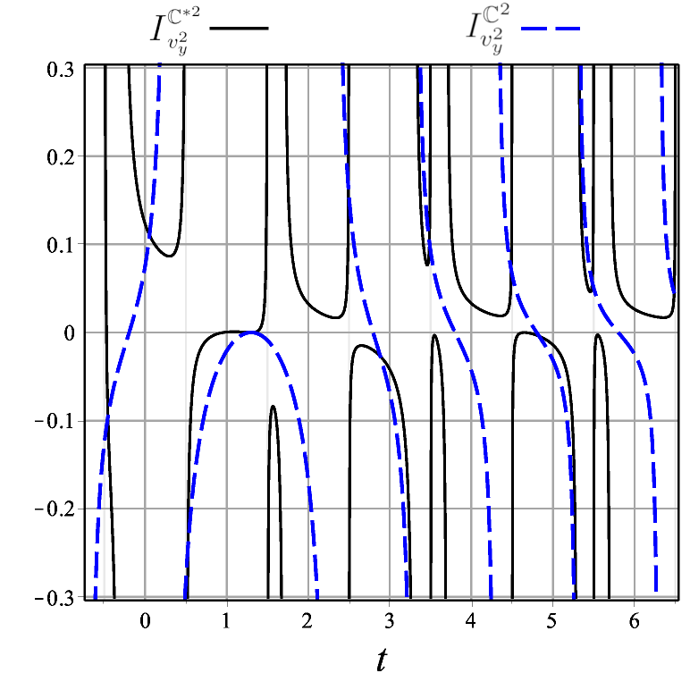
Figure 1 illustrates quite vividly how the global inhomogeneity of the twisted cylinder manifests itself through the statistical indicator (19). Next we study how the indicator (19) for the twisted cylinder behaves as a function of for fixed . Figures 2 and 3 compare components of the indicator for with those for its time orientable counterpart for two values of . Both for (Fig. 2) and (Fig. 3) there appears an inversion pattern in the case of , roughly of the form followed by . The absence of any inversion pattern in the case of the time-orientable allows one to pinpoint the temporally non-orientable case.
In order to demonstrate our main result, namely the possible local detection of time non-orientability, we have chosen two spacetime manifolds of the form such that the first factors are topologically similar in that each is compact in just one direction and has only one discrete isometry generator (see Section II). Thus, the only difference in their construction is that for the cylinder the generator is a translation whereas for the twisted cylinder it is a glide reflection (translation followed by an inversion or flip), which suffices to make the quotient manifold non-orientable. The repeated inversion pattern in the curves for indicator , Eq. (13), for the spacetime manifold with the time non-orientable twisted cylinder factor , constitutes an exclusive signature of time-non-orientability. As for the spacetime manifold with the cylinder factor , the periodic pattern of the curves is uniform (shows no inversion) because is a pure translation isometry. The glide reflection is the only topological difference between the twisted cylinder and the cylinder, therefore it is the cause of the different behaviors of our orientability indicator in the two cases because the physical system is the same.
|
|
|---|---|
| (a) | (b) |
|
|
|---|---|
| (a) | (b) |
4.4 Possible physical realization
A brief discussion of the physical scale in which our approach can be realized is fitting. From Eq. (19), or more clearly from Eq. (21), it follows that the order of magnitude of the time-orientability indicators is
| (23) |
where is the topological length scale and is the measurement duration. The above equation holds in units such that . Let us consider the case in which the charged particle is an electron. Inserting the appropriate factors of and , and using in CGS units, where is the fine-structure constant, we have
| (24) |
which has the correct dimension of velocity squared. Our analysis was performed for nonrelativistic charged particles. Accordingly, for the sake of estimation, let us take . This gives
| (25) |
where we have used , cm/s, g and erg s. Consequently, if then s. This means that it would take no more that a second of observation to detect a possible time non-orientablity in mesoscopic or microscopic scale. The detection time increases proportionally to the cube of the topological length scale. Therefore, the present method would not be suitable for detection of a putative time non-orientablity in the solar system scale, let alone in cosmological scale. Furthermore, for the early expanding universe it is the Friedmann-Lemaître-Robertson-Walker (FLRW) geometry that must be considered, rather than the Minkowski spacetime metric Lemos-Reboucas-2022 .
Our calculations imply that a time non-orientable nontrivial topology will give rise to a certain inversion pattern in the time evolution curves of the statistical orientability indicator. In the case of a time orientable nontrivial topology there will be no such inversion pattern. For trivial topology (standard Minkowski spacetime) the indicator will vanish. In order to decide which of these alternatives is realized in nature, it is necessary to measure stochastic motions of charged particles induced by quantum electromagnetic vacuum fluctuations. Conceivably, experimental detection of such stochastic motions might be feasible for confined electrons in a Paul trapp Matthiesen or in a Penning trap Vogel . It seems likely that technical difficulties will have to be overcome to tell apart the effects induced by quantum electromagnetic vacuum fluctuations from those caused by the applied electromagnetic field that is responsible for the confinement.
5 Summary of results and final comments
In relativistic cosmology and quantum field theory, spacetime is assumed to be orientable as a topological manifold, and is additionally endowed with a Lorentz metric, making it separately time and space orientable. The question as to whether the current laws of physics require that spacetime manifolds adhere to these orientability assumptions are among the unsettled issues in this framework. Although non-orientability is generally seen as an undesirable feature, non-orientable Lorentzian spacetime manifolds are concrete mathematical possibilities in physics at different scales. Therefore, the possibility that spacetime is time non-orientable ought not to be jettisoned forthwith. Strict orientability assumptions could potentially interfere with the understanding of fundamental aspects of the interplay of physics and topology. In fact, we do not know to what extent the topology of the underlying spacetime manifold might encode, or whether it is necessary to capture or express, basic features of the physical world in some scale. It is conceivable that topological properties such as global homogeneity and orientability of spacetime manifolds might be testable in both micro- and macro-physical scales. Previous speculations on time orientability violation have revolved about gedanken experiments that would allegedly provide signatures of a putative time non-orientability of spacetime MarkHadley-2002 ; MarkHadley-2018 . These ideas and other approaches to testing time orientability have been recently subjected to a searching critique Bielinska . Here, however, we have settled on probing the orientability of spacetime by means of measurable local physical effects.
Inasmuch as the role played by time orientability is more clearly accessed in static flat spacetime, whose dynamical degrees of freedom are frozen, in the present paper, instead of the expanding FLRW spacetime, we have focused on the time orientability of Minkowski spacetime, leaving for a forthcoming article Lemos-Reboucas-2022 some important related questions regarding the so-called arrow of time — observed time asymmetry in macrophysics and in the evolution of the universe, despite the time reversal invariance of the fundamental laws of physics. This includes, for example, whether temporal orientability of the FLRW universe can be probed and whether one can understand in a far-reaching context the several existing arrows of time Ellis-Drosel-2020 ; Barbour-2000 ; Rovelli-2018 .
In this paper we have argued that a presumed time non-orientability of Minkowski empty spacetime can be locally probed through physical effects associated with quantum vacuum electromagnetic fluctuations. To this end, we have studied the stochastic motions of a charged particle under these fluctuations in Minkowski spacetime manifold, , endowed with a time non-orientable topology (the twisted cylinder ) and its time orientable counterpart. We have found that the statistical topological indicator given by Eq. (13) is suitable to bring out the time non-orientability in the twisted cylinder case. Accordingly, we have derived analytical expressions for the statistical orientability indicator corresponding to Minkowski spacetime manifold equipped with time non-orienbtable and its time orientable counterpart.
The chief conclusion of this work is reached through comparisons between the stochastic motions of a charged test particle in Minkowski spacetime endowed with each of the two spacetime topologies. Since the expressions for the orientability indicators — Eqs. (19), (21) and (22) — are too involved for a direct comparison, to demonstrate our main result, which is ultimately stated in terms of patterns of curves for the orientability indicators, we have performed numerical computations and plotted figures for the components of our statistical orientability indicator.
Figure 1 aims to illustrate the topological temporal inhomogeneity for corresponding to the twisted cylinder , a feature not shared by the cylinder . The patterns encountered are different for each fixed , and the closed contour curves are also very different from those for , which are straight -degree lines. The topological singularity structure is also markedly richer than the one for the time orientable case.
However, the answer to the central question of the paper, namely how to locally probe the time orientability of Minkowski spacetime intrinsically, is accomplished by comparing the time evolution of the orientability indicators and . Figs. 2 and 3 show that it may be possible to locally unveil time non-orientability through the inversion pattern of curves of the time non-orientability indicator for a charged particle under quantum vacuum electromagnetic fluctuations. This inversion pattern is a signature of time non-orientability and is absent in the time orientable case.
It should be stressed that the time non-orientability for the twisted cylinder is of topological origin (periodic inversion of time controlled by the topological length , the fundamental domain size). It is different from the continuous closed timelike curves that come about in Gödel Godel and other spacetime solutions of Einstein’s equations CTLC-examples ; CTLC-examples-2 ; CTLC-examples-3 ; CTLC-examples-4 ; CTLC-examples-5 . Particularly, in the Gödel model the underlying manifold is topologically equivalent to , there is no periodic time inversion of topological origin, but gravity tilts the local light cones so as to allow continuous closed timelike curves in the topologically trivial spacetime.
To summarize, the main result of our analysis is that it may be feasible to look into a conceivable topological time non-orientability of Minkowski empty spacetime by measurable local physical effects associated with quantum vacuum electromagnetic fluctuations.
Acknowledgements.
M.J. Rebouças acknowledges the support of FAPERJ under a CNE E-26/202.864/2017 grant, and thanks CNPq for the grant under which this work was carried out. We are grateful to A.F.F. Teixeira for a careful reading of the manuscript and discussions.References
- (1)
- (2) S.W. Hawking and G.F.R. Ellis, The Large Scale Structure of Space-Time (Cambridge University Press, Cambridge, 1973).
- (3) R. Geroch and G.T. Horowitz, Global structure of spacetimes in General relativity: An Einstein centenary survey, pp. 212-293, Eds. S. Hawking and W. Israel (Cambridge University Press, Cambridge, 1979).
- (4) E. Minguzzi, Lorentzian causality theory, Living Rev Relativ 22, 3 (2019).
- (5) Ya. B. Zeldovich and I.D. Novikov, JETP Letters 6, 236 (1967).
- (6) R. Penrose, The Structure of Space-Time, in BattelIe Rencontres in Mathematics and Physics: Seattle, 1967, C. M. DeWitt and J. A. Wheeler, Eds. (Benjamin, New York, 1968).
- (7) R. Penrose and W. Rindler, Spinors and Space-time, Volume 1, Two-spinor calculus and relativistic fields (Cambridge University Press, Cambridge, 1986).
- (8) R. Geroch, J. Math. Phys. 9, 1739 (1968).
- (9) R. Geroch, J. Math. Phys. 9, 343 (1970).
- (10) G.F.R. Ellis and B. Drossel, Found. Phys. 50, 161 (2020).
- (11) M. Castagnino, L. Lara and O. Lombardi, Class. Quantum Grav. 20, 369 (2003).
- (12) H. Reichenbach The Direction of Time (University of California Press, Berkeley, 1971).
- (13) P.C.W. Davies, The Physics of Time Asymmetry (University of California Press, Berkeley, 1974).
- (14) J. Barbour, The End of Time: The Next Revolution in Physics (Oxford University Press, Oxford, 2001).
- (15) C. Rovelli, The Order of Time (Riverhead Books, New York, 2018).
- (16) H. Yu and L.H. Ford, Phys. Rev. D 70, 065009 (2004).
- (17) G. Gour and L. Sriramkumar, Found. Phys. 29, 1917 (1999).
- (18) M.T. Jaekel and S. Reynaud, Quant. Opt. 4, 39 (1992).
- (19) C.H.G. Bessa and M.J. Rebouças, Class. Quant. Grav. 37(12), 125006 (2020).
- (20) H.w. Yu and J. Chen, Phys. Rev. D 70, 125006 (2004).
- (21) L.H. Ford, Int. J. Theor. Phys. 44, 1753 (2005).
- (22) H.w. Yu and J. Chen, P.x. Wu, JHEP 02, 058 (2006).
- (23) M. Seriu and C.H. Wu, Physical Review A 77(2) (2008).
- (24) V. Parkinson and L.H. Ford, Phys. Rev. A 84, 062102 (2011).
- (25) V.A. De Lorenci, C.C.H. Ribeiro and M.M. Silva, Phys. Rev. D 94(10), 105017 (2016).
- (26) N.A. Lemos, M.J. Rebouças, Eur. Phys. J. C 81(7), 618 (2021).
- (27) N.A. Lemos, D. Müller and M.J. Rebouças, Phys. Rev. D 106, 023528 (2022)
- (28) J.A. Wolf, Spaces of Constant Curvature (McGraw-Hill, New York, 1967).
- (29) W.P. Thurston, Three-Dimensional Geometry and Topology. Vol.1, Edited by Silvio Levy (Princeton University Press, Princeton, 1997).
- (30) C. Adams and J. Shapiro, American Scientist 89, 443 (2001).
- (31) B. Cipra, What’s Happening in the Mathematical Sciences (American Mathematical Society, Providence, RI, 2002).
- (32) A. Riazuelo, J. Weeks, J.P. Uzan, R. Lehoucq and J.P. Luminet, Phys. Rev. D 69, 103518 (2004).
- (33) H. Fujii and Y. Yoshii, Astron. Astrophys. 529, A121 (2011).
- (34) G.F.R. Ellis, Gen. Rel. Grav. 2, 7 (1971).
- (35) M. Lachièze-Rey and J.P. Luminet, Phys. Rep. 254(3), 135 (1995).
- (36) G.D. Starkman, Class. Quant. Grav. 15, 2529 (1998).
- (37) J. Levin, Phys. Rep. 365(4), 251 (2002).
- (38) M.J. Rebouças and G.I. Gomero, Braz. J. Phys. 34, 1358 (2004).
- (39) M.J. Rebouças, A Brief Introduction to Cosmic Topology, in Proc. XIth Brazilian School of Cosmology and Gravitation, eds. M. Novello and S.E. Perez Bergliaffa (Americal Institute of Physics, Melville, NY, 2005).
- (40) J.P. Luminet, Universe 2(1), 1 (2016).
- (41) P.A.R. Ade, N. Aghanim, C. Armitage-Caplan, M. Arnaud, M. Ashdown, F. Atrio-Barandela, J. Aumont, C. Baccigalupi, A.J. Banday, et al., Astronom. Astrophys. 571, A16 (2014).
- (42) P.A.R. Ade, N. Aghanim, M. Arnaud, M. Ashdown, J. Aumont, C. Baccigalupi, A.J. Banday, R.B. Barreiro, J.G. Bartlett, et al., Astronom. Astrophys. 594, A13 (2016).
- (43) N.J. Cornish, D.N. Spergel, G.D. Starkman and E. Komatsu, Phys. Rev. Lett. 92, 201302 (2004).
- (44) J. Shapiro Key, N.J. Cornish, D.N. Spergel and G.D. Starkman, Phys. Rev. D 75, 084034 (2007).
- (45) P. Bielewicz and A.J. Banday, Mon. Not. Roy. Astron. Soc. 412, 2104 (2011).
- (46) P.M. Vaudrevange, G.D. Starkman, N.J. Cornish and D.N. Spergel, Phys. Rev. D 86, 083526 (2012).
- (47) R. Aurich and S. Lustig, Mon. Not. Roy. Astron. Soc. 433, 2517 (2013).
- (48) G.I. Gomero, B. Mota and M.J. Rebouças, Phys. Rev. D 94(4), 043501 (2016).
- (49) J. Stillwell, Geometry of Surfaces (Springer, New York, 1992).
- (50) J.R. Weeks, The Shape of Space, 3rd ed. (CRC Press, Boca Raton, FL, 2020).
- (51) B. O’Neill, Semi-Riemannian Geometry With Applications to Relativity (Academic Press, New York, 1983).
- (52) N.D. Birrel and P.C.W. Davies, Quantum Fields in Curved Space (Cambridge University Press, Cambridge, 1982).
- (53) J.S. Dowker and R. Critchley, J. Phys. A 9, 535 (1976).
- (54) J. S. Dowker and R. Banach, J. Phys. A: Math. Gen. 11, 2255 (1978).
- (55) B.S. DeWitt, C.F. Hart and C.J. Isham, Physica 96A, 197 (1979).
- (56) G. I. Gomero, M. J. Rebouças, A. F. F. Teixeira and A. Bernui, Int. J. Mod. Phys. A 15, 4141 (2000).
- (57) P.M. Sutter and T. Tanaka, Phys. Rev. D 74, 024023 (2006).
- (58) D. Müller, H.V. Fagundes and R. Opher, Phys. Rev. D 63, 123508 (2001).
- (59) D. Müller, H.V. Fagundes and R. Opher, Phys. Rev. D 66, 083507 (2002).
- (60) M.P. Lima and D. Müller, Class. Quant. Grav. 24, 897 (2007).
- (61) A. Matas, D. Müller and G Starkman, Phys. Rev. D 92, 026005 (2015).
- (62) R. Lehoucq, M. Lachièze-Rey and J.-P. Luminet, Astron. Astrophys. 313, 339 (1996).
- (63) G.I. Gomero, M.J. Rebouças and A.F.F. Teixeira, Class. Quantum Grav. 18, 1885 (2001).
- (64) G.I. Gomero, A.F.F. Teixeira, M.J. Rebouças and A. Bernui, Int. J. Mod. Phys. D 11, 869 (2002).
- (65) M.J. Rebouças, Int. J. Mod. Phys. D 9, 561 (2000).
- (66) C. Matthiesen, Q. Yu, J. Guo, A. M. Alonso, H. Häffner, Phys. Rev. X 11, 011019 (2021) and references therein.
- (67) M. Vogel, Particle Confinement in Penning Traps: An Introduction (Springer, 2018).
- (68) M. Hadley, Class. Quantum Grav. 19, 4565 (2002).
- (69) M. Hadley, Testing the Orientability of Time. Preprints 2018040240 (2018).
- (70) M. Bielińska and J. Read, Found. Phys. 53, 8 (2023).
- (71) N.A. Lemos, D. Müller and M.J. Rebouças (in preparation).
- (72) K. Gödel, Rev. Mod. Phys. 21, 447 (1949).
- (73) W.J. van Stockum, Proc. R. Soc. Edin. 57, 135 (1937).
- (74) M.S. Morris and K.S. Thorne, Am. J. Phys. 56, 395 (1988).
- (75) F.J. Tipler, Phys. Rev. D 9, 2203 (1974).
- (76) J.R. Gott III, Phys. Rev. Lett. 66, 1126 (1991).
- (77) M. Alcubierre, Class. Quant. Grav. 11, L73 (1994).