Projective geometry for blueprints
Abstract.
In this note, we generalize the –construction from usual schemes to blue schemes. This yields the definition of projective space and projective varieties over a blueprint. In particular, it is possible to descend closed subvarieties of a projective space to a canonical –model. We discuss this in case of the Grassmannian .
1. Introduction
Blueprints are a common generalization of commutative (semi)rings and monoids. The associated geometric objects, blue schemes, are therefore a common generalization of usual scheme theory and –geometry (as considered by Kato [5], Deitmar [3] and Connes-Consani [2]). The possibility of forming semiring schemes allows us to talk about idempotent schemes and tropical schemes (cf. [11]). All this is worked out in [9].
It is known, though not covered in literature yet, that the -construction from usual algebraic geometry has an analogue in -geometry (after Kato, Deitmar and Connes-Consani). In this note we describe a generalization of this to blueprints. In private communication, Koen Thas announced a treatment of for monoidal schemes (see [13]).
We follow the notations and conventions of [10]. Namely, all blueprints that appear in this note are proper and with a zero. We remark that the following constructions can be carried out for the more general notion of a blueprint as considered in [9]; the reason that we restrict to proper blueprints with a zero is that this allows us to adopt a notation that is common in -geometry.
Namely, we denote by the (blue) affine -space over a blueprint . In case of a ring, this does not equal the usual affine -space since is not closed under addition. Therefore, we denote the usual affine -space over a ring by . Similarly, we use a superscript “” for the usual projective space and the usual Grassmannian over a ring .
2. Graded blueprints and
Let be a blueprint and a subset of . We say that is additively closed in if for all additive relations with also is an element of . Note that, in particular, is an element of . A graded blueprint is a blueprint together with additively closed subsets for such that , such that for all and , , the product is an element of and such that for every , there are a unique finite subset of and unique non-zero elements for every such that . An element of is called homogeneous. If is non-zero, then we say, more specifically, that is homogeneous of degree .
We collect some immediate facts for a graded blueprint as above. The subset is multiplicatively closed, i.e. can be seen as a subblueprint of . The subblueprint equals if and only if for all , . In this case we say that is trivially graded. By the uniqueness of the decomposition into homogeneous elements, we have for . This means that the union has the structure of a wedge product . Since is multiplicatively closed, it can be seen as a subblueprint of . We define and call the subblueprint the homogeneous part of .
Let be a multiplicative subset of . If is an element of the localization where is homogeneous of degree and is homogeneous of degree , then we say that is a homogeneous element of degree . We define as the subset of homogeneous elements of degree . It is multiplicatively closed, and inherits thus a subblueprint structure from . If is the complement of a prime ideal , then we write for the subblueprint of homogeneous elements of degree in .
An ideal of a graded blueprint is called homogeneous if it is generated by homogeneous elements, i.e. if for every , there are homogeneous elements and elements and an additive relation in .
Let be a graded blueprint. Then we define as the set of all homogeneous prime ideals of that do not contain . The set comes together with the topology that is defined by the basis
where ranges through and with a structure sheaf that is the sheafification of the association where is the localization of at .
Note that if is a ring, the above definitions yield the usual construction of for graded rings. In complete analogy to the case of graded rings, one proves the following theorem.
Theorem 2.1.
The space together with is a blue scheme. The stalk at a point is . If , then . The inclusions yield morphisms , which glue to a structural morphism . ∎
If is a graded blueprint, then the associated semiring inherits a grading. Namely, let the homogeneous part of . Then we can define as the additive closure of in , i.e. as the set of all such that there is an additive relation of the form in with . Then defines a grading of . Similarly, the grading of induces a grading on a tensor product with respect to blueprint morphisms and under the assumption that the image of is contained in . Consequently, a grading of implies a grading of and of the ring . Along the same lines, if both and are graded and the images of and lie in and respectively, then inherits a grading obtained from the gradings of and .
3. Projective space
The functor allows the definition of the projective space over a blueprint . Namely, the free blueprint over comes together with a natural grading (cf. [9, Section 1.12] for the definition of free blueprints). Namely, consists of all monomials such that where . Note that and . The projective space is defined as . It comes together with a structure morphism .
In case of , the projective space is the monoidal scheme that is known from -geometry (see [4], [1, Section 3.1.4]) and [10, Ex. 1.6]). The topological space of is finite. Its points correspond to the homogeneous prime ideals of where ranges through all proper subsets of .
In case of a ring , the projective space does not coincide with the usual projective space since the free blueprint is not a ring, but merely the blueprint of all monomials of the form with . However, the associated scheme coincides with the usual projective space over , which equals .
4. Closed subschemes
Let be a scheme of finite type. By an -model of we mean a blue scheme of finite type such that is isomorphic to . Since a finitely generated -algebra is, by definition, generated by a finitely generated multiplicative subset as a -module, every scheme of finite type has an -model. It is, on the contrary, true that a scheme of finite type possesses a large number of -models.
Given a scheme with an -model , we can associate to every closed subscheme of the following closed subscheme of , which is an -model of . In case that is the spectrum of a blueprint , and thus is an affine scheme, we can define as for where is the pre-addition that contains whenever holds in the coordinate ring of . This is a process that we used already in [10, Section 3].
Since localizations commute with additive closures, i.e. where is a multiplicative subset of , the above process is compatible with the restriction to affine opens . This means that given , which is an -model for , then the –model that is associated to the closed subscheme of by the above process is the spectrum of the blueprint . Consequently, we can associate with every closed subscheme of a scheme with an -model a closed subscheme of , which is an –model of ; namely, we apply the above process to all affine open subschemes of and glue them together, which is possible since additive closures commute with localizations.
In case of a projective variety, i.e. a closed subscheme of a projective space , we derive the following description of the associated -model in by homogeneous coordinate rings. Let be the homogeneous coordinate ring of , which is a quotient of by a homogeneous ideal . Let be the pre-addition on that consists of all relations such that in . Then inherits a grading from by defining as the image of in . Note that and that the sets equal the intersections for where is the homogeneous part of degree of . Then the -model of equals .
5. –models for Grassmannians
One of the simplest examples of projective varieties that is not a toric variety (and in particular, not a projective space) is the Grassmann variety . The problem of finding models over for Grassmann varieties was originally posed by Soulè in [12], and solved by the authors by obtaining a torification from the Schubert cell decomposition (cf. [8, 7]).
In this note, we present -models for Grassmannians as projective varieties defined through (homogeneous) blueprints. The proposed construction for the Grassmannians fits within a more general framework for obtaining blueprints and totally positive blueprints from cluster data (cf. the forthcoming preprint [6]).
Classically, the homogeneous coordinate ring for the Grassmannian is obtained by quotienting out the homogeneous coordinate ring of the projective space by the homogeneous ideal generated by the Plücker relations. A similar construction can be carried out using the framework of (graded) blueprints. In what follows, we make that construction explicit for the Grassmannian .
Define the blueprint where the congruence is generated by the Plücker relation (the signs have been picked to ensure that the totally positive part of the Grassmannian is preserved, cf. [6]). Since is generated by a homogeneous relation, inherits a grading from the canonical morphism
Let . The base extension is the usual Grassmannian, and defines a closed embedding of into , which extends to the classical Plücker embedding .
Homogeneous prime ideals in are described by their generators as the proper subsets such that is either contained in one of the sets , , , or otherwise has a nonempty intersection with all three of them. In other words, cannot contain elements in two of the above sets without also containing an element of the third one.
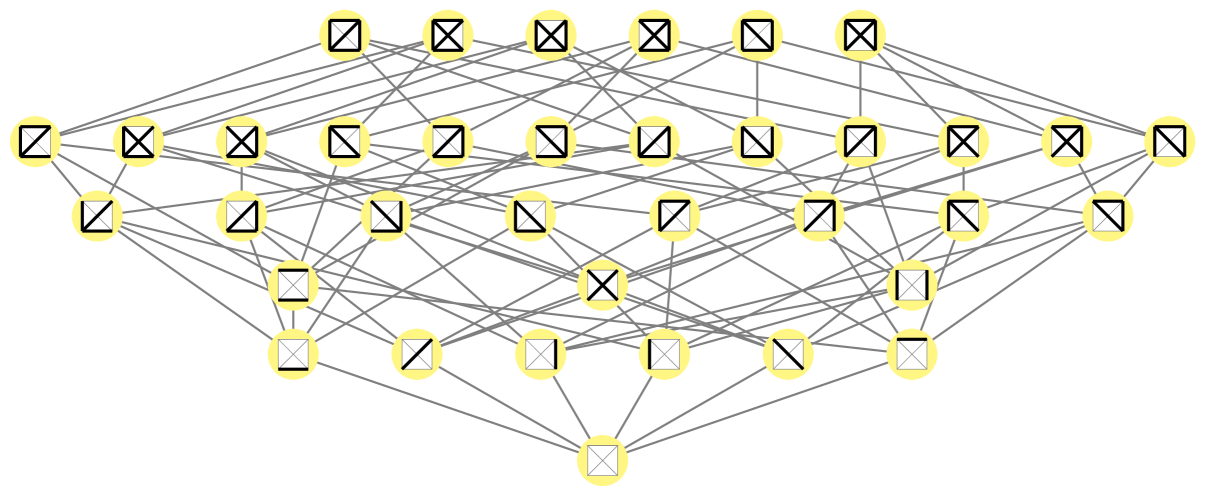
Generator belonging to an ideal is depicted as segment – in

The structure of the set of (homogeneous) prime ideals of is depicted in Figure 1. It consists of prime ideals of ranks , , , and , respectively (cf. [10, Def. 2.3] for the definition of the rank of a prime ideal), thus resulting in a model essentially different to the one presented in [8] by means of torifications, which had points, in correspondence with the coefficients of the counting polynomial . It is worth noting that despite arising from different constructions, both -models for have closed points, corresponding to the combinatorial interpretation of as the set of all subsets with two elements inside a set with four elements. These six points correspond to the -rational Tits points of , which reflect the naive notion of -rational points of an -scheme (cf. [10, Section 2.2]).
Like in the classical geometrical setting, the Grassmannian does admit a covering by six -models of affine -space, which correspond to the open subsets of where one of , , , , or is non-zero. However, these -models of affine -space are not the standard model , but the “-matrices” in case that one of , , or is non-zero, and the “twisted -matrices” in case that one of or is non-zero.
References
- [1] Chenghao Chu, Oliver Lorscheid, and Rekha Santhanam. Sheaves and -theory for -schemes. Adv. Math., 229(4):2239–2286, 2012.
- [2] Alain Connes and Caterina Consani. Characteristic , entropy and the absolute point. Preprint, arXiv:0911.3537v1, 2009.
- [3] Anton Deitmar. Schemes over . In Number fields and function fields—two parallel worlds, volume 239 of Progr. Math., pages 87–100. Birkhäuser Boston, Boston, MA, 2005.
- [4] Anton Deitmar. -schemes and toric varieties. Beiträge Algebra Geom., 49(2):517–525, 2008.
- [5] Kazuya Kato. Toric singularities. Amer. J. Math., 116(5):1073–1099, 1994.
- [6] Javier López Peña. -models for cluster algebras and total positivity. In preparation.
- [7] Javier López Peña and Oliver Lorscheid. Mapping -land. an overview of geometries over the field with one element. In Noncommutative geometry, arithmetic and related topics, pages 241–265. Johns Hopkins University Press, 2011.
- [8] Javier López Peña and Oliver Lorscheid. Torified varieties and their geometries over . Math. Z., 267(3-4):605–643, 2011.
- [9] Oliver Lorscheid. The geometry of blueprints. Part I: algebraic background and scheme theory. Adv. Math., 229(3):1804––1846, 2012.
- [10] Oliver Lorscheid. The geometry of blueprints. Part II: Tits-Weyl models of algebraic groups. Preprint, arXiv:1201.1324, 2012.
- [11] Grigory Mikhalkin. Tropical geometry. Unpublished notes, 2010.
- [12] Christophe Soulé. Les variétés sur le corps à un élément. Mosc. Math. J., 4(1):217–244, 312, 2004.
- [13] Koen Thas. Notes on , I. Combinatorics of -schemes and -geometry. In preparation.