Proofs of the Technical Results Justifying a Biologically Inspired Algorithm for Reactive Navigation of Nonholonomic Robots in Maze-Like Environments

Alexey S. Matveev almat1712@yahoo.com Michael C. Hoy mch.hoy@gmail.com Andrey V. Savkin a.savkin@unsw.edu.au Department of Mathematics and Mechanics, Saint Petersburg University, Universitetskii 28, Petrodvoretz, St.Petersburg, 198504, Russia School of Electrical Engineering and Telecommunications, The University of New South Wales, Sydney 2052, Australia

, ,

1 Introduction

Inspired by behaviors of animals, which are believed to use simple, local motion control rules that result in remarkable and complex intelligent behaviors [1, 2, 3], we examine the navigation strategy that is aimed at reaching a steady target in a steady arbitrarily shaped maze-like environment and is composed of the following reflex-like rules:

s.1)
At considerable distances from the obstacle,
1. (a)
  
  turn towards the target as quickly as possible;
2. (b)
  
  move directly to the target when headed to it;
s.2)
At a short distance from the obstacle,
1. (c)
  
  Follow (a,b) when leaving from the obstacle;
2. (d)
  
  When approaching it, quickly avert the collision threat by sharply turning.

Studies of target pursuit in animals, ranging from dragonflies to fish and dogs to humans, have suggested that they often use the pure pursuit guidance s.1) to catch not only a steady but also a moving target. The idea of local obstacle avoidance strategy s.2) is also inspired by biological examples such as a cockroach encountering a wall [2].

The rules s.1), s.2) demand only minor perceptual capacity. Access even to the distance to the obstacle is not needed: it suffices to determine whether it is short or not, and be aware of the sign of its time derivative. As for the target, the vehicle has to access its relative bearing angle. Moreover, it suffices that it is able only to recognize which quadrant of its relative Cartesian frame hosts the target line-of-sight.

To address the issue of nonholonomic constraints, control saturation, and under-actuation, we consider a vehicle of the Dubins car type. It is capable of moving with a constant speed along planar paths of upper limited curvature without reversing the direction and is controlled by the upper limited angular velocity. As a result, it is unable to slow down, stop, or make an abrupt turn.

By reliance on the bearing-only data about the target, the proposed approach is similar to the Pledge algorithm [4] and Angulus algorithm [5]. Unlike ours, the both assume access to the absolute direction (e.g., by a compass), and the latter employs not one but two angles in the convergence criterion. The major distinction is that they assume the vehicle to be able to trace the paths of unlimited curvature, in particular, broken curves and to move exactly along the obstacle boundary. These assumptions are violated in the context of this paper, which entails deficiency in the available proofs of the convergence of these algorithms.

The extended introduction and discussion of the proposed control law are given in the paper submitted by the authors to the IFAC journal Automatica. This text basically contains the proofs of the technical facts underlying justification of the convergence at performance of the proposed algorithm in that paper, which were not included into it due to the length limitations. To make the current text logically consistent, were reproduce the problem statement and notations.

2 Problem Setup and the Navigation Strategy

We consider a planar under-actuated nonholonomic vehicle of the Dubins car type. It travels with a constant speed $v$ without reversing direction and is controlled by the angular velocity $u$ limited by a given constant $\overline{u}$ . There also is a steady point target $\boldsymbol{\mathscr{T}}$ and a single steady obstacle $D\not\ni\boldsymbol{\mathscr{T}}$ in the plane, which is an arbitrarily shaped compact domain whose boundary $\partial D$ is Jordan piece-wise analytical curve without inner corners. Modulo smoothened approximation of such corners, this assumption is typically satisfied by all obstacles encountered in robotics, including continuous mazes. The objective is to drive the vehicle to the target with constantly respecting a given safety margin $d(t)\geq d_{\text{safe}}>0$ . Here $d(t)$ is the distance to the obstacle

d(t):=\text{\bf dist}_{D}[\boldsymbol{r}(t)],\qquad\text{\bf dist}_{D}[\boldsymbol{r}]:=\min_{\boldsymbol{r}_{\ast}\in D}\|\boldsymbol{r}_{\ast}-\boldsymbol{r}\|,

(1)

$\|\cdot\|$ is the Euclidian norm, and $\boldsymbol{r}(t)$ is the vehicle position.

This position is given by the abscissa $x$ and ordinate $y$ of the vehicle in the world frame, whereas its orientation is described by the angle $\theta$ from the abscissa axis to the robot centerline. The kinematics of the considered vehicles are classically described by the following equations:

\begin{array}[]{l}\dot{x}=v\cos\theta,\\ \dot{y}=v\sin\theta,\end{array},\quad\dot{\theta}=u\in[-\overline{u},\overline{u}],\quad\begin{array}[]{l}\boldsymbol{r}(0)=\boldsymbol{r}_{0}\not\in D\\ \theta(0)=\theta_{0}\end{array}.

(2)

Thus the minimal turning radius of the vehicle is equal to

R=v/\overline{u}.

(3)

The vehicle has access to the current distance $d(t)$ to $D$ and the sign $\text{\rm sgn}\dot{d}(t)$ of its time-rate $\dot{d}(t)$ , which are accessible only within the given sensor range: $d\leq d_{\text{range}}$ , where $d_{\text{range}}>d_{\text{safe}}$ . The vehicle also has access to the angle $\beta$ from its forward centerline ray to the target.

To specify the control strategy s.1), s.2), we introduce the threshold $d_{\text{trig}}<d_{\text{range}}$ separating the ’short’ and ’long’ distances to the obstacle. Mathematically, the examined strategy is given by the following concise formula:

\displaystyle u=\overline{u}\times\begin{cases}\text{\rm sgn}\beta\hfill\mid&\!\!\!\text{if}\;d>d_{\text{trig}}\;(\text{mode}\,\mathfrak{A})\\ \left\{\begin{array}[]{l l}\text{\rm sgn}\beta&\text{if}\;\dot{d}>0\\ -\sigma&\text{if}\;\dot{d}\leq 0\end{array}\right|&\!\!\!\text{if}\;d\leq d_{\text{trig}}\;(\text{mode}\,\mathfrak{B})\end{cases}.

(4)

Here $\sigma=\pm$ is a constant controller parameter, which gives the turn direction, and $\dot{d}\geq 0$ and $\dot{d}<0$ are equivalent to the vehicle orientation outwards and towards $D$ . The switch $\mathfrak{A}\mapsto\mathfrak{B}$ occurs when $d$ reduces to $d_{\text{trig}}$ ; the converse switch holds when $d$ increases to $d_{\text{trig}}$ . When mode $\mathfrak{B}$ is activated, $\dot{d}\leq 0$ ; if $\dot{d}=0$ , the ’turn’ submode $u:=-\sigma\overline{u}$ is set up. Since the control law (4) is discontinuous, the solution of the closed-loop system is meant in the Fillipov’s sense [6].

Remark 1.

In (4), $\beta$ accounts for not only the heading but also the sum of full turns performed by the target bearing.

In the basic version of the algorithm, the parameter $\sigma$ is fixed. To find a target hidden deeply inside the maze, a modified version can be employed: whenever $\mathfrak{A}\mapsto\mathfrak{B}$ , the parameter $\sigma$ is updated. The updated value is picked randomly and independently of the previous choices from $\{+,-\}$ , with the value $+$ being drawn with a fixed probability $p\in(0,1)$ . This version is called the randomized control law.

To state the assumptions, we introduce the Frenet frame $T(\boldsymbol{r}_{\ast}),N(\boldsymbol{r}_{\ast})$ of $\partial D$ at the point $\boldsymbol{r}_{\ast}\in\partial D$ ( $T$ is the positively oriented unit tangent vector, $N$ is the unit normal vector directed inwards $D$ , the boundary is oriented so that when traveling on $\partial D$ one has $D$ to the left), $\varkappa(\boldsymbol{r}_{\ast})$ is the signed curvature ( $\varkappa(\boldsymbol{r}_{\ast})<0$ on concavities) and $R_{\varkappa}(\boldsymbol{r}_{\ast}):=|\varkappa(\boldsymbol{r}_{\ast})|^{-1}$ . Due to the absence of inner corners, any point $\boldsymbol{r}\not\in D$ at a sufficiently small distance $\text{\bf dist}_{D}[\boldsymbol{r}]<d_{\star}$ from $D$ does not belong to the focal locus of $\partial D$ and $\text{\bf dist}_{D}[\boldsymbol{r}]$ is attained at only one point [7]. The regular margin $d_{\star}(D)>0$ of $D$ is the supremum of such $d_{\star}$ ’s. So $d_{\star}(D)=\infty$ for convex domains; for non-convex $D$ ,

d_{\star}(D)\leq R_{D}:=\inf_{\boldsymbol{r}\in\partial D:\varkappa(\boldsymbol{r})<0}R_{\kappa}(\boldsymbol{r}).

(5)

(The infimum over the empty set is set to be $+\infty$ .)

Assumption 1.

The vehicle is maneuverable enough: it is capable of full turn without violation of a safety margin $d_{\text{safe}}>R$ within the regularity margin of the maze $3R<d_{\star}(D)$ , and moreover $4R<R_{D}$ .

Assumption 2.

The sensor range gives enough space to avoid collision with $D$ after its detection: $d_{\text{range}}>3R$ .

The parameters $d_{\text{trig}}$ and $d_{\text{safe}}$ are tuned so that

3R<d_{\text{safe}}+2R<d_{\text{trig}}<d_{\star}(D),d_{\text{range}},R_{D}-R.

(6)

Such a choice is possible thanks to Assumptions 1 and 2.

3 Main Results

Theorem 1.

(i) With probability $1$ , the randomized control law drives the vehicle at the target $\boldsymbol{\mathscr{T}}$ for a finite time with always respecting the safety margin (i.e., there exists a time instant $t_{\ast}$ such that $\boldsymbol{r}(t_{\ast})=\boldsymbol{\mathscr{T}}$ and $\text{\bf dist}_{D}[\boldsymbol{r}(t)]\geq d_{\text{safe}}\;\forall t\in[0,t_{\ast}]$ ) whenever both the vehicle initial location $\boldsymbol{r}_{0}$ and the target are far enough from the obstacle and from each other:

\text{\bf dist}_{D}[\boldsymbol{r}_{0}]>d_{\text{trig}}+2R,\|\boldsymbol{r}_{0}-\boldsymbol{\mathscr{T}}\|>2R,\text{\bf dist}_{D}[\boldsymbol{\mathscr{T}}]>d_{\text{trig}}.

(7)

(ii) The basic control law drives the vehicle at the target for a finite time with always respecting the safety margin whenever (7) holds and the vehicle initial location and the target lie far enough from the convex hull $\text{\bf co}\;D$ of the maze: $\text{\bf dist}_{\text{\bf co}\;D}[\boldsymbol{\mathscr{T}}]>d_{\text{trig}},\text{\bf dist}_{\text{\bf co}\;D}[\boldsymbol{r}_{0}]>d_{\text{trig}}$ .

In (7), $\text{\bf dist}_{D}[\boldsymbol{r}_{0}]>d_{\text{trig}}+2R$ can be relaxed into $\text{\bf dist}_{D}[\boldsymbol{r}_{0}]>d_{\text{trig}}$ if the vehicle is initially directed to the target $\beta(0)=0$ . In view of (3) and the freedom (6) in the choice of $d_{\text{safe}},d_{\text{trig}}$ , not only Assumptions 1, 2 but also the constraints (7) disappear (are boiled down into $\text{\bf dist}_{D}[\boldsymbol{r}_{0}]>0,\|\boldsymbol{r}_{0}-\boldsymbol{\mathscr{T}}\|>0,\text{\bf dist}_{D}[\boldsymbol{\mathscr{T}}]>0$ ) as $v\to 0$ . In other words, the algorithm succeeds in any case if the cruise speed $v$ is small enough.

The last assumption $\text{\bf dist}_{\text{\bf co}\;D}[\boldsymbol{\mathscr{T}}]>d_{\text{trig}}$ from (ii) can be relaxed to cover some scenarios with the target inside the maze. To specify this, we need some notations and definitions.

The $d$ -equidistant curve $C(d)$ of $D$ is the locus of points $\boldsymbol{r}$ at the distance $\text{\bf dist}_{D}[\boldsymbol{r}]=d$ from $D$ ; the $d$ -neighborhood $N(d)$ of $D$ is the area bounded by $C(d)$ ; $[\boldsymbol{r}_{1},\boldsymbol{r}_{2}]$ is the straight line segment directed from $\boldsymbol{r}_{1}$ to $\boldsymbol{r}_{2}$ .

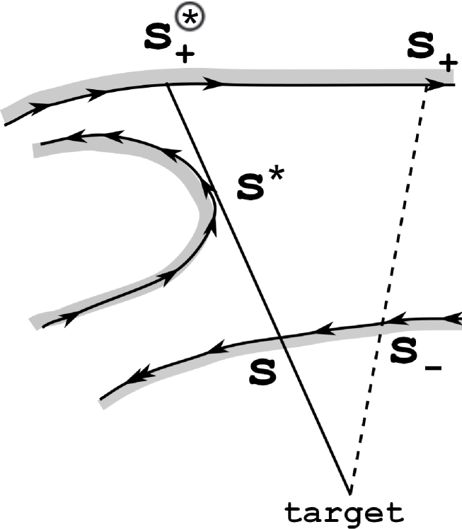
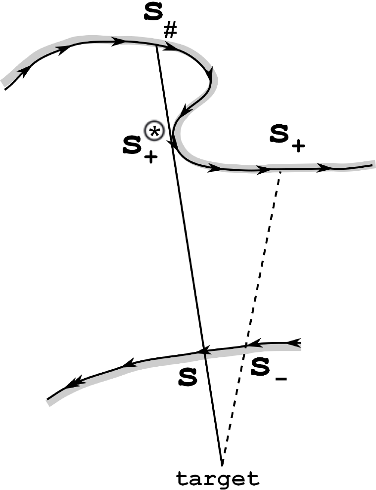
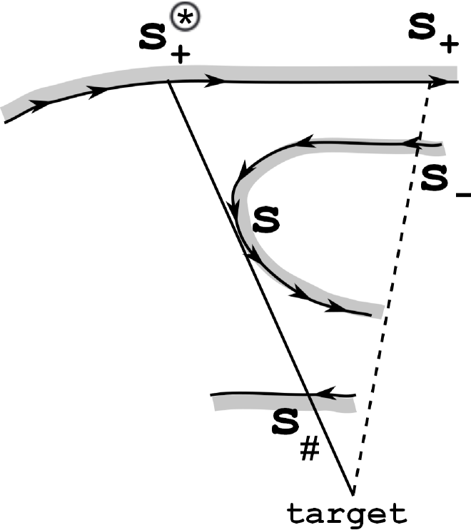
Let $\boldsymbol{r}_{\lozenge},\boldsymbol{r}_{\ast}\in C(d_{\text{trig}})$ and $(\boldsymbol{r}_{\lozenge},\boldsymbol{r}_{\ast})\cap N(d_{\text{trig}})=\emptyset$ . The points $\boldsymbol{r}_{\lozenge},\boldsymbol{r}_{\ast}$ divide $C(d_{\text{trig}})$ into two arcs. Being concatenated with $[\boldsymbol{r}_{\lozenge},\boldsymbol{r}_{\ast}]$ , each of them gives rise to a Jordan curve encircling a bounded domain, one of which is the other united with $N(d_{\text{trig}})$ . The smaller domain is called the simple cave of $N(d_{\text{trig}})$ with endpoints $\boldsymbol{r}_{\lozenge},\boldsymbol{r}_{\ast}$ . The location $\boldsymbol{r}$ is said to be locked if it belongs to a simple cave of $N(d_{\text{trig}})$ whose endpoints lie on a common ray centered at $\boldsymbol{\mathscr{T}}$ . We remark that if $\text{\bf dist}_{\text{\bf co}\;D}[\boldsymbol{r}]>d_{\text{trig}}$ , the location is unlocked.

Theorem 2.

The basic control law drives the vehicle at the target for a finite time with always respecting the safety margin whenever (7) holds and both the initial location of the vehicle and the target are unlocked.

Now we disclose the tactical behavior implied by s.1), s.2) and show that it includes wall following in a sliding mode. In doing so, we focus on a particular avoidance maneuver (AM), i.e., the motion within uninterrupted mode $\mathfrak{B}$ .

Let $\boldsymbol{\rho}(s)$ be the natural parametric representation of $\partial D$ , where $s$ is the curvilinear abscissa. This abscissa is cyclic: $s$ and $s+L$ encode a common point, where $L$ is the perimeter of $\partial D$ . We notationally identify $s$ and $\boldsymbol{\rho}(s)$ . For any $\boldsymbol{r}\not\in D$ within the regular margin $\text{\bf dist}_{D}[\boldsymbol{r}]<d_{\star}(D)$ , the symbol $s(\boldsymbol{r})$ stands for the boundary point closest to $\boldsymbol{r}$ , and $s(t):=s[\boldsymbol{r}(t)]$ , where $\boldsymbol{r}(t)$ is the vehicle location at time $t$ .

To simplify the matters, we first show that $\partial D$ can be assumed $C^{1}$ -smooth without any loss of generality. Indeed, if $0<d<d_{\star}(D)$ , the equidistant curve $C(d)$ is $C^{1}$ -smooth and piece-wise $C^{2}$ -smooth [7]; its parametric representation, orientation, and curvature are given by

s\mapsto\boldsymbol{\rho}(s)-dN(s),\qquad\varkappa_{C(d)}(s)=\frac{\varkappa(s)}{1+\varkappa(s)d}.

(8)

The second formula holds if $s$ is not a corner point of $\partial D$ ; such points contribute circular arcs of the radius $d$ into $C(d)$ . So by picking $\delta>0$ small enough, expanding $D$ to $N(\delta)$ , and correction $\mathfrak{d}:=\mathfrak{d}-\delta$ of $\mathfrak{d}:=d,d_{\text{safe}},d_{\text{trig}},d_{\text{range}}$ , we keep all assumptions true and do not alter the operation of the closed-loop system. Hence $\partial D$ can be assumed $C^{1}$ -smooth.

Writing $f(\eta_{\ast}\pm^{\text{\tiny$\approx$}}\!0)>0$ means that there exists small enough $\Delta>0$ such that $f(\eta)>0$ if $0<\pm(\eta-\eta_{\ast})<\Delta$ . The similar notations, e.g., $f(\eta_{\ast}\pm^{\text{\tiny$\approx$}}\!0)\leq 0$ , are defined likewise.

Proposition 3.

Let for the vehicle driven by the control law (4), obstacle avoidance be started with zero target bearing $\beta(t)=0$ at $t=t_{\ast}$ . Then the following claims hold:

(i)

There exists $\tau\geq t_{\ast}$ such that the vehicle moves with the maximal steering angle $u\equiv-\sigma\overline{u}$ and the distance to the obstacle decreases $\dot{d}\leq 0$ until $\tau$ ,^*^**This part of AM is called the initial turn and abbreviated IT. and at $t=\tau$ , the sliding motion along the equidistant curve $C\left\{\text{\bf dist}_{D}[\boldsymbol{r}(\tau)]\right\}$ ^†^††This is abbreviated SMEC and means following the wall at the fixed distance $\text{\bf dist}_{D}[\boldsymbol{r}(\tau)]$ , which is set up at the start of SMEC. is started with $\sigma\dot{s}>0$ and $\beta\dot{s}>0$ ;
(ii)

SMEC holds until $\beta$ arrives at zero at a time when $\varkappa[s(t)+\sigma^{\text{\tiny$\approx$}}\!0]>0$ , which sooner or later holds and after which a straight move to the target^‡^‡‡SMT, which is sliding motion over the surface $\beta=0$ is commenced;
(iii)

During SMT, the vehicle first does not approach the obstacle $\dot{d}\geq 0$ and either the triggering threshold $d_{\text{trig}}$ is ultimately trespassed and so mode $\mathfrak{B}$ is switched off, or a situation is encountered where $\dot{d}(t)=0$ and $\varkappa[s(t)+\sigma^{\text{\tiny$\approx$}}\!0]<0$ . When it is encountered, the vehicle starts SMEC related to the current distance;
(iv)

There may be several transitions from SMEC to SMT and vice versa, all obeying the rules from (ii), (iii);
(v)

The number of transitions is finite and finally the vehicle does trespass the triggering threshold $d_{\text{trig}}$ , thus terminating the considered avoidance maneuver;
(vi)

Except for the initial turn described in (i), the vehicle maintains a definite direction of bypassing the obstacle: $\dot{s}$ is constantly positive if $\sigma=+$ (counterclockwise bypass) and negative if $\sigma=-$ (clockwise bypass).

By (4), AM is commenced with $\dot{d}(t_{\ast})\leq 0$ . The next remark shows that if $\dot{d}(t_{\ast})=0$ , IT may have the zero duration.

Remark 3.1.

If $\dot{d}(t_{\ast})=0$ , IT has the zero duration if and only if $\sigma\dot{s}(t_{\ast})>0$ . Then the following claims are true:

1.

If $\varkappa[s(t_{\ast})+\sigma\cdot^{\text{\tiny$\approx$}}\!0]<0$ , SMEC is immediately started;
2.

If $\varkappa[s(t_{\ast})+\sigma\cdot^{\text{\tiny$\approx$}}\!0]\geq 0$ , the duration of SMEC is zero, and SMT is continued.

The assumption $\beta(t_{\ast})=0$ of Proposition 3 holds for the first AM due to (7). Indeed, since $\text{\bf dist}_{D}[\boldsymbol{r}_{0}]>d_{\text{trig}}+2R$ , the pursuit guidance law turns the vehicle towards the target earlier than the threshold $d_{\text{trig}}$ for activation of AM is encountered. It also holds for all subsequent AM’s since any AM ends in course of SMT by Proposition 3.

4 Technical facts underlying the proofs of Proposition 3 and Remark 3.1.

4.1 Geometrical Preliminaries

We assume that the world frame (WF) is centered at the target $\boldsymbol{\mathscr{T}}$ . Let $C\not\ni\boldsymbol{\mathscr{T}}$ be a regular piece-wise smooth directed curve with natural parametric representation $\boldsymbol{\varrho}(s),s\in[s_{-},s_{+}]$ . The turning angle of $C$ around a point $\boldsymbol{p}\not\in C$ is denoted by $\sphericalangle_{\boldsymbol{p}}C$ , and $\sphericalangle\text{\bf TANG}\left[C\right]:=\sphericalangle_{0}T$ , where $T(s),N(s)$ is the Frenet frame of $C$ at $s$ .^§^§§ At the corner points, the count of $\sphericalangle_{0}T$ progresses abruptly according to the conventional rules [7]. Let $\lambda(s),\zeta(s)$ and $\psi(s)$ stand for the Cartesian coordinates and polar angle of $-\boldsymbol{\varrho}(s)$ in this frame (see Fig.1(a)), respectively,

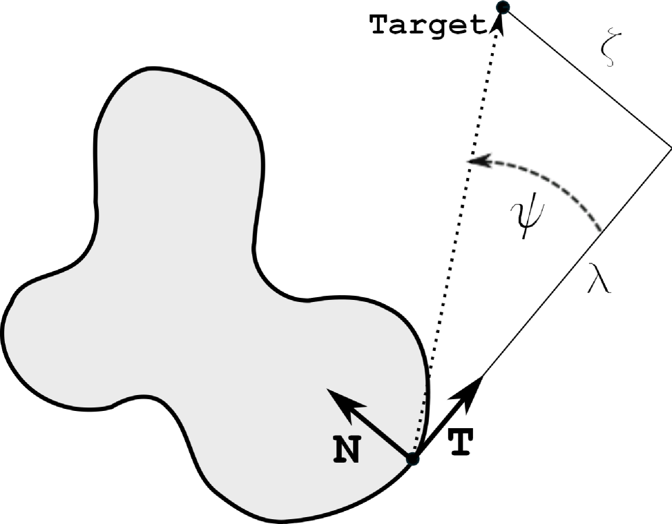
Refer to caption — Figure 1: (a) Definition of $\lambda$ and $\zeta$ ; (b) Behavior during IT.

and let ^′ denote differentiation with respect to $s$ . The polar angle of $\boldsymbol{\varrho}(s)$ in WF and the curvature of $C$ at $s$ are denoted by $\varphi(s)$ and $\varkappa(s)$ , respectively. To indicate the curve $C$ , the symbols $T,N,\lambda,\zeta,\varkappa$ , etc. may be supplied with the lower index _C. The directed curve traced as $s$ runs from $s_{1}$ to $s_{2}$ is denoted by $C_{s_{1}\xrightarrow{\pm}s_{2}}$ , where the specifier $\pm$ is used for closed curves. The superscript ^a means that the lemma is equipped with the number under which its formulation is given in the basic version of the paper.

Lemma 4.

^a The following relations hold whenever $\boldsymbol{\mathscr{T}}\not\in C$ :

	$\displaystyle\begin{array}[]{l}\lambda^{\prime}=-1+\varkappa\zeta\\ \zeta^{\prime}=-\varkappa\lambda\end{array},\quad\begin{array}[]{r}\psi^{\prime}=-\varkappa+\zeta(\lambda^{2}+\zeta^{2})^{-1}\\ \varphi^{\prime}=\zeta(\lambda^{2}+\zeta^{2})^{-1}\end{array},$		(13)
	$\displaystyle\text{\large$\mathfrak{r}$}:=\,\mbox{\bf col}\,(\lambda,\zeta)\neq 0,\sphericalangle_{0}\text{\large$\mathfrak{r}$}=\sphericalangle_{\boldsymbol{\mathscr{T}}}C-\sphericalangle\text{\bf TANG}\left[C\right].$		(14)

\pf

Differentiation of the equation $\boldsymbol{\mathscr{T}}=\boldsymbol{\varrho}+\lambda T+\zeta N$ and the Frenet-Serret formulas $T^{\prime}=\kappa N,N^{\prime}=-\kappa T$ [7] yield that $0=T+\lambda^{\prime}T+\lambda\varkappa N+\zeta^{\prime}N-\zeta\varkappa T.$ Equating the cumulative coefficients in this linear combination of $T$ and $N$ to zero gives the first two equations in (13). By virtue of them, the third and forth ones follow from [7]

\psi^{\prime}=\frac{\zeta^{\prime}\lambda-\lambda^{\prime}\zeta}{\lambda^{2}+\zeta^{2}},\qquad\varphi^{\prime}=\frac{y^{\prime}x-x^{\prime}y}{x^{2}+y^{2}}.

(15)

The first relation in (14) holds since $\boldsymbol{\mathscr{T}}\not\in C$ . Let $\eta(s):=\sphericalangle\text{\bf TANG}\big{[}T_{s_{-}\to s-0}\big{]}+\eta_{0}$ , where $\eta_{0}$ is the polar angle of $T(s_{-})$ . The matrix $\Phi_{\eta(s)}$ of rotation through $\eta(s)$ transforms the world frame into the Frenet one, and $\boldsymbol{\varrho}(s)=h(s)\,\mbox{\bf col}\,[\cos\varphi(s),\sin\varphi(s)]$ . So $\text{\large$\mathfrak{r}$}(s)=-\Phi_{-\eta(s)}\boldsymbol{\varrho}(s)=h(s)\,\mbox{\bf col}\,\{[\cos[\pi+\varphi(s)-\eta(s)],\sin[\pi+\varphi(s)-\eta(s)]\}$ . Thus $\pi+\varphi(s)-\eta(s)$ is the piece-wise continuous polar angle of $\text{\large$\mathfrak{r}$}(s)$ that jumps according to the convention concerned by footnote ${}^{\text{\ref{foot.conv}}}$ . This trivially implies (14). $\quad\bullet$

Corollary 4.1.

Let $\zeta(s_{\ast})=0$ and $\varsigma=\pm$ . Then

\begin{array}[]{r c l}\varsigma\zeta[s_{\ast}+\varsigma^{\text{\tiny$\approx$}}\!0]\text{\rm sgn}\lambda[s_{\ast}]<0&\text{\rm if}&\varkappa[s_{\ast}+\varsigma^{\text{\tiny$\approx$}}\!0]>0\\ \varsigma\zeta[s_{\ast}+\varsigma^{\text{\tiny$\approx$}}\!0]\text{\rm sgn}\lambda[s_{\ast}]>0&\text{\rm if}&\varkappa[s_{\ast}+\varsigma^{\text{\tiny$\approx$}}\!0]<0\end{array}.

(16)

By (6) and the last inequality in (7), Lemma LABEL:lem.geom yields

\sphericalangle_{0}\text{\large$\mathfrak{r}$}_{C(d_{\ast})}=-2\pi\qquad\text{for}\quad d_{\ast}\in[0,d_{\text{trig}}].

(17)

Corollary 4.2.

There exist $F$ and $d_{\#}>d_{\text{trig}}$ such that whenever $|d|\leq d_{\#}$ , the set $S(d):=\{s\in\partial D:\zeta_{\partial D}(s)=d\}$ has no more than $F$ connected components.

\pf

By the last inequality in (7), $\exists d_{\#}:d_{\text{trig}}<d_{\#}<\text{\bf dist}_{D}[\boldsymbol{\mathscr{T}}]\leq\sqrt{\zeta(s)^{2}+\lambda(s)^{2}}$ . Then $s\in S(d)\wedge|d|\leq d_{\#}\Rightarrow|\lambda(s)|\geq\delta:=\sqrt{\text{\bf dist}_{D}[\boldsymbol{\mathscr{T}}]^{2}-d_{\#}^{2}}>0$ . Since the domain $D$ is compact, $|\lambda^{\prime}(s)|\leq M<\infty\;\forall s$ . So whenever $s\in S(d)$ and $|d|\leq d_{\#}$ , the function $\lambda(\cdot)$ does not change its sign in the $\delta M^{-1}$ -neighborhood $V(s)$ of $s$ .

Since $\partial D$ is piece-wise analytical, each set $\{s:\pm\varkappa(s)>0\}$ and $\{s:\varkappa(s)=0\}$ has finitely many connected components $\partial^{\pm}_{i}$ and $\partial^{0}_{\nu}$ , respectively. By the foregoing and (13), any intersection $V(s)\cap\overline{\partial^{\pm}_{i}},s\in S(d),|d|\leq d_{\#}$ contains only one point $s$ . Hence the entire arc $\partial^{\pm}_{i}$ of the length $\left|\partial^{\pm}_{i}\right|$ contains no more than $\delta^{-1}M\left|\partial^{\pm}_{i}\right|+1$ such points. It remains to note that $S(d)$ covers any $\partial^{0}_{\nu}$ such that $\partial^{0}_{\nu}\cap S(d)\neq\emptyset$ . $\quad\bullet$

Observation 1.

SMEC with $\sigma=\pm$ ends when $s\in S_{0}:=\{s\in\partial D:-d_{\#}<\zeta_{\partial D}(s)<0,\pm\lambda_{\partial D}(s)>0\}$ . This set has no more than $F$ connected components, called $\pm$ arcs.

The second claim holds since $\lambda^{\prime}<0$ on $S_{0}$ due to (6), (13).

4.2 Technical Facts

Lemma 5.

The following two statements hold:
(i) In the domain $d\leq d_{\text{trig}}\wedge\dot{d}>0\vee d>d_{\text{trig}}$ , the surface $\beta=0$ is sliding, with the equivalent control [6] $u\equiv 0$ ;
(ii) The surface $\dot{d}=0$ is sliding in the domain

d_{\text{trig}}-2R\leq d<d_{\text{trig}},\quad\dot{s}\beta>0,\quad\sigma\dot{s}>0.

(18)

\pf

(i) Let $h$ be the distance from the vehicle to $\boldsymbol{\mathscr{T}}$ . Due to (2), $\dot{h}=-v\cos\beta,\dot{\beta}=h^{-1}v\sin\beta-u$ . So as the state approaches the surface $\beta=0$ , we have $\dot{\beta}\overset{\eqref{c.a}}{\to}-\overline{u}\text{\rm sgn}\beta$ , which implies the first claim.

(ii) Let $\alpha$ be the polar angle of the vehicle velocity in the frame $T_{\partial D}[s(t)],N_{\partial D}[s(t)]$ . By (5), (6), and (18), $1+\varkappa[s(t)]d(t)>0$ , and as is shown in e.g., [8],

\dot{s}=\frac{v\cos\alpha}{1+\varkappa(s)d},\;\dot{d}=-v\sin\alpha,\;\dot{\alpha}=-\varkappa(s)\dot{s}+u.

(19)

As the state approaches a point where $\dot{d}=0$ and (18) holds,

\begin{array}[]{l}\sin\alpha\to 0\\ \cos\alpha\to\text{\rm sgn}\dot{s}\end{array},\ddot{d}\to-v^{2}\left[\frac{u}{v}\text{\rm sgn}\dot{s}-\frac{\varkappa}{1+\varkappa d}\right].

(20)

If the state remains at a definite side of the surface $\dot{d}=0$ , (3) and (4) yield that

	$\displaystyle\ddot{d}\xrightarrow{\dot{d}>0}\ddot{d}_{+}:=-v^{2}\left[\frac{1}{R}\text{\rm sgn}(\beta\dot{s})-\frac{\varkappa}{1+\varkappa d}\right]$
	$\displaystyle\overset{\text{\eqref{sub-dom}}}{=}-v^{2}\left[\frac{1}{R}-\frac{\varkappa}{1+\varkappa d}\right],\qquad\ddot{d}\xrightarrow{\dot{d}<0}\ddot{d}_{-}:=$
	$\displaystyle v^{2}\left[\sigma\frac{1}{R}\text{\rm sgn}\dot{s}+\frac{\varkappa}{1+\varkappa d}\right]\overset{\text{\eqref{sub-dom}}}{=}v^{2}\left[\frac{1}{R}+\frac{\varkappa}{1+\varkappa d}\right].$		(21)

The proof is completed by observing that by (6), (18),

	$\displaystyle\ddot{d}_{+}=-v^{2}\frac{1+\varkappa d-\varkappa R}{R(1+\varkappa d)}<0\text{since}\begin{array}[]{l}1+\varkappa d>0\;\text{and}\\ d>d_{\text{safe}}>R\end{array}$		(24)
	$\displaystyle\ddot{d}_{-}=v^{2}\frac{\|\varkappa\|\left[R_{\varkappa}+(d+R)\text{\rm sgn}\varkappa\right]}{R(1+\varkappa d)}>0.$		(25)

The subsequent proofs are focused on $\sigma=+$ ; the case $\sigma=-$ is considered likewise.

Lemma 6.

If $\dot{d}(t_{\ast})<0$ , claim (i) in Proposition 3 is true.

\pf

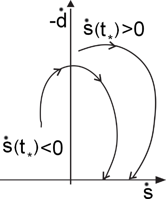
Let $\sigma=+$ . Due to (4), initially $u\equiv-\overline{u}$ . Let $[t_{\ast},\tau]$ denote the maximal interval on which $u\equiv-\overline{u}$ . For $t\in(t_{\ast},\tau)$ , the vehicle moves clockwise along a circle $C_{\text{in}}$ of the radius $R$ and so by Remark 1, $\beta(t)>0$ and

d(t)\geq\text{\bf dist}_{D}[\boldsymbol{r}(0)]-\underbrace{\|\boldsymbol{r}-\boldsymbol{r}(0)\|}_{\leq 2R}\\ \geq d_{\text{trig}}-2R\overset{\text{\eqref{eq.trig}}}{>}d_{\text{safe}}>R>0.

(26)

\dot{\alpha}\overset{\text{\eqref{eq1}}}{=}-v\left[\frac{\varkappa\cos\alpha}{1+\varkappa d}+\frac{\overline{u}}{v}\right]\\ \overset{\text{\eqref{Rmin}}}{\leq}-v\left[\frac{1}{R}-\frac{|\varkappa|}{1+\varkappa d}\right]=-v\left[\frac{1}{R}-\frac{1}{R_{\varkappa}+d\text{\rm sgn}\varkappa}\right].

While $d\leq d_{\text{trig}}$ (in particular, while $\dot{d}\leq 0$ ) the expression in the last square brackets is positive. This is true by (26) if $\varkappa\geq 0$ ; otherwise, since $R_{\varkappa}>R+d_{\text{trig}}$ by (6). So $\dot{\alpha}\leq-\delta<0$ , i.e., the vector $\,\mbox{\bf col}\,(\cos\alpha,\sin\alpha)$ rotates clockwise. Here the signs of the first and second components equal those of $\dot{s}$ and $-\dot{d}$ , respectively, by (19) and so $\,\mbox{\bf col}\,(\dot{s},\dot{d})$ evolves as is illustrated in Fig. 1(b). This and the conditions (18) for the sliding motion complete the proof. $\quad\bullet$

More can be derived from the above proof.

Lemma 9.

^a Let $s_{\ast}$ and $s_{b}$ be the values of the continuously evolving $s$ at the start and end of IT, respectively. During IT, $\sigma\dot{s}\geq 0$ if $\sigma\dot{s}(t_{\ast})\geq 0$ , and $\dot{s}$ ones changes the sign otherwise. In any case, $s$ runs from $s_{\ast}$ to $s_{b}$ in the direction $\sigma$ during a last phase of IT.

\pf

Let $\sigma=+$ . The map $\boldsymbol{r}\mapsto(s,d)$ is the orientation-reversing immersion on the disc $D_{\text{in}}$ encircled by $C_{\text{in}}$ . So it transforms any negatively oriented circle $C\subset D_{\text{in}}$ concentric with $C_{\text{in}}$ into a curve $\xi$ with $\sphericalangle\text{\bf TANG}\left[\xi\right]=2\pi$ . Then the argument from the concluding part of the proof of Lemma 6 shows that as the robot once runs over $C_{\text{in}}$ in the negative direction, the vector $\,\mbox{\bf col}\,(\dot{s},\dot{d})$ intersects the half-axes of the frame in the order associated with counter clockwise rotation, each only once. This immediately implies the claim given by the first sentence in the conclusion of the lemma.

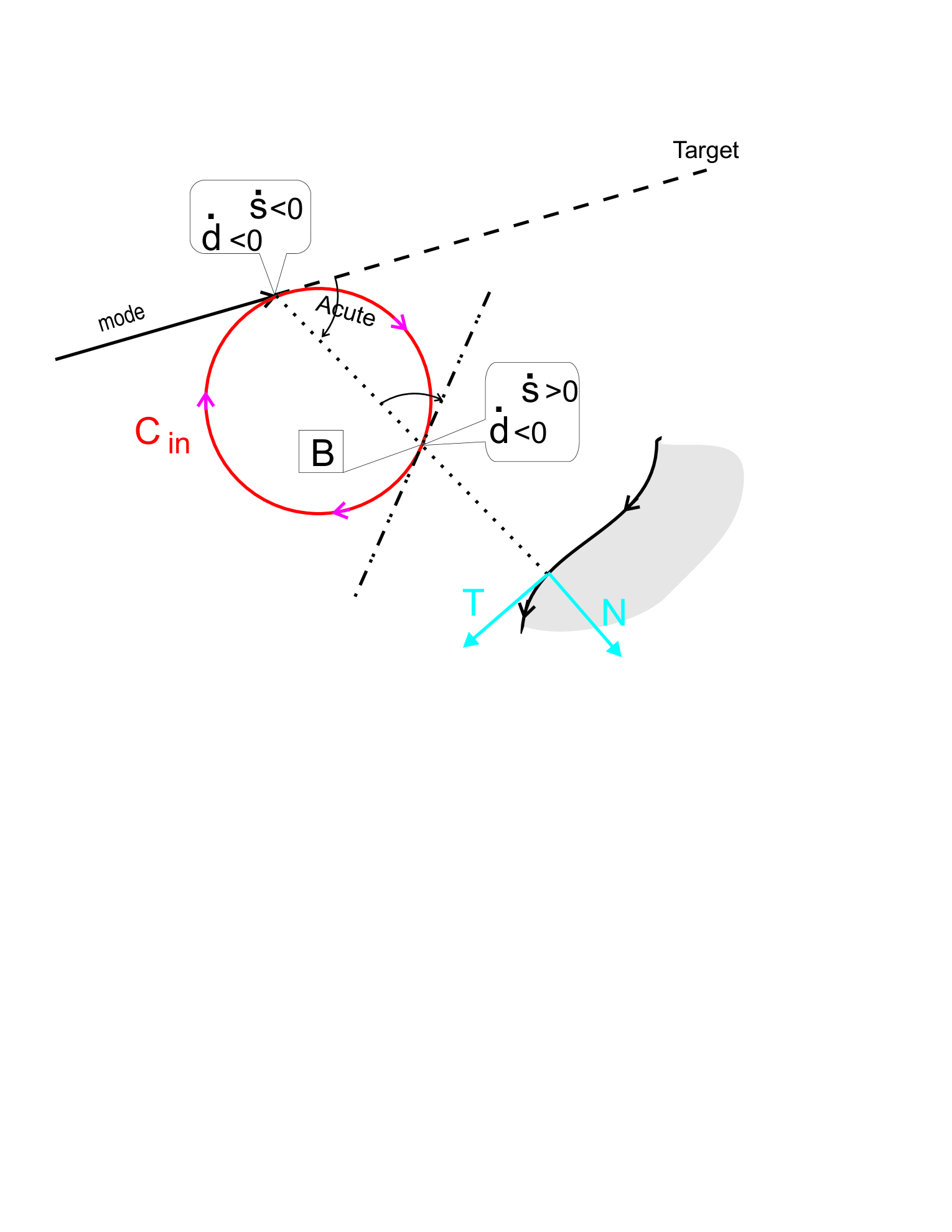
If $\dot{s}(t_{\ast})\geq 0$ , this claim yields that $s_{b}-s_{\ast}\geq 0$ . Let $\dot{s}(t_{\ast})<0$ . As the robot once runs over $C_{\text{in}}$ in the negative direction, $\dot{s}>0$ and $\dot{d}\leq 0$ when it passes the point $B$ from Fig. 2(a), which corresponds to the second passage of $s=s_{\ast}$ . Due to the order in which $\,\mbox{\bf col}\,(\dot{s},\dot{d})$ intersects the half-axes, this combination of signs is possible only before $\dot{d}$ vanishes for the first time, i.e., within IT. Thus the second occurrence of $s=s_{\ast}$ holds within IT. The proof is completed by noting that $\dot{s}>0$ after this by the first claim of the lemma. $\quad\bullet$

We proceed to the case where some of the vector fields is tangential to the discontinuity surface $\dot{d}=0$ . Since this may undermine uniqueness of the solution (its existence is still guaranteed), the arguments become much more sophisticated. The first lemma establishes a required technical fact. To state it, we note that whenever $d:=\text{\bf dist}_{D}[\boldsymbol{r}]<R_{\star}(D)$ , the system state $(x,y,\theta)$ is given by $s,d,\theta$ and along with $(\dot{d},\dot{s})\neq(0,0)$ , uniquely determines $\beta\in(-\pi,\pi)$ .

Lemma 7.

If $\lambda_{C(d_{\dagger})}(s_{\ast})\neq 0$ for $d_{\dagger}\in[0,d_{\text{trig}}]$ , there exists $\delta>0$ such that whenever $s_{\ast}\leq s_{0}<s<s_{\ast}+\delta$ and $|d_{\ast}-d_{\dagger}|<\delta$ , the following entailments hold with $\varsigma:=\text{\rm sgn}\dot{s}$ :

	$\displaystyle\begin{array}[]{c}\dot{s}\neq 0,\dot{d}\geq 0,d\geq d_{\ast},\zeta_{C(d_{\ast})}(s_{0})\geq 0\\ \varkappa(s_{\ast}+\varsigma^{\text{\tiny$\approx$}}\!0)<0,\dot{s}\lambda_{C(d_{\dagger})}(s_{0})>0\end{array}\Rightarrow\dot{s}\beta>0;$		(29)
	$\displaystyle\begin{array}[]{c}\dot{s}\neq 0,\dot{d}\leq 0,d\leq d_{\ast},\zeta_{C(d_{\ast})}(s_{0})\leq 0\\ \varkappa(s_{\ast}+\varsigma^{\text{\tiny$\approx$}}\!0)\geq 0,\dot{s}\lambda_{C(d_{\dagger})}(s_{0})>0\end{array}\Rightarrow\dot{s}\beta\leq 0.$		(32)

In (32), $\dot{s}\beta<0$ if $\zeta_{C(d_{\ast})}(s_{0})<0$ or $\varkappa\not\equiv 0$ on $\partial D_{s_{0}\to s}$ .

\pf

We pick $\delta>0$ so that $\lambda_{C(d_{\ast})}(s)$ and $\varkappa(s)$ do not change the sign as $s$ and $d_{\ast}$ run over $(s_{\ast},s_{\ast}+\delta)$ and $(d_{\dagger}-\delta,d_{\dagger}+\delta)$ , respectively. By (8), the curvature $\varkappa_{C(d_{\ast})}(s)$ does not change its sign either, which equals $\text{\rm sgn}\varkappa(s_{\ast}+\varsigma^{\text{\tiny$\approx$}}\!0)$ .

If the conditions from (29) hold and $\varsigma=+$ , application of the second equation from (13) to $C(d_{\ast})$ yields that $\zeta_{C(d_{\ast})}(s)>0$ . So the target polar angle in the $s$ -related Frenet frame of $C(d_{\ast})$ belongs to $(0,\pi/2)$ . Transformation of this frame into that of the vehicle path consists in a move of the origin in the negative direction along the $\zeta$ -axis (since $d\geq d_{\ast}$ ) and a clockwise rotation of the axes (since $\dot{d}>0,\dot{s}>0$ ). Since both operations increase the target bearing angle, $\beta>0$ . Formula (29) with $\varsigma=-$ and (32) are established likewise. $\quad\bullet$

Lemma 7.

^a Let $d_{\text{safe}}\leq d_{\ast}:=d(t_{\ast})\leq d_{\text{trig}}$ , $\dot{d}(t_{\ast})=0$ at a time $t_{\ast}$ within mode $\mathfrak{B}$ . Then for $t>t_{\ast},t\approx t_{\ast}$ , the robot

i)

performs the turn with $u\equiv-\sigma\overline{u}$ if $\sigma\dot{s}(t_{\ast})<0$ , $d(t_{\ast})=d_{\text{trig}}$ , and $\beta(t_{\ast})=0$ ;
ii)

undergoes SMEC if $\sigma\dot{s}(t_{\ast})>0$ and either (1) $\sigma\beta(t_{\ast})>0$ or (2) $\beta(t_{\ast})=0$ and $\varkappa[s(t_{\ast})+\text{\rm sgn}\dot{s}(t_{\ast})^{\text{\tiny$\approx$}}\!0]<0$ ;
iii)

moves straight to the target if $\beta(t_{\ast})=0,\sigma\dot{s}(t_{\ast})>0,\varkappa[s(t_{\ast})+\text{\rm sgn}\dot{s}(t_{\ast})^{\text{\tiny$\approx$}}\!0]\geq 0$ .

\pf

Let $\sigma=+$ . i) As $t\to t_{\ast}$ , (4) and (20) yield that

\ddot{d}|_{u=-\overline{u}}\to v^{2}\left[-\frac{1}{R}+\frac{\varkappa}{1+\varkappa d_{\ast}}\right]=-\frac{1+\varkappa[d_{\ast}-R]]}{R(1+\varkappa d_{\ast})}<0,

(33)

where $\varkappa:=\varkappa[s(t_{\ast})\pm 0]$ and the inequality holds since $d_{\ast}\geq d_{\text{safe}}>R$ due to (6).

Let i) fail to be true and $\varkappa[s(t_{\ast})-^{\text{\tiny$\approx$}}\!0]<0$ . If there exists an infinite sequence $\{t_{i}\}$ such that $t_{i}>t_{\ast},d(t_{i})<d_{\text{trig}}\;\forall i$ and $t_{i}\to t_{\ast}$ as $i\to\infty$ , a proper decrease of every $t_{i}$ yields in addition that $\dot{d}(t_{i})<0$ since $d(t_{\ast})=d_{\text{trig}}$ . However then $\dot{d}(t)<0$ for $t\geq t_{i},t\approx t_{\ast}$ by (4), (33) and thus $\dot{d}(t)<0,d(t)<d_{\text{trig}}$ for $t>t_{\ast},t\approx t_{\ast}$ , i.e., (i) holds in violation of the initial assumption. It follows that $d(t_{\ast}+^{\text{\tiny$\approx$}}\!0)\geq d_{\text{trig}}$ .

Now suppose that there is a sequence $\{t_{i}\}$ such that $t_{i}>t_{\ast},d(t_{i})=d_{\text{trig}}\;\forall i$ , $t_{i}\to t_{\ast}$ as $i\to\infty$ . Then $\dot{d}(t_{i})=0$ and so $\beta(t_{i})<0$ due to (29). By continuity, $\beta<0$ in a vicinity of the system state at $t=t_{i}$ . Then any option from (4) yields $u=-\overline{u}$ and so $u(t)\equiv-\overline{u}\;\forall t\approx t_{i}$ by the definition of Filippov’s solution. Hence $d(t_{i})=d_{\text{trig}}\wedge\dot{d}(t_{i})=0\overset{\text{\eqref{u.minus}}}{\Rightarrow}d(t_{i}+^{\text{\tiny$\approx$}}\!0)<d_{\text{trig}}$ , in violation of the foregoing. So $d>d_{\text{trig}}$ and $u=\text{\rm sgn}\beta$ for $t>t_{\ast},t\approx t_{\ast}$ by (4), and by Lemma 5, SMT is continued. Then the last relation in (20) (with $u:=0$ ) and $\varkappa[s(t_{\ast})-^{\text{\tiny$\approx$}}\!0]<0$ imply the contradiction $d(t_{\ast}+^{\text{\tiny$\approx$}}\!0)<d_{\text{trig}}$ to the foregoing, which proves i).

Let $\varkappa[s(t_{\ast})-^{\text{\tiny$\approx$}}\!0]\geq 0$ . So far as the controller is first probationally set to the submode related with $\dot{d}<0$ , this submode will be maintained longer by (33).

ii.1) If $d(t_{\ast})<d_{\text{trig}}$ , the claim is true by Lemma 5. Let $d(t_{\ast})=d_{\text{trig}}$ . If there is a sequence $\{t_{i}\}$ such that $t_{i}>t_{\ast},d(t_{i})<d_{\text{trig}}\;\forall i$ and $t_{i}\to t_{\ast}$ as $i\to\infty$ , a proper decrease of every $t_{i}$ yields in addition that $\dot{d}(t_{i})<0$ . Let $\tau_{i}$ be the minimal $\tau\in[t_{\ast},t_{i}]$ such that $d(t)<d_{\text{trig}}$ and $\dot{d}(t)<0$ for $t\in(\tau,t_{i}]$ . For such $t$ , $u\equiv-\overline{u}$ by (4) and so $\ddot{d}>0$ by (21) and (25). So $\dot{d}(\tau_{i})<\dot{d}(t_{i})<0,\tau_{i}>t_{\ast}$ , and $d(\tau_{i})=d_{\text{trig}}$ , otherwise $\tau_{i}$ is not the minimal $\tau$ . Thus at time $\tau_{i}$ , the assumptions of Lemma 6 hold except for $\beta(\tau_{i})=0$ . In the proof of this lemma, this relation was used only to justify that $\beta>0$ , which is now true by assumption and the continuity argument. So by Lemmas 5 and 6, sliding motion along an equidistant curve $C(d_{\dagger})$ with $d_{\dagger}<d_{\text{trig}}$ is commenced at the time $t>\tau_{i}$ when $\dot{d}(t)=0$ and maintained while $\beta>0$ and $\dot{s}>0$ , in violation of $d(\tau_{i})=d_{\text{trig}}\;\forall i\wedge\tau_{i}\xrightarrow{i\to\infty}t_{\ast}$ . This contradiction proves that $d(t_{\ast}+^{\text{\tiny$\approx$}}\!0)\geq 0$ .

Now suppose that there exists a sequence $\{t_{i}\}$ such that $t_{i}>t_{\ast},d(t_{i})>d_{\text{trig}}\;\forall i$ and $t_{i}\to t_{\ast}$ as $i\to\infty$ . Since $d(t_{\ast})=0$ , a proper perturbation of every $t_{i}$ yields in addition that $\dot{d}(t_{i})>0$ . Let $\tau_{i}$ be the minimal $\tau\in[t_{\ast},t_{i}]$ such that $d(t)>d_{\text{trig}}$ for $t\in(\tau,t_{i}]$ . For such $t$ , the continuity argument gives $\beta>0$ , (4) yields $u\equiv\overline{u}$ and so $\ddot{d}<0$ by (21) and (25). Hence $\dot{d}(\tau_{i})>0,\tau_{i}>t_{\ast},d(\tau_{i})=d_{\text{trig}}$ and so $d(\tau_{i}-^{\text{\tiny$\approx$}}\!0)<0$ , in violation of the foregoing. This contradiction proves that $d(t_{\ast}+^{\text{\tiny$\approx$}}\!0)\equiv 0$ indeed.

ii.2) We first assume that $d_{\ast}<d_{\text{trig}}$ . Due to (21) and (25)

\ddot{d}|_{u=-\overline{u}}>0\quad\text{and}\quad\ddot{d}|_{u=\overline{u}}<0\quad\text{for}\quad t\approx t_{\ast}.

(34)

So it is easy to see that $\dot{d}(t_{\ast}+^{\text{\tiny$\approx$}}\!0)\geq 0$ and $d(t_{\ast}+^{\text{\tiny$\approx$}}\!0)\geq d_{\ast}$ . Suppose that $\dot{d}(t_{\ast}+^{\text{\tiny$\approx$}}\!0)\not\equiv 0$ and so $d(t_{\ast}+^{\text{\tiny$\approx$}}\!0)>d_{\ast}$ . In any right-vicinity $(t_{\ast},t_{\ast}+\delta)$ , there is $\tau$ such that $\dot{d}(\tau)>0$ . For any such $\tau$ that lies sufficiently close to $t_{\ast}$ , (29) yields $\beta(\tau)>0$ . So $u=\overline{u}$ by (4) and $\ddot{d}(\tau)<0$ by (34). Hence the inequality $\dot{d}(t)>0$ is not only maintained but also enhanced as $t$ decreases from $\tau$ to $t_{\ast}$ , in violation of the assumption $\dot{d}(t_{\ast})=0$ of the lemma. This contradiction shows that $\dot{d}(t_{\ast}+^{\text{\tiny$\approx$}}\!0)\equiv 0$ , thus completing the proof of ii).

It remains to consider the case where $d_{\ast}=d_{\text{trig}}$ . By the arguments from the previous paragraph, it suffices to show that $\dot{d}(t_{\ast}+^{\text{\tiny$\approx$}}\!0)\geq 0$ and $d(t_{\ast}+^{\text{\tiny$\approx$}}\!0)\geq d_{\text{trig}}$ . Suppose that $d(t_{\ast}+^{\text{\tiny$\approx$}}\!0)\not\geq d_{\text{trig}}$ , i.e., there exists a sequence $\{t_{i}\}$ such that $t_{i}>t_{\ast},d(t_{i})<d_{\text{trig}}\;\forall i$ and $t_{i}\to t_{\ast}$ as $i\to\infty$ . Since $d(t_{\ast})=d_{\text{trig}}$ , a proper decrease of every $t_{i}$ gives $\dot{d}(t_{i})<0$ in addition. By (4), (34), the inequality $\dot{d}(t)<0$ is maintained and enhanced as $t$ decreases from $t_{i}$ , remaining in the domain $\{t:d(t)<d_{\text{trig}}\}$ . Since $\dot{d}(t_{\ast})=0$ , there is $\tau_{i}\in(t_{\ast},t_{i})$ such that $d(\tau_{i})=d_{\text{trig}}$ and $\dot{d}(t)<0\;\forall t\in[\tau_{i},t_{i})$ . Hence $d(\tau_{i}-^{\text{\tiny$\approx$}}\!0)>d_{\text{trig}}$ and if $i$ is large enough, there is $\theta_{i}>t_{i}$ such that $d(\theta_{i})=d_{\text{trig}}$ and $d(t)<d_{\text{trig}}\;\forall t\in(\tau_{i},\theta_{i})$ . Furthermore, there is $s_{i}\in(\tau_{i},\theta_{i})$ such that $\dot{d}(t)<0\;\forall t\in(\tau_{i},s_{i}),\dot{d}(s_{i})=0$ , $\dot{d}(t)\geq 0\;\forall t\in[s_{i},\theta_{i}]$ . Then $\beta(\theta_{i})>0$ by (29). We note that $\beta(t_{\ast})=0\Rightarrow\zeta_{\mathscr{P}}(t_{\ast})=0$ for the vehicle path $\mathscr{P}$ and so $\zeta_{\mathscr{P}}(t)\to 0$ as $t\to t_{\ast}$ . This and (13) (applied to $\mathscr{P}$ ) imply that the sign of $\dot{\beta}$ is determined by the sign of the path curvature:

u=\pm\overline{u}\Rightarrow\pm\dot{\beta}<0\qquad\forall t\approx t_{\ast}.

(35)

Suppose that $\exists\tau_{\ast}\in[\tau_{i},s_{i}):\beta(\tau_{\ast})\geq 0$ . Since $u(t)=-\overline{u}\;\forall t\in(\tau_{i},s_{i})$ , we see that $\beta(s_{i})>0,\dot{d}(s_{i})=0,d_{s}:=d(s_{i})$ . By Lemma 5, sliding motion along the $d_{s}$ -equidistant curve is commenced at $t=s_{i}$ and maintained while $\beta>0$ , whereas $\beta>0$ until $\theta_{i}$ (if $i$ is large enough) due to (29). However, this is impossible since $d_{s}<d_{\text{trig}}$ and $d(\theta_{i})=d_{\text{trig}}$ . This contradiction proves that $\beta(t)<0\;\forall t\in[\tau_{i},s_{i})$ . The same argument and the established validity of ii.2) for $d_{\ast}:=d_{s}<d_{\text{trig}}$ show that $\beta(s_{i})<0$ . Since $\beta(\theta_{i})>0$ , there exists $c_{i}\in(s_{i},\theta_{i})$ such that $\beta(c_{i})=0$ and $\beta(t)>0\;\forall t\in(c_{i},\theta_{i}]$ . If $\dot{d}(c)=0$ for some $c\in(c_{i},\theta_{i})$ , Lemma 5 assures that sliding motion along the $d(c)$ -equidistant curve is started at $t=c$ and is not terminated until $t=\theta_{i}$ , in violation of $d(\theta)=d_{\text{trig}}$ . For any $t\in(c_{i},\theta_{i})$ , we thus have $\dot{d}(t)>0$ . Hence $u(t)=\overline{u}$ by (4), $\dot{\beta}<0$ by (35), and so $\beta(c_{i})=0\Rightarrow\beta(\theta_{i})<0$ , in violation of the above inequality $\beta(\theta_{i})>0$ . This contradiction proves that $d(t_{\ast}+^{\text{\tiny$\approx$}}\!0)\geq d_{\text{trig}}$ .

Now suppose that $\dot{d}(t_{\ast}+^{\text{\tiny$\approx$}}\!0)\not\geq 0$ . Then there is a sequence $\{t_{i}\}$ such that $t_{i}>t_{\ast},\dot{d}(t_{i})>0\;\forall i$ and $t_{i}\to t_{\ast}$ as $i\to\infty$ ; a proper increase of every $t_{i}$ gives $d(t_{i})>d_{\text{trig}}$ in addition. By (29), $d(t)>d_{\text{trig}}\wedge\dot{d}(t)>0\Rightarrow\beta(t)>0$ for $t\approx t_{\ast}$ and so $u(t)=\overline{u}$ by (4) and $\ddot{d}(t)<0$ by (34). So as $t$ decreases from $t_{i}$ to $t_{\ast}$ , the derivative $\dot{d}(t)>0$ increases while $d>d_{\text{trig}}$ , in violation of the implication $d(t)=d_{\text{trig}}\Rightarrow\dot{d}(t)=0$ for $t\in[t_{\ast},t_{i}]$ . This contradiction completes the proof.

iii) Were there a sequence $\{t_{i}\}_{i=1}^{\infty}$ such that $\dot{d}(t_{i})>0,\beta(t_{i})>0\;\forall i$ and $t_{i}\to t_{\ast}+0$ as $i\to\infty$ , (4), (34), and (35) imply that as $t$ decreases from $t_{i}$ to $t_{\ast}$ for large enough $i$ , the inequalities $\dot{d}(t)>0,\beta(t)>0$ would be preserved, in violation of $\dot{d}(t_{\ast})=0,\beta(t_{\ast})=0$ . It follows that $\dot{d}(t)>0\Rightarrow\beta(t)\leq 0$ for $t\approx t_{\ast},t>t_{\ast}$ .

Now assume existence of the sequence such that $\dot{d}(t_{i})>0,\beta(t_{i})\leq 0\;\forall i$ and $t_{i}\to t_{\ast}+0$ as $i\to\infty$ . For large $i$ such that $\beta(t_{i})<0$ , (4) $\wedge$ (34) $\Rightarrow u(t)=-\overline{u}$ , and $\dot{d}(t)$ increases and so remains positive as $t$ grows from $t_{i}$ until $\beta=0$ . By (35), $\overline{u}^{-1}|\beta(t_{i})|$ time units later the vehicle becomes headed to the target, which is trivially true if $\beta(t_{i})=0$ . This and (i) of Lemma 5 imply that then the sliding motion along the surface $\beta=0$ is commenced. It is maintained while $\varkappa[s(t)]\geq 0$ . Since $t_{i}\to t_{\ast}$ and $\beta(t_{i})\to\beta(t_{\ast})=0$ as $i\to\infty$ , this motion occurs for $t>t_{\ast}$ , i.e., iii) does hold.

It remains to examine the case where $\dot{d}(t_{\ast}+^{\text{\tiny$\approx$}}\!0)\leq 0$ and so $d(t_{\ast}+^{\text{\tiny$\approx$}}\!0)\leq d_{\ast}$ . Suppose first that either $\dot{d}(t_{\ast}+^{\text{\tiny$\approx$}}\!0)\not\equiv 0$ or $\varkappa[s(t_{\ast})+^{\text{\tiny$\approx$}}\!0]\not\equiv 0$ . Then $\beta(t_{\ast}+^{\text{\tiny$\approx$}}\!0)<0$ by (32) and $u=-\overline{u}$ at any side of the discontinuity surface $\dot{d}=0$ by (4). Hence $u(t_{\ast}+^{\text{\tiny$\approx$}}\!0)\equiv-\overline{u}$ , which yields $\dot{d}(t_{\ast}+0)>0$ by (34), in violation of $\dot{d}(t_{\ast}+0)=0$ . This contradiction proves that $\dot{d}(t_{\ast}+^{\text{\tiny$\approx$}}\!0)\equiv 0$ , $\varkappa[s(t_{\ast})+^{\text{\tiny$\approx$}}\!0]\equiv 0$ . Then SMEC and SMT are initially the same, and iii) does hold. $\quad\bullet$

Remark 4.3.

The times of switches between the modes of the discontinuous control law (4) do not accumulate.

To prove this, we first note that the projection of any vehicle position $\boldsymbol{r}$ within mode $\mathfrak{B}$ onto $\partial D$ is well defined due to (13). Let $s^{-}_{i}$ and $s^{+}_{i}$ be its values at the start and end of the $i$ th occurrence of the mode, respectively. By Lemma LABEL:lem.sucs and (vi) of Proposition 3, $s$ monotonically sweeps an arc $\gamma_{i}$ of $\partial D$ with the ends $s^{-}_{i},s^{+}_{i}$ during the concluding part of $\mathfrak{B}$ .

Definition 4.4.

The vehicle path or its part is said to be single if the interiors of the involved arcs $\gamma_{i}$ are pairwise disjoint and in the case of only one arc, do not cover $\partial D$ .

Let $P$ and $Q$ be the numbers of the connected components of $S_{\varkappa}:=\{s:\varkappa(s)<0\}$ and $S_{\zeta}:=\{s:\zeta_{\partial D}(s)=0\}$ , respectively. They are finite due to Corollary 4.2.

Lemma 9.

Any single path accommodates no more than $(P+1)(Q+2)$ SMT’s.

\pf

As was shown in the proof of (v) in of Proposition 3, the number of SMT’s within a common mode $\mathfrak{B}$ does not exceed $P+1$ . SMT between the $i$ th and $(i+1)$ th occurrences of $\mathfrak{B}$ starts at a position $s_{\dagger}\in\gamma_{i}=[s^{-}_{i},s^{+}_{i}]$ where $\zeta_{\partial D}(s_{\dagger})=-d<0$ and ends at the position $s^{-}_{i+1}$ where $\zeta_{\partial D}(s^{-}_{i+1})\geq 0$ . Hence any arc $\gamma_{i}$ , except for the first and last ones, intersects adjacent connected components $\text{Cc}_{i}^{=}$ and $\text{Cc}_{i}^{<}$ of $S_{\zeta}$ and $\{s:\zeta_{\partial D}(s)<0\}$ , respectively, such that the left end-point of $\text{Cc}_{i}^{=}$ is the right end-point of $\text{Cc}_{i}^{<}$ . Hence $\text{Cc}_{i}^{=}\neq\text{Cc}_{i^{\prime}}^{=}\;\forall i\neq i^{\prime}$ , and so the total number of the arcs $\gamma_{i}$ does not exceed $Q+2$ , which competes the proof. $\quad\bullet$

Proof of Remark 4.3. Suppose to the contrary that the times $t_{i}$ when $\sigma$ is updated accumulate, i.e., $t_{i}<t_{i+1}\to t_{\ast}<\infty$ as $i\to\infty$ . At $t=t_{i}$ , a SMT is terminated, and so $d(t_{i})=d_{\text{trig}},\dot{d}(t_{i})\leq 0,\beta(t_{i})=0$ . During the subsequent AM, $d\leq d_{\text{trig}}$ . At such distances, (19) implies that $|\ddot{d}|\leq M_{d},|\ddot{s}|\leq M_{s}$ , where $M_{d},M_{s}>0$ do not depend on the system state. Since IT ends with $\dot{d}=0$ , this AM lasts no less than $M_{d}^{-1}|\dot{d}(t_{i})|$ time units. Hence $\dot{d}(t_{i})\to 0$ as $i\to\infty$ . This and (19) imply that $\dot{s}(t_{i})-v\text{\rm sgn}\dot{s}(t_{i})\to 0$ as $i\to\infty$ . So far as IT lasts no less than $M_{s}^{-1}|\dot{s}(t_{i})|$ time units if $\dot{s}$ is reversed during IT, the sign of $\dot{s}(t)$ is the same for $t_{i}<t<t_{\ast}$ and large enough $i$ . So the related part of the path is single. By Lemma 9, this part can accommodate only a finite number of SMT’s, in violation of the initial hypothesis. This contradiction completes the proof.

5 Proof of (ii) in Theorem 1

This claim is identical to Remark 4^a from the basic paper.

We first alter the control strategy by replacement of the random machinery of choosing the turn direction $\sigma$ at switches $\mathfrak{A}\mapsto\mathfrak{B}$ by a deterministic rule. Then we show that the altered strategy achieves the control objective by making no more than $N$ switches, where $N$ does not depend on the initial state of the robot. However, this strategy cannot be implemented since it uses unavailable data. The proof is completed by showing that with probability $1$ , the initial randomized control law sooner or later gives rise to $N$ successive switches identical to those generated by the altered strategy.

5.1 Deterministic Algorithm and its Properties

The symbol $[\boldsymbol{r}_{1},\boldsymbol{r}_{2}]$ stands for the straight line segment directed from $\boldsymbol{r}_{1}$ to $\boldsymbol{r}_{2}$ ; $\gamma_{1}\star\gamma_{2}$ is the concatenation of directed curves $\gamma_{1},\gamma_{2}$ such that $\gamma_{1}$ ends at the origin of $\gamma_{2}$ .

Let an occurrence $\mathfrak{A}^{\dagger}$ of mode $\mathfrak{A}$ holds between two modes $\mathfrak{B}$ and let it start at $\boldsymbol{r}_{\lozenge}=\boldsymbol{r}(t_{\lozenge})$ and end at $\boldsymbol{r}_{\ast}=\boldsymbol{r}(t_{\ast})$ . Due to (6), $\text{\bf dist}_{D}[\boldsymbol{r}_{\ast}]=\text{\bf dist}_{D}[\boldsymbol{r}_{\lozenge}]=d_{\text{trig}}$ are attained at unique boundary points $s_{\lozenge}$ and $s_{\ast}$ , respectively. They divide $C$ into two arcs. Being concatenated with $\eta:=[s_{\ast},\boldsymbol{r}_{\ast}]\star[\boldsymbol{r}_{\ast},\boldsymbol{r}_{\lozenge}]\star[\boldsymbol{r}_{\lozenge},s_{\lozenge}]$ , each of them gives rise to a Jordan curve encircling a bounded domain, one of which is the other united with $D$ . The smaller domain is denoted $\mathfrak{C}_{\mathfrak{A}^{\dagger}}$ ; it is bounded by $\eta$ and one of the above arcs $\gamma_{\mathfrak{A}^{\dagger}}$ . Let $\sigma_{\mathfrak{A}^{\dagger}}=\pm$ be the direction (on $\partial D$ ) of the walk from $s_{\lozenge}$ to $s_{\ast}$ along $\gamma_{\mathfrak{A}^{\dagger}}$ .

We introduce the control law $\mathscr{A}$ that is the replica of (4) except for the rule to update $\sigma$ when $\mathfrak{A}\mapsto\mathfrak{B}$ . Now for the first such switch, $\sigma$ is set to an arbitrarily pre-specified value. After any subsequent occurrence $\mathfrak{A}^{\dagger}$ of this mode,

\sigma:=\left\{\begin{array}[]{r l}\sigma_{\mathfrak{A}^{\dagger}}&\text{if $\mathfrak{C}_{\mathfrak{A}^{\dagger}}$ does not contain the target}\\ -\sigma_{\mathfrak{A}^{\dagger}}&\text{if $\mathfrak{C}_{\mathfrak{A}^{\dagger}}$ contains the target}\end{array}\right..

(36)

Proposition 10.

Under the law $\mathscr{A}$ , the target is reached for a finite time, with making no more than $N$ switches $\mathfrak{A}\mapsto\mathfrak{B}$ , where $N$ does not depend on the vehicle initial state.

The next two subsections are devoted to the proof of Proposition 10. In doing so, the idea to retrace the arguments justifying global convergence of the algorithms like the Pledge one [4] that deal with unconstrained motion of an abstract point is troubled by two problems. Firstly, this idea assumes that analysis can be boiled down to study of a point moving according to self-contained rules coherent in nature with the above algorithms. i.e., those like ’move along the boundary’, ’when hitting the boundary, turn left’, etc. However, this is hardly possible, at least in full, since the vehicle behavior essentially depends on its distance from the boundary. For example, depending on this distance at the end of mode $\mathfrak{B}$ , the vehicle afterwards may or may not collide with a forward-horizon cusp of the obstacle. Secondly, the Pledge algorithm and the likes are maze-escaping strategies; they do not find the target inside a labyrinth when started outside it. Novel arguments and techniques are required to justify the success of the proposed algorithm in this situation.

In what follows, we only partly reduce analysis of the vehicle motion to that of a kinematically controlled abstract point. This reduction concerns only special parts of the vehicle path and is not extended on the entire trajectory. The obstacle to be avoided by the point is introduced a posteriori with regard to the distance of the real path from the real obstacle. To justify the convergence of the abstract point to the target, we develop a novel technique based on induction argument.

We start with study of kinematically controlled point.

5.2 The Symbolic Path and its Properties

In this subsection, ’ray’ means ’ray emitted from the target’, and we consider a domain $\mathscr{D}$ satisfying the following.

Assumption 3.

The boundary $C:=\partial\mathscr{D}$ consists of finitely many (maybe, zero) straight line segments and the remainder on which the curvature vanishes no more than finitely many times. The domain $\mathscr{D}$ does not contain the target.

We also consider a point $\boldsymbol{r}$ moving in the plane according to the following rules:

r.1)

The point moves outside the interior of $\mathscr{D}$ ;
r.2)

Whenever $\boldsymbol{r}\not\in\mathscr{D}$ , it moves to $\boldsymbol{\mathscr{T}}$ in a straight line;
r.3)

Whenever $\boldsymbol{r}$ hits $\partial\mathscr{D}$ , it proceeds with monotonic motion along the boundary, counting the angle $\beta$ ;
r.4)

This motion lasts until $\beta=0$ and new SMT is possible, then SMT is commenced;
r.5)

The point halts as soon as it arrives at the target.

The possibility from r.4) means that $\mathscr{D}$ does not obstruct the initial part of SMT. When passing the corner points of $\partial\mathscr{D}$ , the count of $\beta$ obeys (14) and the conventional rules adopted for turning angles of the tangential vector fields [7], and is assumed to instantaneously, continuously, and monotonically run between the one-sided limit values. The possibility from r.4) may appear within this interval.

To specify the turn direction in r.3), we need some constructions. Let the points $s_{\pm}\in C$ lie on a common ray and $(s_{-},s_{+})\cap C=\emptyset$ . One of them, say $s_{-}$ , is closer to the target than the other. They divide $C$ into two arcs. Being concatenated with $(s_{-},s_{+})$ , each arc gives rise to a Jordan curve encircling a bounded domain. One of these domains is the other united with $D$ . The smaller domain $\mathfrak{C}(s_{-},s_{+})$ is called the cave with the corners $s_{-},s_{+}$ . It is bounded by $(s_{-},s_{+})$ and one of the above arcs $\gamma_{\mathfrak{C}}$ .

To complete the rule r.3), we note that any SMT except for the first one starts and ends at some points $s_{\lozenge},s_{\ast}\in C$ , which cut out a cave $\mathfrak{C}[s_{\lozenge},s_{\ast}]$ .

r.3a)

After the first SMT, the turn is in an arbitrarily pre-specified direction;
r.3b)
After SMT that is not the first the point turns
- –
  
  outside $\mathfrak{C}[s_{\lozenge},s_{\ast}]$ if the cave does not contain the target;
- –
  
  inside the cave $\mathfrak{C}[s_{\lozenge},s_{\ast}]$ if the cave contains the target.

Definition 5.1.

The path traced by the point obeying the rules r.1)—r.5), r.3a), r.3b) is called the symbolic path (SP).

Proposition 11.

SP arrives at the target from any initial position. The number of performed SMT’s is upper limited by a constant $N$ independent of the initial position.

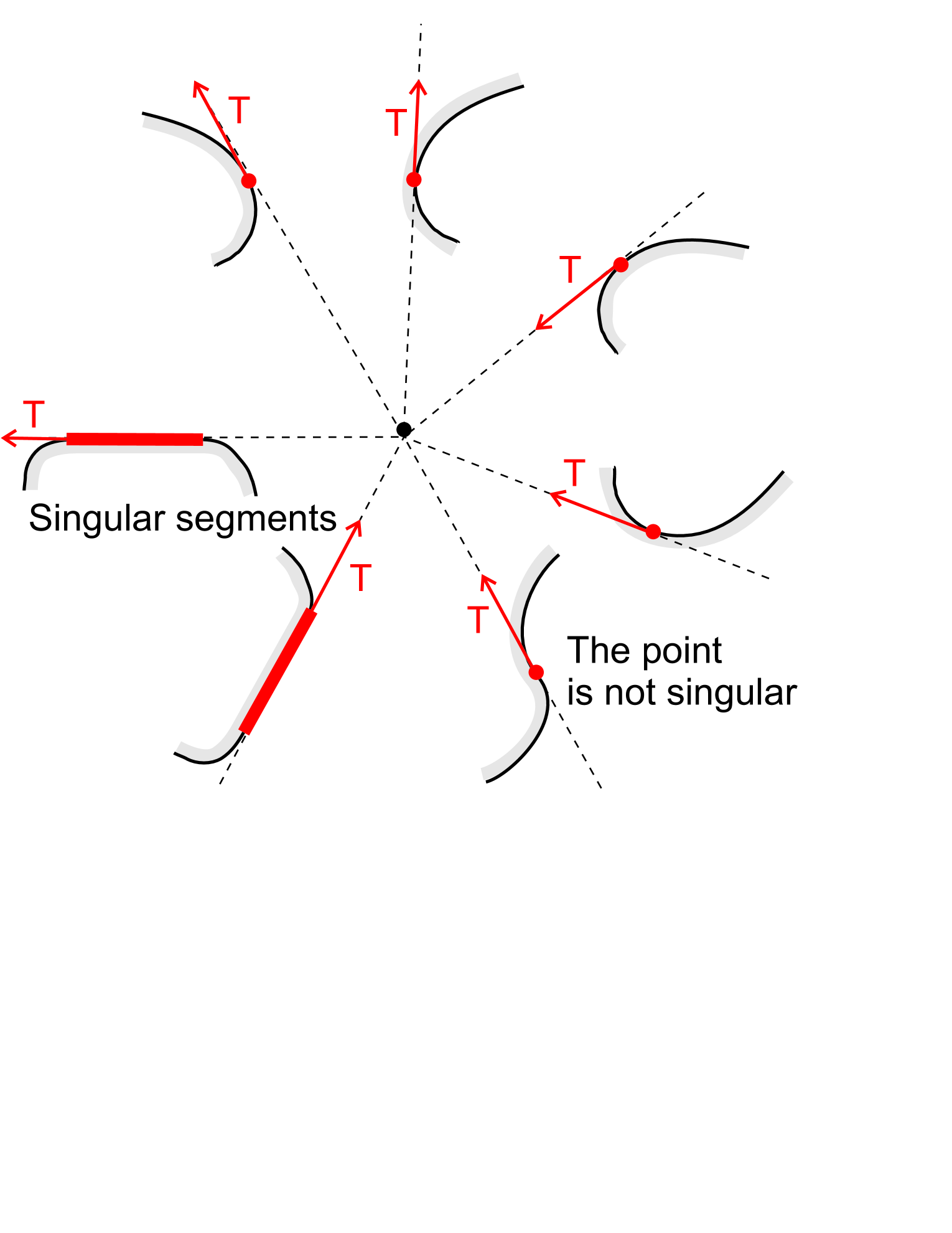
The remainder of the subsection is devoted to the proof of this claim. The notations $s,T,N,\text{\large$\mathfrak{r}$},\lambda,\zeta$ , $\varkappa$ , $\psi$ , $\varphi$ are attributed to $C=\partial\mathscr{D}$ . At the corner points of $C$ , these variables except for $s$ have one-sided limits and are assumed to instantaneously, continuously, and monotonically run between the one-sided limit values. An arc of $C$ is said to be regular if $\zeta$ (non-strictly) does not change its sign on this arc, depending on which the arc is said to be positive/negative (or $\pm$ arc). The regular arc is maximal if it cannot be extended without violation of the regularity. A connected part of $C$ and its points are said to be singular if $\zeta$ strictly changes the sign when passing it and, if this part contains more than one point, is identically zero on it; see Fig. 2(c). The singular arc is a segment of a straight line since $\varkappa\equiv 0$ on it due to (13). The ends of any maximal regular arc are singular. Due to Assumption 3 and (13), the boundary $C$ has only finitely many singular parts. A boundary point $s\in C$ is said to lie above $\mathscr{D}$ if there exists $\delta>0$ such that $((1-\delta)s,s)\subset\mathscr{D}$ and $(s,(1+\delta)s)\cap\mathscr{D}=\emptyset$ . If conversely $((1-\delta)s,s)\cap\mathscr{D}=\emptyset$ and $(s,(1+\delta)s)\subset\mathscr{D}$ , the point is said to lie below $\mathscr{D}$ .

Formulas (13) and (15) imply the following.

Observation 2.

As $s$ moves in direction $\sigma=\pm$ over a $\eta$ -arc ( $\eta=\pm$ ) of $C$ , we have $\sigma\eta\dot{\varphi}\geq 0$ . Any point of $\pm$ arc that is not singular lies above/below $\mathscr{D}$ .

Lemma 12.

As $s$ continuously moves along a regular arc, $\beta$ evolves within an interval of the form $\Delta:=[\pi k,\pi(k+1)]$ , where $k$ is an integer. When $s$ reaches a singular point, $\beta$ arrives at the end of $\Delta$ associated with the even or odd integer, depending on whether $s$ moves towards or outwards the target at this moment, respectively.

\pf

Since $\zeta$ does not change its sign, the vector $\mathfrak{r}$ does not trespass the $\lambda$ -axis, whereas $\beta$ is the polar angle of this vector. This gives rise to the first claim of the lemma. The second one is immediate from the first claim. $\quad\bullet$

Lemma 13.

Whenever SP progresses along $C$ in direction $\sigma=\pm$ , we have $\sigma\beta\geq 0$ .

\pf

This is evidently true just after any SMT. During the subsequent motion along $C$ , the inequality can be violated only at a position $s$ where $\beta=0$ and either $s$ is a corner singular point or $\varkappa(s+\sigma^{\text{\tiny$\approx$}}\!0)>0$ since $\varkappa(s+\sigma^{\text{\tiny$\approx$}}\!0)\leq 0\Rightarrow\sigma\beta(s+\sigma^{\text{\tiny$\approx$}}\!0)\geq 0$ by the third relation from (13). However, at such position, motion along $C$ is ended. $\quad\bullet$

The cave $\mathfrak{C}(s_{-},s_{+})$ is said to be positive/negative (or $\pm$ cave) if the trip from $s_{-}$ to $s_{+}$ over $\gamma_{\mathfrak{C}}$ is in the respective direction of $C$ . By Observation 2, $s$ moves from a $+$ arc to a $-$ arc in this trip and so passes a singular part of $C$ . The total number of such parts inside $\gamma_{\mathfrak{C}}$ is called the degree of the cave.^¶^¶¶Possible singular parts at the ends of $\gamma_{\mathfrak{C}}$ are not counted.

Lemma 14.

For any cave of degree $M=1$ , the arc $\gamma:=\gamma_{\mathfrak{C}}$ consists of the positive $\gamma|_{s_{-}\to s_{-}^{\ast}}$ and negative $\gamma|_{s_{+}^{\ast}\to s_{+}}$ sub-arcs and a singular part $[s_{-}^{\ast},s_{+}^{\ast}]$ . For $s\in[s_{-}^{\ast},s_{+}^{\ast}]$ , the tangential vector $T(s)$ (that is co-linear with $[\boldsymbol{\mathscr{T}},s]$ if $s$ is the corner point) is directed outwards $\boldsymbol{\mathscr{T}}$ if the cave is positive and does not contain $\boldsymbol{\mathscr{T}}$ or negative and contains $\boldsymbol{\mathscr{T}}$ . Otherwise, this vector is directed towards $\boldsymbol{\mathscr{T}}$ .

\pf

The first claim is evident. Let the cave be positive and $\boldsymbol{\mathscr{T}}\not\in\mathfrak{C}(s_{-},s_{+})$ . Suppose that $T(s)$ is directed towards $\boldsymbol{\mathscr{T}}$ . Then the same is true for $s:=s_{+}^{\ast}$ . Hence $\zeta(s_{+}^{\ast}+0)\leq 0$ and $\zeta(s_{+}^{\ast}+0)=0\Rightarrow\lambda(s_{+}^{\ast}+0)>0\Rightarrow\varkappa(s_{+}^{\ast}+^{\text{\tiny$\approx$}}\!0)>0$ since otherwise, $\zeta(s_{+}^{\ast}+^{\text{\tiny$\approx$}}\!0)\geq 0$ by (13), in violation of the definition of the singular part. In any case, $((1-\delta)s_{+}^{\ast},s_{+}^{\ast})\cap\mathscr{D}=\emptyset$ for some $\delta>0$ . Since $\boldsymbol{\mathscr{T}}\not\in\mathfrak{C}(s_{-},s_{+})$ , the segment $[0,s_{+}^{\ast})$ intersects $\gamma_{\mathfrak{C}}$ , cutting out a smaller cave $\mathfrak{C}_{\text{sm}}$ inside $\mathfrak{C}(s_{-},s_{+})$ . The singular part inside $\mathfrak{C}_{\text{sm}}$ is the second such part in the original cave, in violation of $M=1$ . This contradiction shows that $T(s)$ is directed outwards $\boldsymbol{\mathscr{T}}$ .

Now suppose that $\boldsymbol{\mathscr{T}}\in\mathfrak{C}(s_{-},s_{+})$ and $T(s)$ is directed outwards $\boldsymbol{\mathscr{T}}$ . Let a point $s_{\ast}$ moves in the positive direction along $\gamma|_{s_{+}^{\ast}\to s_{+}}$ . The ray containing $s_{\ast}$ monotonically rotates by Observation 2 and contains a continuously moving point $s^{\text{mov}}_{-}\in\gamma|_{s_{-}^{\ast}\to s_{-}}$ . As $s_{\ast}$ runs from $s_{+}^{\ast}$ to $s_{+}$ , the segment $(s^{\text{mov}}_{-},s_{\ast})$ sweeps the entire cave $\mathfrak{C}[s_{-},s_{+}]$ , and so this cave does not contain $\boldsymbol{\mathscr{T}}$ , in violation of the assumption. This contradiction proves that $T(s)$ is directed towards $\boldsymbol{\mathscr{T}}$ .

The second claim for negative caves and the third claim are established likewise. $\quad\bullet$

Lemma 15.

If SP enters a cave without the target, it leaves the cave through the other corner with $\beta\neq 0$ . In this maneuver, the direction of motion along $C$ is not changed, no point of $C$ is passed twice, and the number of SMT’s does not exceed the cave degree.

\pf

Let SP enter the cave in the positive direction; the case of the negative direction is considered likewise. The proof will be by induction on the cave degree $M$ .

Let $M=1$ . (i) Suppose first that the cave is positive and so $s$ enters it through $s_{-}$ moving over a $+$ arc. By Lemma 14, the point $s$ moves outwards the target whenever $s\in[s_{-}^{\ast},s_{+}^{\ast}]$ , and so $\beta\geq\pi$ by Lemmas 12 and 13. As $s$ moves over the subsequent $-$ arc, $\zeta$ becomes negative and so the inequality is kept true by Lemma 12. Thus $s$ leaves the cave through $s_{+}$ with $\beta\geq\pi>0$ , having made no SMT.

(ii) Let the cave be negative. Then $s$ enters it through $s_{+}$ moving over the negative arc. By Lemma 14, the point $s$ moves towards the target whenever $s\in[s_{-}^{\ast},s_{+}^{\ast}]$ . Since $\zeta(s_{+}+0)\leq 0$ , Lemma 13 yields $\beta(s_{+}+0)\geq\pi$ . By Lemma 12, $\beta\geq\pi$ until $s_{+}^{\ast}$ and so $\beta\geq 2\pi$ at $s\in[s_{-}^{\ast},s_{+}^{\ast}]$ by Lemma 14. When $s$ passes the entire $[s_{-}^{\ast},s_{+}^{\ast}]$ , the sign of $\zeta$ reverses from $-$ to $+$ and so $\beta>2\pi$ just after the passage of $s_{-}^{\ast}$ . It remains to note that $\beta\geq 2\pi>0$ while $s$ moves over the $+$ arc from $s_{-}^{\ast}$ to $s_{-}$ by Lemma 12.

Suppose that the claim of the lemma is true for any cave with degree $\leq M$ , and consider a cave of degree $M+1$ . Let this cave be positive. Then $s$ enters it through the lower corner $s_{-}$ along a positive arc. We also consider the accompanying motion of the ray containing $s$ . This ray contains a continuously moving point $s_{+}^{\circledast}\in C$ that starts at $s_{+}$ . This motion is considered until a singular part of $C$ appears on the ray segment $[s,s_{+}^{\circledast}]$ for the first time. Three cases are possible at this position.

(a) The singular part $[s_{-}^{\ast},s_{+}^{\ast}]\subset(s,s_{+}^{\circledast})$ ; see Fig. 3(a), where $s_{-}^{\ast}=s_{+}^{\ast}=:s_{\ast}$ .

By successively applying the induction hypothesis to $\mathfrak{C}(s,s_{+}^{\ast})$ and $\mathfrak{C}(s_{+}^{\ast},s^{\circledast}_{+})$ , we see that SP arrives at $s^{\circledast}_{+}$ in the positive direction and with $\beta>0$ . While $s$ moves from $s^{\ast}_{+}$ to $s_{+}$ over the $-$ arc, the vector $\text{\large$\mathfrak{r}$}(s)$ is below the $\lambda$ -axis and so $\beta\geq\pi>0$ by Lemma 12.

(b) The singular point $s_{+}^{\circledast}=s_{-}^{\ast}$ ; see Fig. 3(b), where $s_{-}^{\ast}=s_{+}^{\ast}=:s_{\ast}$ . By successively applying the induction hypothesis to $\mathfrak{C}(s,s_{\#})$ and $\mathfrak{C}(s_{\#},s^{\circledast}_{+})$ , we see that SP arrives at $s^{\circledast}_{+}$ in the positive direction and with $\beta>0$ . So $\beta(s^{\circledast}_{+})\geq 2\pi$ and SP proceeds along the $-$ arc to $s_{+}$ with $\beta\geq\pi>0$ by Lemma 12, which completes the proof.

(c) The singular point $s$ ; see Fig. 3(c). If $\beta>0$ at this point, SP enters the cave $\mathfrak{C}[s,s_{+}^{\circledast}]$ of degree $\leq M$ and by the induction hypothesis, arrives at $s_{+}^{\circledast}$ moving in the positive direction and with $\beta>0$ . If conversely $\beta=0$ , SP undergoes SMT, which cannot be terminated at the target since it does not belong to the cave at hand. So it is terminated at some point $s_{\#}\in\gamma_{\mathfrak{C}}$ . Since $\boldsymbol{\mathscr{T}}$ does not lie in the sub-cave $\mathfrak{C}(s,s_{\#})$ of the original cave, the vehicle turns right at $s_{\#}$ and thus proceeds along $C$ in the positive direction. By applying the induction hypothesis to $\mathfrak{C}(s_{\#},s^{\circledast}_{+})$ , we see that SP arrives at $s_{+}^{\circledast}$ moving in the positive direction and with $\beta>0$ in any case. The proof is completed like in the cases (a) and (b).

The case where the cave is negative is considered likewise.

Lemma 16.

Suppose that after SMT starting and ending at the points $s_{\lozenge}$ and $s_{\ast}$ , respectively, the direction of the motion along $C$ is reversed. Then the cave $\mathfrak{C}[s_{\lozenge},s_{\ast}]$ does not contain $\boldsymbol{\mathscr{T}}$ but contains the entire path traced before SMT at hand.

\pf

Let the motion direction at $s=s_{\lozenge}$ be $+$ ; the case of $-$ is considered likewise. Since on arrival at $s_{\ast}$ , the left turn is made, $\mathfrak{C}[s_{\lozenge},s_{\ast}]$ does not contain $\boldsymbol{\mathscr{T}}$ by r.3b). Suppose that the path traced before SMT at hand is not contained by this cave, i.e., the point enters this cave before. Since this cannot be done during another SMT, the point enters the cave through either $s_{\lozenge}$ or $s_{\ast}$ . In the first case, $s_{\lozenge}$ is passed twice in the opposite directions, in violation of Lemma 15. In the second case, $s_{\lozenge}$ is passed with $\beta>0$ by the same lemma and so SMT cannot be commenced. The contradiction obtained proves that the initial part of SP is inside the cave. $\quad\bullet$

Lemma 17.

If SP progresses along $C$ in a cave not containing the target, it leaves this cave through one of its corners. During this maneuver, SP passes no point of $C$ twice and makes no more SMT’s than the degree of the cave.

\pf

For the definiteness, let the cave be positive; the case of the negative cave is considered likewise. The proof will be by induction on the degree $M$ of the cave.

Let $M=1$ . We employ the notations from Lemma 14.

( $\boldsymbol{\alpha}$ ) The motion is started on $\gamma|_{s_{+}^{\ast}\to s_{-}}$ in the direction $-$ . The claim is evident.

( $\boldsymbol{\beta}$ ) The motion is started on $\gamma|_{s_{+}\to s_{+}^{\ast}}$ in the direction $-$ . Then the point necessarily arrives at $s_{+}^{\ast}$ , moving in the negative direction. Thus the situation is reduced to ( $\alpha$ ).

( $\boldsymbol{\gamma}$ ) The motion is started on $\gamma|_{s_{-}^{\ast}\to s_{+}}$ in the positive direction. The claim of the lemma is justified by the concluding arguments from (i) in the proof of Lemma 15.

( $\boldsymbol{\delta}$ ) The motion is started on $\gamma|_{s_{-}\to s_{-}^{\ast}}$ in the direction $+$ . Then the point necessarily arrives at $s_{-}^{\ast}$ , moving in the positive direction. Thus the situation is reduced to ( $\gamma$ ).

Now suppose that the claim of the lemma is true for any cave with degree $\leq M$ , and consider a cave of degree $M+1$ . Let this cave be positive for the definiteness; the case of the negative cave is considered likewise. We also consider an auxiliary motion of the point over $C$ from $s_{-}$ into the cave and the accompanying motion of the ray containing $s$ until one of the situations from Fig. 3 occurs.

Case (a) from Fig. 3. (a.1) If the motion is started on $\gamma|_{s^{\circledast}_{+}\to s_{+}}$ in direction $+$ or on $\gamma|_{s\to s_{-}}$ in direction $-$ , the claim of the lemma is justified by the concluding arguments from (i) in the proof of Lemma 15.

(a.2) If the motion is started on $\gamma|_{s_{-}^{\ast}\to s^{\circledast}_{+}}$ , the induction hypothesis applied to the cave $\mathfrak{C}[s_{-}^{\ast},s^{\circledast}_{+}]$ of degree $\leq M$ ensures that the point arrives at either $s^{\circledast}_{+}$ or $s_{-}^{\ast}$ . In the first case, it arrives in direction $+$ , thus reducing the situation to (a.1). In the second case, it arrives in direction $-$ . If $\beta\neq 0$ at this position, the point enters the cave $\mathfrak{C}[s_{-}^{\ast},s]$ in direction $-$ and afterwards leaves it through $s$ in the same direction by Lemma 15. If $\beta=0$ , SMT is commenced, which ends at the position $s$ with the left turn since $\mathfrak{C}[s_{-}^{\ast},s]$ does not contain $\boldsymbol{\mathscr{T}}$ . Hence in any case, the motion proceeds in direction $-$ from the position $s$ , which reduces the situation to (a.1).

(a.3) The case where the motion is started on $\gamma|_{s\to s_{-}^{\ast}}$ , is considered likewise.

(a.4) The cases where the motion starts on $\gamma|_{s^{\circledast}_{+}\to s_{+}}$ in direction $-$ or on $\gamma|_{s\to s_{-}}$ in direction $+$ , are trivially reduced to (a.2) and (a.3), respectively.

Case (b) from Fig. 3. (b.1) The cases where the motion starts on $\gamma|_{s^{\circledast}_{+}\to s_{+}}$ in direction $+$ or on $\gamma|_{s\to s_{-}}$ in direction $-$ , is considered like (a.1).

(b.2) If the start is on $\gamma|_{s\to s_{\#}}$ , the induction hypothesis applied to $\mathfrak{C}[s,s_{\#}]$ ensures that the point arrives at either $s$ or $s_{\#}$ . In the first case, it arrives in direction $-$ , thus reducing the situation to (b.1). In the second case, it arrives in direction $+$ and then enters the cave $\mathfrak{C}[s_{\#},s_{+}^{\circledast}]$ . By Lemma 15, the point leaves this cave through $s_{+}^{\circledast}$ in direction $+$ and with $\beta>0$ , thus reducing the situation to (b.1).

(b.3) If the motion commences on $\gamma|_{s_{\#}\to s^{\circledast}_{+}}$ , the induction hypothesis applied to the cave $\mathfrak{C}[s_{\#},s^{\circledast}_{+}]$ of degree $\leq M$ ensures that the point arrives at either $s_{\#}$ or $s^{\circledast}_{+}$ . In the first case, the arrival is in direction $-$ , after which the situation is reduced to (b.2). In the second case, the arrival is in direction $+$ . If $\beta\neq 0$ at this moment, the motion proceeds along $\gamma|_{s^{\circledast}_{+}\to s_{+}}$ in direction $+$ , and the situation is reduced to (b.1). If $\beta=0$ , SMT is commenced, which ends at the position $s$ with the left turn since the cave $\mathfrak{C}[s^{\circledast}_{+},s]$ does not contain the target. Hence the motion proceeds along $\gamma|_{s\to s_{-}}$ in direction $-$ , and the situation is still reduced to (b.1).

(b.4) The cases where the motion starts on $\gamma|_{s^{\circledast}_{+}\to s_{+}}$ in direction $-$ or on $\gamma|_{s\to s_{-}}$ in direction $+$ , are trivially reduced to (b.3) and (b.2), respectively.

Case (c) from Fig. 3. (c.1) The cases where the motion starts on $\gamma|_{s^{\circledast}_{+}\to s_{+}}$ in direction $+$ or on $\gamma|_{s\to s_{-}}$ in direction $-$ , is considered like (a.1).

(c.2) If the start is on $\gamma|_{s_{\#}\to s_{+}^{\circledast}}$ , the induction hypothesis applied to $\mathfrak{C}[s_{\#},s_{+}^{\circledast}]$ yields that the point arrives at either $s_{+}^{\circledast}$ or $s_{\#}$ . In the first case, the arrival direction is $+$ and the situation is reduced to (b.1). In the second case, the point arrives in direction $-$ and then enters $\mathfrak{C}[s_{\#},s]$ . By Lemma 15, the point leaves this cave through $s$ in direction $-$ and with $\beta>0$ . Thus we arrive at (b.1) once more.

(c.3) If the motion commences on $\gamma|_{s_{\#}\to s}$ , the induction hypothesis applied to the cave $\mathfrak{C}[s_{\#},s]$ of degree $\leq M$ ensures that the point arrives at either $s_{\#}$ or $s$ . In the first case, the arrival is in direction $+$ , after which the situation is reduced to (b.2). In the second case, the arrival is in direction $-$ , after which the situation reduces to (b.1).

(c.4) The cases where the motion starts on $\gamma|_{s^{\circledast}_{+}\to s_{+}}$ in direction $-$ or on $\gamma|_{s\to s_{-}}$ in direction $+$ , are trivially reduced to (c.2) and (c.3), respectively. $\quad\bullet$

Lemma 18.

Any part of SP where it progresses over the boundary $\partial D$ ends with SMT.

\pf

is by retracing the proof of (v) in Proposition 3.

Let $K$ be the number of singular parts of the boundary $\partial\mathscr{D}$ .

Lemma 19.

If every cave examined in r.3b) does not contain the target, SP consists of the initial $\mathscr{P}^{-}$ and terminal $\mathscr{P}^{+}$ sub-paths (some of which may contain only one point) such that each accommodates no more than $K$ SMT’s, no point of $C$ is passed twice within $\mathscr{P}^{-}$ , whereas the direction of motion along $C$ is not altered within $\mathscr{P}^{+}$ .

\pf

Suppose first that the initial position lies in some cave. Among such caves, there is one enveloping the others. By Lemma 17, SP leaves this cave and the related sub-path satisfies the properties stated in Lemma 19. If the initial position lies outside any cave, this sub-path is taken to consist of only this position. By Lemma 16, the direction of the motion along $C$ is not changed on the remaining sub-path $\mathscr{P}_{+}$ and $\mathscr{P}_{+}$ does not go inside the above maximal cave.

Suppose that within $\mathscr{P}_{+}$ , SP accommodates more than $K$ SMT’s. Any of them starts at some singular part with $\beta=0$ . Hence SP passes some singular point with $\beta=0$ at least twice and thus becomes cyclic. Now we consider the related minimal cyclic part CP of SP that starts and ends with commencing a SMT at a common point. Due to the constant direction, the closed curve CP is simple. It follows that $\sphericalangle\text{\bf TANG}\left[\text{CP}\right]=\pm 2\pi$ , whereas $\sphericalangle_{\boldsymbol{\mathscr{T}}}\text{CP}=0$ since $W=0$ for all bypassed caves and $\boldsymbol{\mathscr{T}}\not\in D$ . Hence $\sphericalangle_{0}\text{\large$\mathfrak{r}$}=\mp 2\pi$ by (14), whereas CP starts and ends with $\beta=0$ and so $\sphericalangle_{0}\text{\large$\mathfrak{r}$}=0$ . This contradiction completes the proof. $\quad\bullet$

Lemmas 18 and 19 give rise to the following.

Corollary 5.2.

If every cave examined in r.3b) does not contain $\boldsymbol{\mathscr{T}}$ , SP arrives at $\boldsymbol{\mathscr{T}}$ by making no more than $2K$ SMT’s.

Lemma 20.

If SP enters a cave containing $\boldsymbol{\mathscr{T}}$ over a positive arc with $|\beta|\leq\pi$ , it arrives at $\boldsymbol{\mathscr{T}}$ not leaving the cave. During this maneuver, no point of $C$ is passed twice and the number of SMT’s does not exceed the degree of the cave.

\pf

Let the cave be entered in direction $+$ ; the case of $-$ is considered likewise. The proof will be by induction on the degree $M$ of the cave $\mathfrak{C}[s_{-},s_{+}]$ . Since $s$ enters the cave over a positive arc, the entrance is through $s_{-}$ .

Let $M=1$ . By Lemma 14, $s$ moves towards $\boldsymbol{\mathscr{T}}$ when reaching the singular part of the cave $[s_{-}^{\ast},s_{+}^{\ast}]$ . At this position, $\beta=0$ by Lemma 12 and $\mathscr{D}$ does not obstruct the initial part of SMT, as was show in the proof of Lemma 14. So SMT is commenced. If it is not terminated at $\boldsymbol{\mathscr{T}}$ , the segment $[0,s_{-}^{\ast})$ intersects $\gamma_{\mathfrak{C}}$ , cutting out a smaller cave within the original one. The singular part inside this new cave is the second such part within the original cave, in violation of $M=1$ . Hence $\boldsymbol{\mathscr{T}}$ is reached and only one switch $\mathfrak{B}\mapsto\mathfrak{A}$ is made.

Now suppose that the conclusion of the lemma is true for any cave with degree $\leq M$ , and consider a cave of degree $M+1$ . Like in the proof of Lemma 15, we consider the motion of the ray containing $s$ until a singular point appears on the segment $[s,s_{+}^{\ast}]$ for the first time, and examine separately three possible cases depicted in Fig. 3.

(a) The singular point $s_{\ast}\in(s,s_{+}^{\ast})$ ; see Fig. 3(a). The target is contained by the cave $\mathfrak{C}[s,s_{\ast}]$ of degree $\leq M$ , which is entered in the positive direction and by Lemma 12, with $0\leq\beta\leq\pi$ . The induction hypothesis competes the proof.

(b) The singular point $s_{\ast}=s_{+}^{\ast}$ ; see Fig. 3(b). The target is evidently contained by the cave $\mathfrak{C}[s,s_{\#}]$ of degree $\leq M$ . The proof is completed like in the previous case.

(c) The singular point $s_{\ast}=s$ ; see Fig. 3(c). If at $s_{\ast}$ , the point moves outwards $\boldsymbol{\mathscr{T}}$ , the arguments from the second paragraph in the proof of Lemma 14 show that the cave does not contain $\boldsymbol{\mathscr{T}}$ , in violation of the assumption of the lemma. Hence at $s_{\ast}$ , the point moves towards $\boldsymbol{\mathscr{T}}$ and so $\beta=0$ by Lemma 12 and $\mathscr{D}$ does not obstruct the initial part of SMT, as was show in the proof of Lemma 14. Thus SMT is commenced at $s_{\ast}$ . If it is terminated at $\boldsymbol{\mathscr{T}}$ , the proof is completed. Otherwise, it arrives at $s_{\#}\in\gamma_{\mathfrak{C}}$ , as is shown in Fig. 3(c). Evidently, the cave $\mathfrak{C}[s_{\#},s]$ does not contain the target. So on reaching $s_{\#}$ , the point turns right and continues moving in the positive direction over a new positive arc and with $\beta\in[0,\pi]$ . So the proof is completed by applying the induction hypothesis to the cave $\mathfrak{C}[s_{\#},s_{+}^{\ast}]$ of degree $\leq M$ .

Proof of Proposition 11: is straightforward from Corollary 5.2 and Lemma 20.

5.3 Proof of Proposition 10.

Let $\mathscr{P}$ stand for the directed path traced by the vehicle under the control law $\mathscr{A}$ from Subsect. 5.1. We first show that after a slight modification, this path can be viewed as SP for some domain $\mathscr{D}$ provided that $\mathscr{P}$ is single (see Definition 4.4). This permits us to employ the results of Subsect. 5.2.

We use the notations $s^{-}_{i},s^{+}_{i},\gamma_{i}$ from introduced before Definition 4.4, note that for $s\in\gamma_{i}$ , the distance $d$ from the vehicle to the obstacle is a function $d=d_{i}(s)$ of $s$ , and put:

\mathscr{D}:=\Big{\{}\boldsymbol{r}:d:=\text{\bf dist}_{D}[\boldsymbol{r}]<d_{\star}(D)\;\text{an either}\;s:=\\ s(\boldsymbol{r})\in\gamma_{i}\wedge d\leq d_{i}(s)\;\text{or}\;s\not\in\cup_{i}\gamma_{i}\wedge d\leq d_{\text{trig}}\Big{\}}.

(37)

If $\sigma\dot{s}<0$ at the start of the $i$ th mode $\mathfrak{B}$ , the abscissa $s^{-}_{i}$ is passed twice during IT by Lemma LABEL:lem.sucs. For every such $i$ , the real path between these two passages is replaced by the motion along the straight line segment, which gives rise to the modified path $\mathscr{P}_{\ast}$ .

Observation 3.

Let the original path be single. The modified path $\mathscr{P}_{\ast}$ is SP for $\mathscr{D}_{\ast}$ .

Indeed, this path can be viewed as a trace of a point obeying the rules r.1)—r.5). To ensure r.3a), the direction should be pre-specified to match that of $\mathscr{P}_{\ast}$ . The property r3.b) is satisfied due to (36) and the second inequality from (7).

Lemma 21.

For a single path, the set (37) satisfies Assumption 3 and its boundary has no more than $N_{s}$ singular parts, where $N_{s}$ is completely determined by $D$ and $\boldsymbol{\mathscr{T}}$ .

\pf

The last claim in Assumption 3 holds by (7), (37). The boundary $\partial\mathscr{D}$ consists of parts traced during 1) SMT’s, 2) SMEC’s, 3) arcs of circles traced during IT’s, and 4) segments of normals to $\partial D$ resulted from the path modification.

Any part 1) clearly satisfies Assumption 3 and is either singular or does not contain singular points; their number does not exceed $(P+1)(Q+1)$ by Lemma 9.

Since parts 2) are separated by SMT’s, their number does not exceed $(P+1)(Q+1)+1$ . Any part 2) lies on a $d$ -equidistant curve $C(d)$ with $d\leq d_{\text{trig}}$ . Due to (8), $\zeta_{C(d)}(s)=\zeta_{\partial D}(s)+d$ , Assumption 3 holds since the boundary $\partial D$ is piece-wise analytical, and the singular parts of $C(d)$ are the connected components of the set from Corollary 4.2. So type 2) arcs of $C$ accommodate no more than $F[(P+1)(Q+1)+1]$ singular parts.

It remains to note that parts 3) and 4) do not contain singular points since $\beta$ monotonically evolves from $0$ during IT’s.

Lemma 22.

If the vehicle finds the target in $\mathfrak{C}_{\mathfrak{A}^{\dagger}}$ after some occurrence $\mathfrak{A}^{\dagger}$ of mode $\mathfrak{A}$ , it arrives at the target by making after this no more than $N_{s}$ switches $\mathfrak{A}\mapsto\mathfrak{B}$ .

\pf

Let us consider a part $\mathscr{P}$ of the path that starts in mode $\mathfrak{B}$ preceding $\mathfrak{A}^{\dagger}$ . Suppose first that this part is not single and truncate it from the right, leaving its maximal single sub-part $\mathscr{P}^{\dagger}$ . The terminal position of $\mathscr{P}^{\dagger}$ lies on a previously passed piece of $\mathscr{P}^{\dagger}$ . Let $\mathscr{D}^{\dagger}$ and $\mathscr{P}^{\dagger}_{\ast}$ be the related domain (37) and modified path. Associated with $\mathfrak{C}_{\mathfrak{A}^{\dagger}}$ is a cave of $\mathscr{D}^{\dagger}$ into which $\mathscr{P}^{\dagger}_{\ast}$ turns with $|\beta|\leq\pi$ . By Lemma 20, $\mathscr{P}^{\dagger}_{\ast}$ cannot arrive at a previously passed point, in violation of the above property. This contradiction proves that the entire path $\mathscr{P}$ is single. Then Lemmas 20 and 21 guarantee that $\mathscr{P}_{\ast}$ arrives at $\boldsymbol{\mathscr{T}}$ by making no more than $N_{s}$ SMT’s. It remains to note that $\mathscr{P}$ and $\mathscr{P}_{\ast}$ arrive at $\boldsymbol{\mathscr{T}}$ only simultaneously, and each occurrence of $\mathfrak{A}$ gives rise to a SMT in $\mathscr{P}_{\ast}$ .

Lemma 23.

After no more than $N_{s}+1$ switches $\mathfrak{A}\mapsto\mathfrak{B}$ , the direction in which $s$ moves along $\partial D$ within modes $\mathfrak{B}$ is not altered.

\pf

Consider an occurrence $\mathfrak{A}^{\dagger}$ of mode $\mathfrak{A}$ after which the direction is altered and the path $\mathscr{P}$ from the start of the entire motion until the end of $\mathfrak{A}^{\dagger}$ . Suppose that $\mathscr{P}$ is not single and truncate it from the left, leaving the maximal single part $\mathscr{P}^{\dagger}$ . The starting point of $\mathscr{P}^{\dagger}$ is passed once more within $\mathscr{P}^{\dagger}$ , both times in mode $\mathfrak{B}$ . So this double point is inherited by $\mathscr{P}^{\dagger}_{\ast}$ , where $\mathscr{D}^{\dagger}$ and $\mathscr{P}^{\dagger}_{\ast}$ are the related domain (37) and modified path. Associated with $\mathfrak{C}_{\mathfrak{A}^{\dagger}}$ is a cave $\mathfrak{C}_{\mathscr{D}^{\dagger}}$ of $\mathscr{D}^{\dagger}$ ; these two sets contain the target only simultaneously due to (7). Hence $\mathscr{P}$ and $\mathscr{P}^{\dagger}_{\ast}$ acquire a common turn direction at their ends. So SP $\mathscr{P}^{\dagger}_{\ast}$ has converse directions of motion along the boundary at the start and end of the last involved SMT and by Lemmas 16 and 17, has no double points. This contradiction proves that the entire $\mathscr{P}^{\dagger}$ is single. Due to Lemma 16, the modified path $\mathscr{P}_{\ast}^{\dagger}$ lies in $\mathfrak{C}_{\mathscr{D}^{\dagger}}$ and so involves no more than $N_{s}$ SMT’s thanks to Lemmas 17 and 21. It remains to note that each occurrence of $\mathfrak{A}$ gives rise to a SMT in $\mathscr{P}_{\ast}$ . $\quad\bullet$

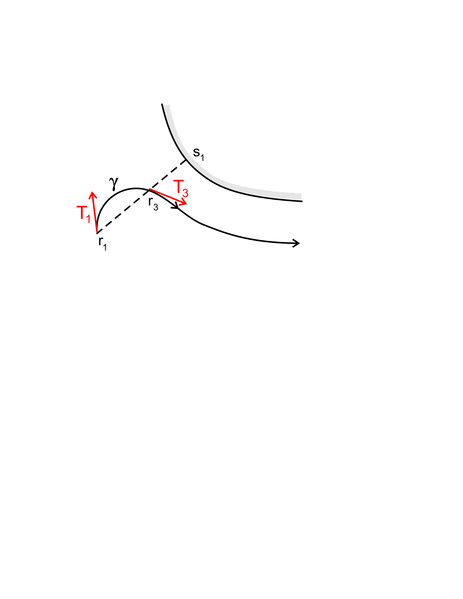
To prove Proposition 10, it in fact remains to show that the vehicle cannot pass more than $N_{s}$ modes $\mathfrak{A}$ in a row, constantly not finding the target in $\mathfrak{C}_{\mathfrak{A}}$ and not changing the direction of the motion along $\partial D$ . The next lemma with corollaries serves this proof. The symbol $\angle(a,b)\in(-\pi,\pi]$ stands for the angle from the vector $a$ to $b$ . Let the points $\boldsymbol{r}_{i},i=1,2$ on $\mathscr{P}$ be at the distance $\text{\bf dist}_{D}[\boldsymbol{r}_{i}]\leq d_{\text{trig}}$ and such that when traveling between them, the path does not intersect itself and except for $\boldsymbol{r}_{i}$ , has no points in common with the normals $[\boldsymbol{r}_{i},s_{i}]$ , where $s_{i}:=s[\boldsymbol{r}_{i}]$ . The points $s_{i}$ split $\partial D$ into two curves. Being concatenated with the above normals and $\mathscr{P}|_{\boldsymbol{r}_{1}\to\boldsymbol{r}_{2}}$ , they give rise to Jordan loops, with one of them enveloping the other. Let $\gamma_{\text{inner}}$ be the curve giving rise to the inner loop LOOP, and $\sigma=\pm$ be the direction from $s_{1}$ to $s_{2}$ along $\gamma_{\text{inner}}$ .

Lemma 24.

If LOOP does not encircle the target, the following relation holds

\sphericalangle_{0}\text{\large$\mathfrak{r}$}_{\mathscr{P}}|_{\boldsymbol{r}_{1}\to\boldsymbol{r}_{2}}=\sphericalangle_{0}\text{\large$\mathfrak{r}$}_{\partial D}|_{s_{1}\xrightarrow{\sigma}s_{2}}+\sphericalangle_{\boldsymbol{\mathscr{T}}}[\boldsymbol{r}_{1},s_{1}]-\sphericalangle_{\boldsymbol{\mathscr{T}}}[\boldsymbol{r}_{2},s_{2}]\\ +\angle\left[\sigma T_{\partial D}(s_{1}),T_{\mathscr{P}}(\boldsymbol{r}_{1})\right]-\angle\left[\sigma T_{\partial D}(s_{2}),T_{\mathscr{P}}(\boldsymbol{r}_{2})\right].

(38)

\pf

Let $\sigma=+$ ; $\sigma=-$ is considered likewise. By applying the Hopf’s theorem to LOOP, we see that

\sphericalangle_{\boldsymbol{\mathscr{T}}}[s_{1},\boldsymbol{r}_{1}]+\sphericalangle_{\boldsymbol{\mathscr{T}}}\mathscr{P}|_{\boldsymbol{r}_{1}\to\boldsymbol{r}_{2}}+\sphericalangle_{\boldsymbol{\mathscr{T}}}[\boldsymbol{r}_{2},s_{2}]-\sphericalangle_{\boldsymbol{\mathscr{T}}}\partial D_{s_{1}\to s_{2}}=0,\\ \sphericalangle\text{\bf TANG}\left[\mathscr{P}|_{\boldsymbol{r}_{1}\to\boldsymbol{r}_{2}}\right]=\sphericalangle\text{\bf TANG}\left[\partial D_{s_{1}\to s_{2}}\right]\\ -\angle\left[T_{\partial D}(s_{1}),T_{\mathscr{P}}(\boldsymbol{r}_{1})\right]+\angle\left[T_{\partial D}(s_{2}),T_{\mathscr{P}}(\boldsymbol{r}_{2})\right].

The proof is completed by the second formula in (14). $\quad\bullet$

The next claim employs the notations introduced at the beginning of Subsect. 5.1.

Corollary 5.3.

Suppose that $\boldsymbol{\mathscr{T}}\not\in\mathfrak{C}_{\mathfrak{A}^{\dagger}}$ and the value of $\sigma$ maintained during the occurrence $\mathfrak{A}^{\dagger}$ of mode $\mathfrak{A}$ is not altered when $\mathfrak{A}^{\dagger}\mapsto\mathfrak{B}$ . Then (38) holds with $\boldsymbol{r}_{1}:=\boldsymbol{r}_{\lozenge},\boldsymbol{r}_{2}:=\boldsymbol{r}_{\ast}$ .

This is true since in this claim and Lemma 24, $\sigma$ is the same.

Corollary 5.4.

Let $\boldsymbol{r}_{1}$ and $\boldsymbol{r}_{2}$ be successively passed within a common mode $\mathfrak{B}$ , where $\sigma(t)\equiv\sigma=\pm$ . If $\boldsymbol{r}_{2}$ is passed after IT, (38) holds, where $\sphericalangle_{0}\text{\large$\mathfrak{r}$}_{\partial D}|_{s_{1}\xrightarrow{\sigma}s_{2}}$ accounts for the entire motion of the projection $s=s[\boldsymbol{r}],\boldsymbol{r}\in\mathscr{P}_{\boldsymbol{r}_{1}\to\boldsymbol{r}_{2}}$ , including possible full runs over $\partial D$ .

If 1) $s$ does not run over the entire $\partial D$ and 2) either $\boldsymbol{r}_{1}$ is passed after IT or $\text{\rm sgn}\dot{s}=\sigma$ at the start of the mode, the claim is evident. If 1) holds but 2) does not, the path may intersect $[s_{1},\boldsymbol{r}_{1}]$ and so direct application of Lemma 24 is impossible. Then we apply this lemma to $\boldsymbol{r}_{1}:=\boldsymbol{r}_{3}$ , where $\boldsymbol{r}_{3}$ is the point where the vehicle intersects the normal for the second time during IT; see Fig. 4. The proof is completed by noting that $\sphericalangle_{\boldsymbol{\mathscr{T}}}[\boldsymbol{r}_{1},\boldsymbol{r}_{3}]=\sphericalangle_{\boldsymbol{\mathscr{T}}}\gamma,\sphericalangle\text{\bf TANG}\left[\gamma\right]=\angle[T_{1},T_{3}]$ and so $\sphericalangle_{0}\text{\large$\mathfrak{r}$}_{\mathscr{P}}|_{\boldsymbol{r}_{1}\to\boldsymbol{r}_{3}}=\sphericalangle_{0}\text{\large$\mathfrak{r}$}_{\gamma}=\sphericalangle_{\boldsymbol{\mathscr{T}}}[\boldsymbol{r}_{1},\boldsymbol{r}_{3}]-\angle[T_{1},T_{3}]$ , as well as that $\angle\left[\sigma T_{\partial D}(s_{1}),T_{3}\right]=\angle\left[\sigma T_{\partial D}(s_{1}),T_{1}\right]+\angle[T_{1},T_{3}]$ . The claim is generalized on the case where 1) is not true by proper partition of the path, followed by summation of the formulas related to the resultant pieces.

Corollary 5.5.

Let points $\boldsymbol{r}_{1}$ and $\boldsymbol{r}_{2}$ be successively passed in modes $\mathfrak{B}$ (maybe, different). Suppose that $\boldsymbol{r}_{2}$ is not attributed to IT and when traveling from $\boldsymbol{r}_{1}$ to $\boldsymbol{r}_{2}$ , the vehicle constantly does not find the target in $\mathfrak{C}_{\mathfrak{A}}$ and does not change $\sigma$ . Then (38) holds, where $\sphericalangle_{0}\text{\large$\mathfrak{r}$}_{\partial D}|_{s_{1}\xrightarrow{\sigma}s_{2}}$ accounts for the entire motion of the projection $s=s[\boldsymbol{r}],\boldsymbol{r}\in\mathscr{P}_{\boldsymbol{r}_{1}\to\boldsymbol{r}_{2}}$ , including possible full runs over $\partial D$ .

It is assumed that as the vehicle moves in mode $\mathfrak{A}$ , the projection $s$ continuously and monotonically goes over $\partial D$ from $s_{\lozenge}$ to $s_{\ast}$ in the direction $\sigma$ .

Lemma 25.

The vehicle cannot pass more than $N_{s}$ modes $\mathfrak{A}$ in a row, constantly not finding the target in $\mathfrak{C}_{\mathfrak{A}}$ and not changing the direction of the motion along $\partial D$ .

\pf

Suppose the contrary and that $\sigma=+$ ; the case $\sigma=-$ is considered likewise. By Observation 1, the $i$ th mode $\mathfrak{A}^{i}$ in the row starts when $s$ lies in an $+$ exit arc $A^{i}$ , whereas $\zeta\geq 0$ when it ends. Hence $A^{1},A^{2},\ldots$ cannot repeat until $s$ completes the full run over $\partial D$ . However, they do repeat since the number of $+$ arcs does not exceed $F$ by Observation 1, and $F\leq N_{s}$ by construction from the proof of Lemma 21. Hence the path $\mathscr{P}$ can be truncated so that the first and last modes $\mathfrak{A}$ start at positions $\boldsymbol{r}_{1}$ and $\boldsymbol{r}_{2}$ , respectively, lying on a common $+$ exit arc $A$ , whereas $s$ encircles the entire boundary $\partial D$ during the move over the truncated $\mathscr{P}$ . By the definition of the $+$ arc, $\text{\large$\mathfrak{r}$}_{\partial D}(s)$ evolves within the fourth quadrant as $s$ runs from $s_{1}$ to $s_{2}$ within the $+$ arc and so the absolute value of its turning angle does not exceed $\pi/2$ . This and (17) (where $d_{\ast}:=0$ ) imply that $\sphericalangle_{0}\text{\large$\mathfrak{r}$}_{\partial D|_{s_{1}\to s_{2}}}\leq-3/2\pi$ . In (38), $|\sphericalangle_{\boldsymbol{\mathscr{T}}}[\boldsymbol{r}_{i},s_{i}]|<\pi/2$ and $\angle\left[T_{\partial D}(s_{i}),T_{\mathscr{P}}(\boldsymbol{r}_{i})\right]=0$ since the segments $[\boldsymbol{r}_{i},s_{i}]$ and $[\boldsymbol{r}_{i},\boldsymbol{\mathscr{T}}]$ are perpendicular. Overall, (38) implies that

\sphericalangle_{0}\text{\large$\mathfrak{r}$}_{\mathscr{P}|_{\boldsymbol{r}_{1}\to\boldsymbol{r}_{2}}}<-\frac{\pi}{2}.

(39)

The path $\mathscr{P}|_{\boldsymbol{r}_{1}\to\boldsymbol{r}_{2}}$ starts with $\beta=0$ and whenever $\beta=0$ is encountered, the angle $\beta$ may stay constant during SMT but after this SMT $\beta$ becomes positive by (16) (see Fig. 2(b)) since the robot turns right. The last claim holds thanks to (iii) of Proposition 3 if $\mathfrak{B}$ is not terminated during this SMT and (36) otherwise. Such behavior of $\beta$ is inconsistent with (39). The contradiction obtained completes the proof. $\quad\bullet$

Proof of Proposition 10 is straightforward from (v) of Proposition 3 and Lemmas 22, 23, and 25.

5.4 Proof of (ii) in Theorem 1.

Let $P_{k}$ be the probability that the vehicle does not arrive at $\boldsymbol{\mathscr{T}}$ after making $kN$ switches $\mathfrak{A}\to\mathfrak{B}$ , where $N$ is taken from Proposition 10. Given a realization of $\sigma$ ’s for the first $kN$ switches, the probability of the $(k+1)$ th event does not exceed the probability $P_{\ast}$ that the next $N$ realizations are not identical to those generated by the algorithm $\mathscr{A}$ for the related initial state. Here $P_{\ast}\leq\rho$ , where $\rho:=1-\min\{p,1-p\}^{N}$ and $p$ is the probability of picking $+$ in (4). So the law of total probability yields that $P_{k+1}\leq\rho P_{k}\Rightarrow P_{k}\leq\rho^{k-1}P_{1}\to 0$ as $k\to\infty$ . It remains to note that the probability not to achieve $\boldsymbol{\mathscr{T}}$ does not exceed $P_{k}$ for any $k$ .

6 Proof of (ii) in Theorem 1 and Theorem 2

For the definiteness, we consider the vehicle driven by the basic algorithm with the right turns. So in any SMEC the vehicle has the obstacle to the left. The proof basically follows that from the previous section and employs many facts established there. The difference is that now we do not need to introduce an auxiliary deterministic algorithm since the examined one is deterministic itself.

As before, we first consider another obstacle $\mathscr{D}\not\ni\boldsymbol{\mathscr{T}}$ satisfying Assumption 3. Let a point $\boldsymbol{r}$ moves in the plane according to the following rules:

r.1)

If $\boldsymbol{r}\not\in\mathscr{D}$ , $\boldsymbol{r}$ moves to $\boldsymbol{\mathscr{T}}$ in a straight line; $\boldsymbol{r}(0)\not\in\mathscr{D}$ ;
r.2)

If $\boldsymbol{r}$ hits $C:=\partial\mathscr{D}$ , it turns right and then moves in the positive direction along the boundary, counting the angle $\beta$ ;
r.3)

This motion lasts until $\beta=0$ and new SMT is possible;
r.4)

The point halts as soon as it arrives at the target.

The path traced by $\boldsymbol{r}$ is called the symbolic path (SP). Any SMT according to r.1) except for the first one starts and ends at some points $s_{\lozenge},s_{\ast}\in C$ , which cut out a cave $\mathfrak{C}[s_{\lozenge},s_{\ast}]$ .

We start with noting that the following specification of Observation 2 now holds.

Observation 4.

As $\boldsymbol{r}$ moves over a $\pm$ -arc of $C$ , we have $\pm\dot{\varphi}\geq 0$ . Non-singular points of $\pm$ -arc lie above/below $\mathscr{D}$ .

Lemma 12 evidently remains valid, whereas Lemma 13 holds in the following specified form.

Lemma 26.

Whenever SP lies on $C$ , we have $\beta\geq 0$ .

It is easy to see by inspection that Lemma 15 remains true as well, where in the case from Fig. 3 the right turn at the point $s_{\#}$ is justified by not the absence of the target in the cave but the very algorithm statement. The following claim is analog of Lemma 16

Lemma 27.

Suppose that after SMT starting and ending at the points $s_{\lozenge}$ and $s_{\ast}$ , respectively, SP enters the cave $\mathfrak{C}[s_{\lozenge},s_{\ast}]$ . The this cave contains the entire path traced before SMT at hand.

\pf

The proof is be retracing the arguments from the proof of Lemma 16 with the only alteration: the point cannot enter the cave through $s_{\lozenge}$ since this violates the always positive direction of motion along the boundary. $\quad\bullet$

Now we revert to the vehicle at hand and show that Lemma 27 extends on the directed path $\mathscr{P}$ traced by this vehicle. The next lemma employs the notations $\mathfrak{A}^{\dagger}$ and $\sigma_{\mathfrak{A}^{\dagger}}$ introduced at the beginning of subsection 5.1.

Lemma 8.

^a For any occurrence $\mathfrak{A}^{\dagger}$ of mode $\mathfrak{A}$ that holds between two modes $\mathfrak{B}$ , we have $\sigma_{\mathfrak{A}^{\dagger}}=+$ .

\pf

Suppose to the contrary that $\sigma_{\mathfrak{A}^{\dagger}}=-$ . Then according to the ’only-right-turns’ option of the algorithm, the vehicle enters the cave $\mathfrak{C}_{\mathfrak{A}^{\dagger}}$ after termination of $\mathfrak{A}^{\dagger}$ . We are going to show that then similar to Lemma 16, this cave contains the entire path passed by the vehicle until this moment and so its initial location. Due to the first relation from (7), the last claim implies that the initial location $\boldsymbol{r}_{0}$ is also contained by a cave of $N(d_{\text{trig}})$ , in violation of the assumptions of Theorem 2. This contradiction will complete the proof.

Thus it remains to show that $\mathfrak{C}_{\mathfrak{A}^{\dagger}}$ does contain the path traced so far. Suppose the contrary. Since in the mode $\mathfrak{B}$ preceding $\mathfrak{A}^{\dagger}$ , the vehicle has the obstacle to the left, it passes to $\mathfrak{A}^{\dagger}$ from inside the cave. It follows that the moment after $\mathfrak{A}^{\dagger}$ is not the first time when the vehicle enters the cave. Let us consider the last of these ’preceding’ enters and the path $\mathscr{P}$ traced by the vehicle since this moment until the commencement of $\mathfrak{A}^{\dagger}$ . By combining Lemma 15 with the arguments from the proof of Lemma 22, we conclude that this path is single and $\beta>0$ at its end, which makes mode $\mathfrak{A}^{\dagger}$ impossible. The contradiction obtained completes the proof. $\quad\bullet$

This lemma entails that Corollaries 5.3, 5.4, and 5.5 remain true in the following specified forms.

Corollary 6.1.

For $\boldsymbol{r}_{1}=\boldsymbol{r}_{\lozenge},\boldsymbol{r}_{2}=\boldsymbol{r}_{\ast}$ , (38) holds with $\sigma\!=\!+$ .

Corollary 6.2.

Let $\boldsymbol{r}_{1},\boldsymbol{r}_{2}$ be successively passed within a common mode $\mathfrak{B}$ . If $\boldsymbol{r}_{2}$ follows IT, (38) holds with $\sigma=+$ and $\sphericalangle_{0}\text{\large$\mathfrak{r}$}_{\partial D}|_{s_{1}\xrightarrow{\sigma}s_{2}}$ accounting for possible full runs over $C$ .

Corollary 6.3.

Suppose that points $\boldsymbol{r}_{1}$ and $\boldsymbol{r}_{2}$ are successively passed in modes $\mathfrak{B}$ (maybe, different) and $\boldsymbol{r}_{2}$ is not attributed to IT. Then (38) holds with $\sigma=+$ , where $\sphericalangle_{0}\text{\large$\mathfrak{r}$}_{\partial D}|_{s_{1}\xrightarrow{\sigma}s_{2}}$ accounts for the entire motion of the projection $s=s[\boldsymbol{r}],\boldsymbol{r}\in\mathscr{P}_{\boldsymbol{r}_{1}\to\boldsymbol{r}_{2}}$ , including possible full runs over $\partial D$ .

We also note that at the moment when a SMEC ends, $s\in S_{0}:=\{s\in\partial D:-d_{\text{trig}}\leq\zeta_{\partial D}(s)<0,\lambda_{\partial D}(s)>0\}$ . Since the boundary is piece-wise analytical, this set has finitely many connected components (called exit arcs).

PROOF OF THEOREM 2 This proof retraces many arguments from the proof of Lemma 25. Suppose the contrary and that the vehicle does not arrive at the target. Then the projection $s$ repeatedly encircles the boundary. (This includes the imaginary moves of $s$ when the vehicle is in mode $\mathfrak{A}$ .) By retracing the arguments from the proof of (v) in Proposition 3, we conclude that the path $\mathscr{P}$ can be truncated so that the first and last modes $\mathfrak{A}$ start at positions $\boldsymbol{r}_{1}$ and $\boldsymbol{r}_{2}$ , respectively, lying on a common exit arc $A$ , whereas $s$ encircles the entire boundary $\partial D$ during the move over the truncated $\mathscr{P}$ . By the definition of the exit arc, $\text{\large$\mathfrak{r}$}_{\partial D}(s)$ evolves within the fourth quadrant as $s$ runs from $s_{1}$ to $s_{2}$ within the $+$ arc and so the absolute value of its turning angle does not exceed $\pi/2$ . This and (17) (where $d_{\ast}:=0$ ) imply that $\sphericalangle_{0}\text{\large$\mathfrak{r}$}_{\partial D|_{s_{1}\to s_{2}}}\leq-3/2\pi$ . In (38), $|\sphericalangle_{\boldsymbol{\mathscr{T}}}[\boldsymbol{r}_{i},s_{i}]|<\pi/2$ and $\angle\left[T_{\partial D}(s_{i}),T_{\mathscr{P}}(\boldsymbol{r}_{i})\right]=0$ since the segments $[\boldsymbol{r}_{i},s_{i}]$ and $[\boldsymbol{r}_{i},\boldsymbol{\mathscr{T}}]$ are perpendicular. Overall, (38) implies (39). The path $\mathscr{P}|_{\boldsymbol{r}_{1}\to\boldsymbol{r}_{2}}$ starts with $\beta=0$ and whenever $\beta=0$ is encountered, the angle $\beta$ may stay constant during SMT but after this SMT $\beta$ becomes positive since the robot turns right. The last claim holds thanks to (iii) of Proposition 3 if $\mathfrak{B}$ is not terminated during this SMT and the right-turn option in (4) otherwise. Such behavior of $\beta$ is inconsistent with (39). The contradiction obtained completes the proof. $\quad\bullet$

PROOF OF (ii) IN THEOREM 1 This claim is immediate from Theorem 2. $\quad\bullet$

References

[1] D. Thompson, On Growth and Form, Cambridge University Press, Cambridge, 1966.
[2] J. Camhi, E. Johnson, High-frequency steering maneuvers mediated by tactile cues: Antennal wall-following in the cockroach, The Journal of Experimental Biology 202 (1999) 631 643.
[3] B. Fajen, Steering toward a goal by equalizing taus, Journal of Experimental Psychology: Human Perception and Performance 27 (4) (2001) 953–968.
[4] H. Abelson, A. A. diSessa, Turtle Geometry, MIT Press, Cambridge, 1980.
[5] V. Lumelsky, S. Tiwari, An algorithm for maze searching with azimuth input, in: Proceedings of the IEEE Conference on Robotics and Automation, San Diego, CA, 1991, pp. 111 –116.
[6] V. I. Utkin, Sliding Modes in Control Optimization, Springer-Verlag, Berlin, 1992.
[7] E. Kreiszig, Differential Geometry, Dover Publications, Inc., NY, 1991.
[8] A. Matveev, M. Hoy, A. Savkin, Mixed nonlinear-sliding mode control of an unmanned farm tractor in the presence of sliding, in: Proceedings of the 11th International Conference on Control, Automation, Robotics and Vision, Singapore, 2010, pp. 927–932.