Propagation of gamma rays and production of free electrons in air
Abstract
A new concept of remote detection of concealed radioactive materials has been recently proposed [1]-[3]. It is based on the breakdown in air at the focal point of a high-power beam of electromagnetic waves produced by a THz gyrotron. To initiate the avalanche breakdown, seed free electrons should be present in this focal region during the electromagnetic pulse. This paper is devoted to the analysis of production of free electrons by gamma rays leaking from radioactive materials. Within a hundred meters from the radiation source, the fluctuating free electrons appear with the rate that may exceed significantly the natural background ionization rate. During the gyrotron pulse of about 10 microsecond length, such electrons may seed the electric breakdown and create sufficiently dense plasma at the focal region to be detected as an unambiguous effect of the concealed radioactive material.
1 Introduction
A new concept of remote detection of concealed radioactive materials has been recently proposed [1]. This concept is based on breakdown in free air at the focal point of a high-power beam of electromagnetic waves. To realize such breakdown, the wave amplitude in a focal region should exceed the breakdown threshold. To initiate the avalanche breakdown process, seed free electrons should be present in this focal region during the electromagnetic pulse. When the wavelength is short enough (sub-THz or THz frequency range) the wave beam can be focused in a spot with dimensions on the order of a wavelength and, then, the total volume where the wave amplitude exceeds the breakdown threshold can be rather small. This fact allows one to realize conditions [1] when the breakdown rate in the case of the ambient electron density is rather low. So in the cases when the breakdown rate is much higher than the expected one can conclude that in the vicinity of a focused wave beam there is a hidden source of radioactive material which ionizes the air. Some issues important for realizing this concept are discussed in Refs. [2] and [3].
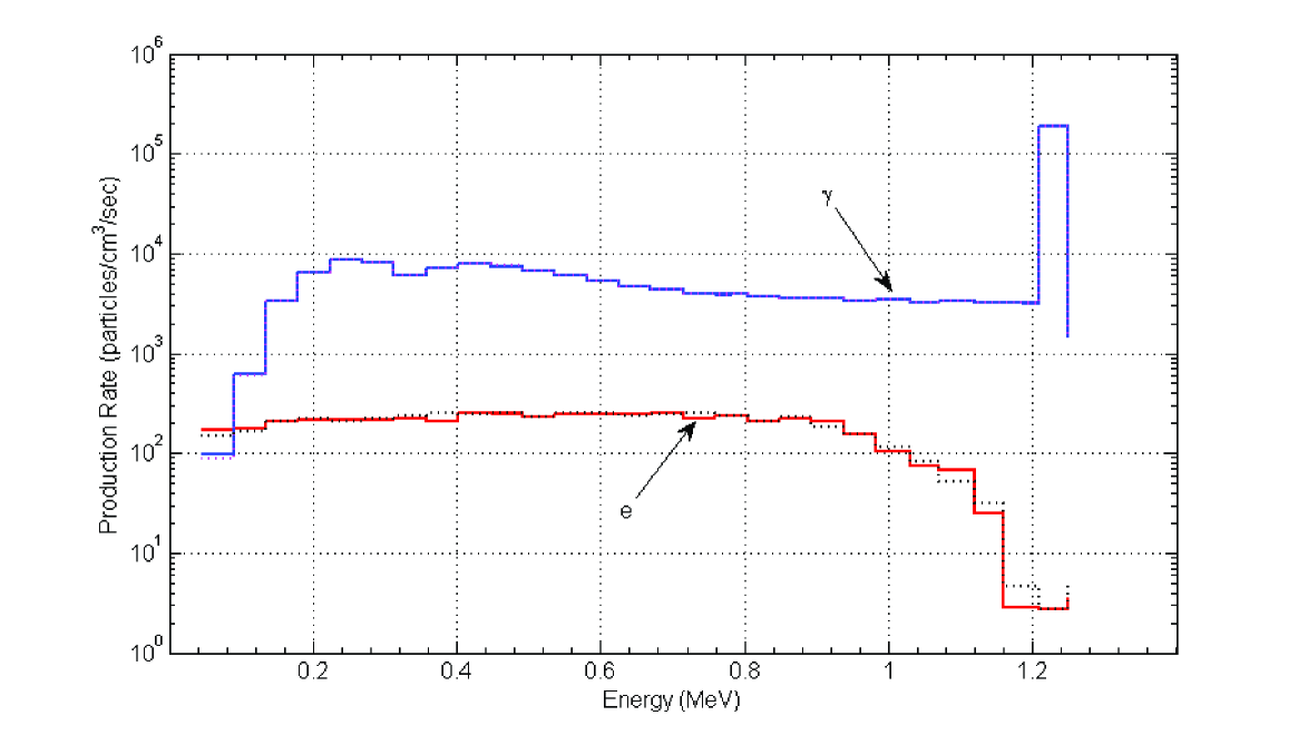
In the present paper, we analyze another issue important for realizing this concept which was only briefly discussed in previous references, viz. propagation of -rays in air and production of free electrons by these quanta, mainly due to inelastic Compton scattering. It should be noted that, in principle, due to the atomic reaction radioactive materials emit both MeV-scale -rays and -electrons. For example, a disintegrating atom of Co produces one MeV -electron and two -quanta with the energies and MeV [5]. Metal shielding and container walls largely stop -electrons, while absorbing only a fraction of -rays. All unabsorbed -rays, even scattered ones, will eventually leak through the walls and propagate in air. An example of energy distribution of -rays and electrons outside the container wall is shown in Fig. 1 reproduced from Ref. [2].
The energetic -quanta escaped from the container will occasionally collide with air molecules, experiencing Compton scattering and photoelectric absorption, as discussed below. Their propagation distance can be estimated based on the interaction cross-section given, e.g., in Ref. [4] on Figures 2.50 (d) and (e) for nitrogen and oxygen, respectively. (One of these very similar figures was reproduced in Ref. [2].) From these figures one can draw, at least, two conclusions. First, for energies between 0.1 MeV and 1.2 MeV shown in Fig. 1, the dominant effect in the production of free electrons is the Compton scattering (this conclusion agrees with Figures 2.42, 2.43 of Ref. [4]). Second, the interaction cross-section , as the function of energy, gradually increases from about 0.055 cm2/g at 1.2 MeV to about 0.16 cm2/g at 0.1 MeV. Correspondingly, the mean free pass of -rays in air (atoms/cm3) defined as varies from 120 m for 1.2 MeV quanta down to about 40 m for 100 keV quanta. When the energy of -quanta decreases down to 30 keV and below, the photoelectric absorption becomes the dominant effect.
It is important that both the Compton scattering and photoelectric absorption ionize air molecules, producing high-energy electrons within the MeV range. These primary electrons, which should not be confused with the -electrons directly from radioactivity, cannot propagate too far: they will be absorbed by air within a few meters [4]. During their short lifetime, however, most of these primary electrons produce thousands of secondary ones. It is this process that determines the local rate of total electron production required for the avalanche breakdown [3]. As discussed above, all unabsorbed -quanta propagate away from the radioactive source, continuing to produce free electrons. Hence to estimate the total rate of free-electron production at various distances from the radioactive source, one needs to analyze the collisional propagation of -quanta in air. In this paper, we analyze the photon propagation in the near-source zone, i.e., at distances less or of order of the mean free pass estimated above.
![[Uncaptioned image]](https://cdn.awesomepapers.org/papers/f72ccc62-e1d1-4a85-b1a1-21b9cb83f105/x2.png)
![[Uncaptioned image]](https://cdn.awesomepapers.org/papers/f72ccc62-e1d1-4a85-b1a1-21b9cb83f105/x3.png)
2 Production of free electrons
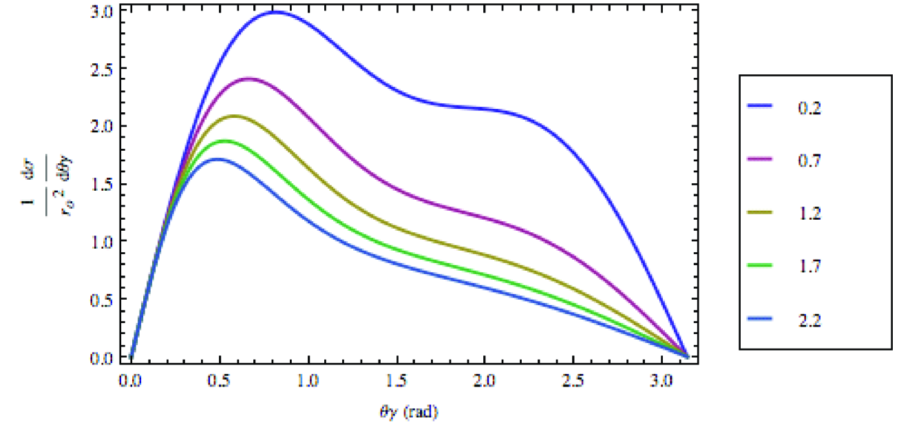
As propagating -quanta collide with air molecules, producing high-energy primary electrons, they experience a strong angular scatter and energy losses. The major electron production takes place when the photon energy remains between 30 keV and 1.3 MeV, i.e., in the energy range where the Compton scattering dominates. In this range, one can successfully apply the Klein-Nishina (K-N) theory that describes Compton scattering of photons by free electrons [4]. Indeed, after a typical collision between the incident photon and an electron bound within an O2 or N2 molecule, the originally bound electron becomes free and acquires a significant momentum (energy). If the acquired energy greatly exceeds the electron binding energy then both the scattered photons and released electrons will have momentum distributions fairly close to those if the originally bound electron was free and at rest. Furthermore, if the incident-photon energy is well above the maximum electron binding energy (the K-shell edge), eV for the air molecules, then the K-N theory should be applicable to all bound electrons with the exception of small-angle scattering when the released electrons acquire a small energy, [4, Section 2.6.2.1].
As described in numerous textbooks, see, e.g., Ref. [4, Section 2.6], in the frameworks of the K-N theory, the kinetic energy, , of the outgoing electron and the scalar momentum of the scattered photon, (for the incident photon with ) are given by
| (1a) | ||||
| (1b) | ||||
| while the K-N differential scattering cross-section is given by | ||||
| (2) |
In (1)–(2), is the scattering angle, i.e., the angle between the momenta of the incident and scattered photons, and , which is rigidly related to and ,
| (3) |
is the solid scattering angle, is the electron rest mass, is the vacuum speed of light, is the energy of the incident photon normalized to the electron rest energy and is the classical electron radius.
The K-N formula (2) allows one to calculate the total cross-section and, therefore, the production rate of the primary electrons, , where cm-3 is the total density of air molecules and is the mean air atomic number (for the standard air composition of 79% N2 with and 21% O2 with , we have ). Of prime interest to us is the production rate, , of secondary (knock-on) electrons which will inevitably end up attaching to neutral molecules, i.e., forming negative ions [3]. Each primary electron with the kinetic energy produces on average secondary electrons [5]–[7]. Then, to determine the total average rate of secondary electron production by photons of a given initial energy , we should first integrate the K-N differential cross-section over all solid angles with the weight factor given by (1a) and (3),
| (4) |
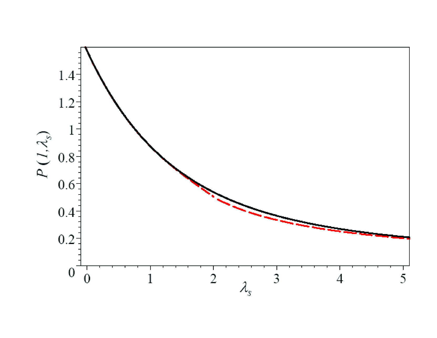
and then divide the result by . The exact calculation of the last integral of (4) yields a function
shown in Fig. 3 by the black solid line. Note that the function is proportional to the average “absorption cross section” [9, Eq. (8e-28)],
| (5) |
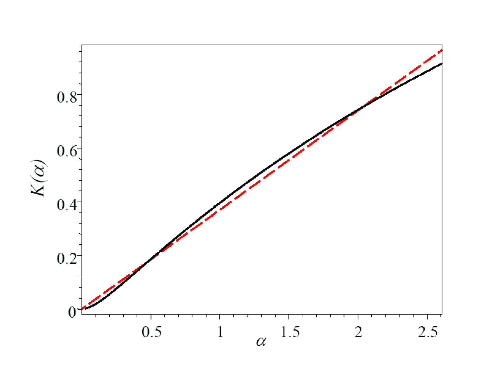
In the energy range of interest, , i.e., , the complex function can be quite accurately approximated by the dependence () shown in Fig. 3 by the red dashed line. This approximation allows us to describe the total average rate of secondary electron production by a simple formula:
| (6) |
where is the photon energy distribution normalized to the total photon density, , and expressed in terms of the full momentum distribution function (Sect. 3) as . Thus, to evaluate the average rate of secondary electron production as a function of the distance from the radiation source, one needs to determine the photon energy distribution along with its distance variations. This requres a collisional kinetic theory for propagating photons.
3 Photon kinetics in spherically symmetric approximation
Radiated and scattered -quanta can be treated as a gas of incoherent and unpolarized photons. For photon energies above 30 keV, this gas is prone mainly to Compton scattering, while at lower energies the photoelectric absorption starts dominating. Both processes result in air molecule ionization, i.e., production of free electrons. The coherent Rayleigh scattering is at least an order of magnitude smaller and can be neglected. Also, the process inverse to photon absorption, viz., photon production during collisions of free electrons with air molecules, in the range of electron energies we are dealing with ( MeV), is negligibly small. Therefore, we will assume the spatial and momentum distribution of photons to be independent of any feedback from the free electrons.
We will treat individual -quanta kinetically as classical particles localized in both real and momentum spaces. The photon momentum distribution, , may have a temporal () and spatial () dependences. Since photons propagate and scatter practically instantaneously we will ingore any temporal dependence. Being concerned mainly with distances from the radioactive material much longer than the container size , we will treat this material as a point-like source of -quanta. Ignoring possible effects of the ground, air inhomogeneity and container anisotropy, we will assume spherically symmetric propagation of photons.
In the spherically symmetric geometry, the photon momentum distribution depends on one spatial variable, viz., the distance of a localized photon from the point-like source, and two momentum components: the absolute value of the momentum, , and the momentum polar angle with respect to the radius vector at the given location, (the latter should not be confused with the angle between the scattered and incident photons, ). Thus the photon momentum distribution is a function of three variables, . Since the angle is not invariant with respect to the collisionless motion, it is more convenient to pass from to the “impact parameter” ,
| (7) |
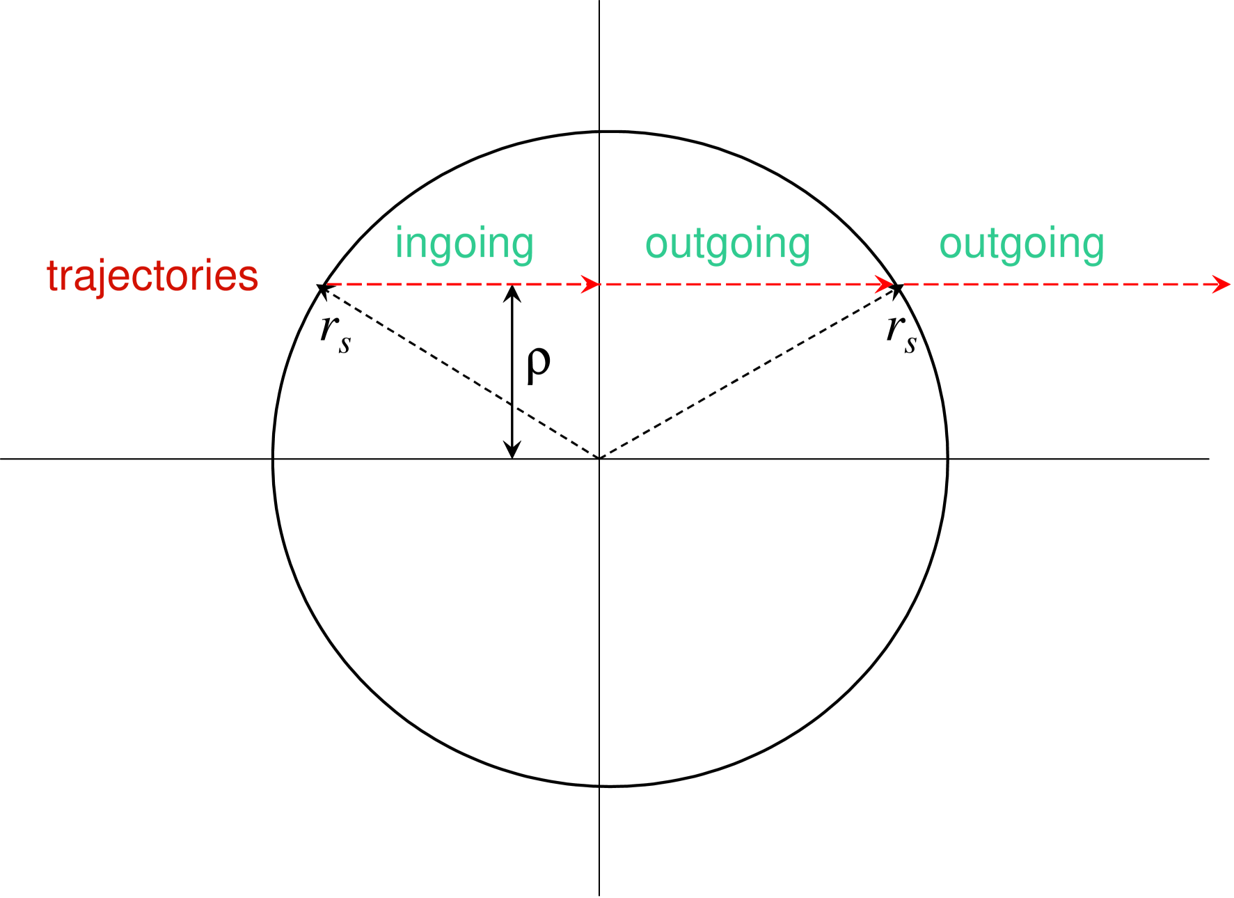
equal to the shortest distance from the radioactive source () to the straight-line trajectory of a freely propagating photon. The parameter is proportional to the photon angular momentum and remains invariant during the free photon propagation. It can be changed only during brief collisions that lead to Compton scattering. For any given positive , we distinguish between two groups of photons with different signs of in (7): the “outgoing” photons with the ‘’ sign (corresponding to ) and “ingoing” photons with the ‘’ sign (), as illustrated by Figure 4. We will denote the two corresponding distribution functions by .
In terms of , the total photon number density, , and radial flux density, , are given by
| (8a) | ||||
| (8b) | ||||
The momentum distribution function of freely propagating -quanta with occasional spiky collisions satisfies the Boltzmann kinetic equation derived in Appendix A,
| (9) |
where the left-hand side describes the collisionless propagation of photons, while the right-hand side (RHS) describes their collisions with air molecules.
The first term in the RHS of (9) describes the kinetic arrival of photons to the elementary phase volume around given due to collisional scattering of incident photons from around ,
| (10) |
where
| (11) | |||
and is the angle of Compton scattering from to ,
| (12) |
(here ). In (10), we keep , for easier integration over the angular variables, but before appplying in the LHS of (9), should be expressed in terms of using (7).
The last term in the RHS of (9) describes the total kinetic departure of -photons due to their scattering with the total collision frequency, , proportional to the total K-N cross-section [4],
| (13) |
Equation (9) should be supplemented by the boundary conditions. In accord with (8b), at a small distance that satisfies , the photon distribution function radiated by the point-like radioactive source can be written as
| (14) |
where is the total number of radioactive decays per unit time, denotes summation over all kinds of primary photons radiated during one disintegration of the radioactive material (usually, ,,) and expresses the fact that all radiated photons have discrete energies (e.g., for Co: , and ). Equation (14) represents the inner boundary condition at applicable to the outgoing photons. For the ingoing photons, we use the natural condition of at . Between consecutive collisions, some ingoing photons pass the minimum distance and become outgoing. This yields the matching condition between the two groups:
| (15) |
Further, all collisional processes lead only to decreasing photon energies, so there are no photons with energies exceeding the initial ones, . Lastly, we assume that at () all momentum distributions behave regularly.
The RHS of (9) satisfies automtically the condition , which provides in accord with (8b) conservation of the total photon flux through any surface surrounding the radiation source. This flux conservation is due to the fact that kinetic equation (9) includes only photon scattering. Photoelectric absorption and other possible photon losses can also be included in by a simple addition to the RHS of (13). Those effects would break the total flux conservation.
Kinetic equation (9) is solved analytically in Appendix B. The complete solution is given by an infinite series of multiply scattered photons (B.2), where is given by (B.1), is determined by recurrence relations (B.4) with the linear integral operator defined by (10). This general solution, however, involves an increasing number of nested integrations which for are difficult to calculate. Below we restrict our treatment to distances from the radiation source located within the mean free path for 1.2 MeV -quanta, (the “near zone”). At these distances, one might expect two dominant photon groups: the primary -quanta beams () and singly scattered photons (). The momentum distribution for singly scattered photons is obtained in Appendix B.2. However, a mere cutoff of the infinite series (B.2) to its first two terms, and given by (B.17)–(B.22), becomes less satisfactory at distances because further scattering of singly scattered photons breaks the total flux conservation. Below we modify the two-group description of photons to make it exactly flux conserving.
4 Photon energy distribution in the near zone
To calculate the total electron production rate given by (6), we need to determine the spatially dependent photon energy distribution at various distances from the radioactive source, , where is the normalized energy. In this section, however, it is more convenient to use
| (16) |
which differs from by the normalization factor following from : . In terms of , (6) becomes
| (17) |
4.1 Primary photons
For the primary photons, we have the solution (B.1) valid for arbitrary distances from the radiation source. The exponential factors there describe the beam attenuation due to Compton scattering. For the corresponding , photon density , total flux and the electron production rate , we obtain simple formulas
| (18) |
4.2 Scattered photons: extended solution
Each primary beam of radiated photons denoted by produces its own set of scattered photons characterized by the corresponding partial distribution function . Bearing in mind that the distribution of all photons is given by and
| (19) |
below we consider separately the partial distributions and the corresponding partial moments.
As a primary beam of photons leaves the radiation source it starts producing scattered photons with the rate, which in the close proximity to the radiation source, , grows linearly with distance. Convolved with the spherical divergence, the population of scattered photons becomes proportional to . Our simulations show that this spatial dependence for the energy distribution of scattered photons roughly holds through the entire near zone, . Until the low-energy photoelectric absorption becomes important, a partial photon flux of all related photons remains constant, . Each partial primary-photon beam decays exponentially due to Compton scattering, , so that at the corresponding flux of scattered photons, , dominates. The corresponding photon density, , where is the mean radial velocity of scattered photons, starts dominating noticeably closer to the radiation source due to the more isotropic momentum distribution () compared to that of the almost perfectly directional primary beam (). The same pertains to the electron production rate, albeit the distance where produced by scattered photons starts dominating at a larger distance than that for the photon density due to the weighting factor in the integrand of (17). (This factor is biased to higher energies where scattered photons momentum distribution is more directional.) Thus electron production due to scattered photons may become important deeply in the near zone, .
We simplify the treatment of scattered photons in the near zone as follows. We will consider all scattered photons, , as one unified group and extend for this group the singly-scattered () photon momentum distribution given by (B.17) and (B.21) with one simple modification. In the exponents of the attenuation factors (B.18) and (B.22), we will retain the terms responsible for the primary beam attenuation, but will ignore . The reason is that the latter terms describe the loss of photons due to their further scattering. For the entire unified group of all scattered photons, this represents just a particle redistribution and hence must be ignored. This will provide automatically the total photon flux conservation.
The extension of the solution to all scattered photons will introduce two inaccuracies. On the one hand, multiply scattered photons decrease their energy as increases, so that photons with leak into the lower-energy range , as discussed in the end of Appendix section B.1. This reduces the photon population in the regular energy range, . Due to the weighting factor in the integrand of (17), this inaccuracy in the extended solution would lead to overestimated . On the other hand, multiply scattered photons have a more isotropic angular distribution in the momentum space that leads to the reduced average photon radial velocity and, hence, to the increased photon density. As a result, the more directional extended solution would, on the contrary, underestimate . We expect the two inaccuracies to partially balance each other. As discussed below by comparing our analytical results with computer simulations, our simplified analytical model describes well the spatial dependence of the photon energy distribution within , practically in the entire near zone (). Thus it can be employed for reliable estimates of the electron production rate in the near zone.
The extended solution is even simpler than the original one because (B.18) and (B.22) reduce to a common attenuation factor, . One can easily check that the modified solution conserves exactly the total photon flux through any closed surface surrounding the radiation source. Indeed, the contributions of the ingoing and outgoing photons at (see Fig. 4) cancel each other. The remaining partial fluxes of the outgoing photons in the outer sphere yield , in full agreement with the flux conservation. Unfortunately, the contributions from the ingoing and outgoing photons within to the photon energy distribution and have no opposite signs and add rather than cancel. This leads to more complicated calculations outlined below.
Using the modified solution, we calculate now the energy distribution of scattered photons. According to the above, the partial momentum distribution assoiciated with a beam is
| (20) |
where
| (21) |
and , introduced in (B.14), describes the distance where the scattering of primary photons took place. Introducing , as in (B.9), we obtain
| (22) |
where the boundary corresponds to () and
| (23a) | ||||
| (23b) | ||||
| The function describes photons scattered forward (). It includes only outgoing photons with (). The function describes photons scattered backward (). In the “inner” zone, (), it includes both ingoing and outgoing photons with equal contributions, while in the “outer” zone, , it includes only outgoing photons. The integrals over describe the original scattering of photons from the primary beams, where the distance of scattering, , depends on the angular parameter and on the photon momenta via . In the near zone, , all outer photons at given were scattered at distances . The situation for the inner photons is different. Some ingoing photons at given could be originally backscattered at large distances, even (for ), well beyond the near zone. The total contribution of these photons, however, should be relatively small due to exponential attenuation of the primary beams described by . Temporarily introducing | ||||
| (24) |
| (25) |
and , we can rewrite the functions and as
| (26) |
The transition from to at corresponding to is smooth. For example, , while is the continuation of the multivalued function from its first quadrant () to the second one (). A similar smooth transition takes place for non-zero .
If then the scatter distances lie within the near zone. However, as mentioned above, ingoing photons scattered backward can arrive from arbitrarily large distances , so we should consider any possible values of . All such photons are described in (26) by the function shown in Fig. 5
and expressed analytically as
| (27) |
where and are the modified Bessel and Struve functions [10]. For a simpler analysis, one can approximate in terms of elementary functions by combining the power series (27) to the fifth-order term with the large- asymptotics, , as
| (28) |
This piece-wise approximation mimics the actual almost ideally except for a minor kink at , as seen in Fig. 5.
Unlike , the function in (26) describes only outgoing photons scattered at distances closer to the source than the given distance . According to the near-zone restriction, , in the entire integration domain of (24), holds. This allows us to expand the exponential function in the integrand of in powers of to the fifth power (applicable for ). This yields
| (29) |
Returning from the temporary notation (25) back to the distance , we obtain
| (30) |
| (31) |
where, according to (27)–(28), the first term in the RHS of (31) can be approximated by elementary functions as
| (34) |
The function describes photons scattered forward (, ), while describes photons scattered backward (, ). The two functions are smoothly connected at (, ). In spite of singular denominators in (30)–(34), and behave regularly at (), except for . At , (, ) approaches , while (, ) increases with decreasing as . This divergence of at is due to accumulation of photons scattered almost strictly backward from distances where the primary beams still remain largely unattenuated, . As increases, even remaining within the mean free path from the radiation source, the exponential attenuation of the primary beams at larger distances makes such accumulation less significant.
Inserting (30) and (31) into (22), with given in terms of by (B.9), i.e.,
| (35) |
we obtain the complete approximate analytical expression for (19) in the near zone.
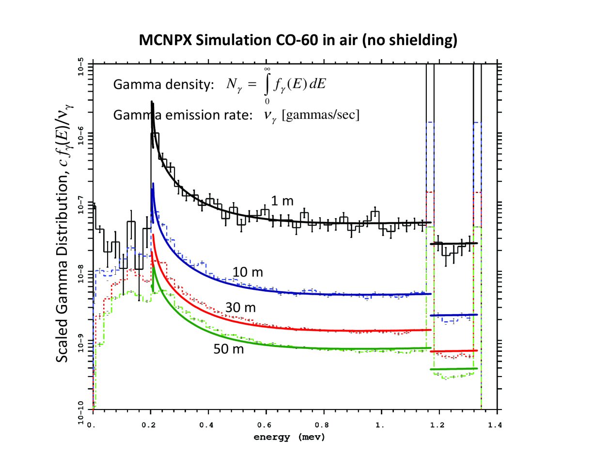
Figure 6 shows photon energy distributions for unshielded Co calculated by the MCNPX code (URL: http://mcnpx.lanl.gov/) and the analytical solution given by (22) and (30)–(35) for several distances (shown near the curves). The two long spikes on the right correspond to the two monochromatic primary photon beams with and MeV, described analytically by (B.1). We see an excellent agreement between the simulations and theory in the entire energy range of singly scattered photons, . At , the simulations show lower-energy multiply scattered photons excluded from the extended model. In the near zone, especially due to the weighting factor in the integrand of (17), the lower-energy range makes a small relative contribution to .
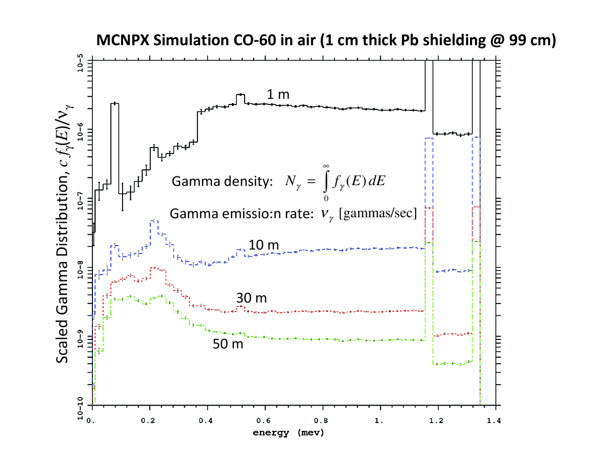
Figure 7 shows simulated photon energy distributions for the same radioactive source but shielded with a thin spherical lead cover. The clearly pronounced broad bumps at the high-energy tails of the photon distribution, especially at the closest proximity to the source () are due to primary photons scattered within the shield material and leaked outside. This scattering could also be described by the general solution (B.1)–(B.4) with defined by (10), where the collisional mean free path for photons in the shielding metal is many orders of magnitude smaller than that in air. Unfortunately, for dense shielding the near-zone approximation is hardly applicable. Besides, photoemission absorption may play a role. This makes analytical calculation much more difficult. Comparing Figs. 6 and 7, we see that the effect of shielding on the energy distribution is especially pronounced in a close proximity to the source. For distances m, the photon energy distribution in both shielded and unshielded cases look similar.
4.3 Electron production rate
Now we calculate the electron production rate (17) due to scattered photons with the energy distribution function given by (22), or
where , and , are given by (30)–(34). We restrict calculations to the radiation material Co with and .
When calclulating the production rate for scattered photons, , it is convenient to compare it with production rate for primary photons given by (18). Straightforward numerical integration shows that for each a simple approximation
| (36) |
holds to a better than 5% accuracy. To compare with , we express , with in terms of by (13), and obtain
As a result, the total electron production rate becomes
| (37) |
where the last term in the RHS brackets represents the ratio between the production rate due to the scattered photons to that due to the primary photons (for each primary beam ) and
| (38) |
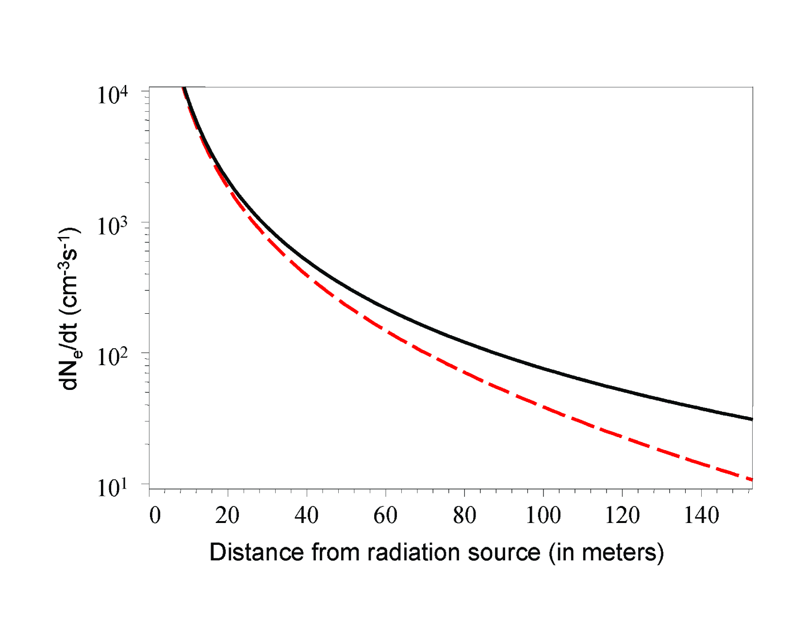
Equation (37) shows that the scattered-photon contribition to the total free-electron production rate decays with distance as , i.e. noticeably slower than that of the primary photons, . For Co, we have , , , and , , . The corresponding is shown in Fig. 8, along with the primary photon rate given by (18). This Figure shows that the latter is a good approximation for . At larger distances, due to scattered photons becomes noticeable and dominates starting from . For simple estimates, we can extrapolate equation (37) to larger distances, but for our application only moderate distances, , matter (see below).
Figure 8 also shows that a moderate amount () of a concealed radioactive material like Co can provide the total rate of electron production well above the background level ( pairs ). The enhancement factor exceeds unity within from the radiation source. This distance is crucial for implementation of our technique because … As discussed in Ref. [3], all free electrons will eventually end up forming negative ions, but the collisional detachment of some electrons for a brief time make it sufficient to initiate air breakdown within the focal spot of the THz gyrotron during pulse. Equation (37) provides a reliable estimate of the electron production rate at least within the distance of critical for implementation of our method.
Conclusion:
In this paper, we analyze the production of free electrons by -rays leaking from radioactive materials. This is important for implementation of a recently proposed concept to remotely detect concealed radioactive materials [1], [3]. We have performed our analysis specifically for the most probable radioactive material Co, but the general approach can be applied to any -ray sources. In our theory, we have included free-electron production by both primary -quanta radiated by the source and penetrated through the container walls and those scattered in air. Equation (37) and Fig. 8 give a reliable estimate of the total production rate and the corresponding radiation enhancement factor, at least within from the radiation source. At these distances, the scattered photon contribution to is comparable or even exceeds that of the primary photons. Even for amount of radiation material as small as , the total production rate may exceed significantly the ambient ionization rate. During the gyrotron pulse of about 10 microsecond length, such electrons may seed the electric breakdown and create sufficiently dense plasma at the focal region to be detected as an unambiguous effect of the concealed radioactive material.
Acknowledgement:
This work is supported by the US Office of Naval Research.
Appendix
Appendix A Deriving kinetic equation (9)
The Boltzmann kinetic equation for freely propagating unpolarized photons colliding with air molecules contains two parts: the collisionless part describing the undisturbed propagation of photons between two consecutive acts of scattering or absorption and the collisional operator [8]. In the assumed spherically symmetric approximation, the stationary kinetic equation for with given by (7) can be written as
| (A.1) |
The LHS of (A.1) contains no -derivatives because these variables are invariants of the collisionless motion. The collisional term describes scattering, absorption and other possible effects responsible for collisional changes in the photon momentum distribution. In the general case, it has a complicated integral form which can be simplified in the spherically symmetric case.
In this appendix, we obtain the explicit simplified form for . We will start directly from the original probabilistic expressions like [8]. Since the photon-molecule collision is a strictly local process where the photon transport plays no role, in the RHS of (A.1) we can temporarily return from back to the momentum polar angle .
| (A.2) | ||||
Here describes the total collisional departure of photons from the kinetic volume around given with scattered photon momenta in the domain and releasing electrons in around and , respectively. In the general case, the departure term, , can include both photon scattering and absorption. The term describes the arrival of photons and released electrons into the volumes and around and , respectively, if the incident photons before scattering were at around . Since we neglect any collisional photon production like Bremsstrahlung, fluorescence, etc., includes only photon scattering. With no photon losses included in , (A.2) provides automatically the particle conservation, .
The function of two arguments and represents the probability per unit time of the collisional process. This function is proportional to the air molecular density, . In the general case, the two arguments of are not interchangeable. To identify the correct order of the arguments, the time sequence of the collision is denoted by the arrow. The two delta-functions in the integrands describe the energy and momentum conservation. Since we assume energies well above the K-shell edge, the arguments of the delta functions include no small energy spent on the molecule excitation and ionization. They also neglect the kinetic energy and momentum of air molecules. As explained in section 3, we presume Compton scattering in the K-N approximation.
To obtain the explicit expression for , we relate it to the corresponding differential collision cross section, , given for the K-N theory by Eq. (2). To find the expression is easier through the departure term because, unlike , it does not involve the photon distribution function in the integrand. Integrating (A.2), first, over with eliminating and then over in with eliminating the remaining delta-function, we obtain
| (A.3) |
Here is the total density of bound electrons and should be calculated from the momentum conservation, , but before applying the energy conservation, . As a result, we arrive at
| (A.4) |
where is the scatter angle from to given by (3). This results in , where is given by (13).
Now we proceed to calculating the more complicated arrival term, . Switching in (A.4) the arguments of , we obtain
| (A.5) |
where in terms of and is given by (12). After inserting (A.5) to (A.2), as above, the first step to calculating is to integrate over with eliminating . This yields
| (A.6) |
Unlike , however, the arrival term contains the distribution function within the integrand. This does not allow us to easily integrate over in in order to eliminate the remaining delta function. However, the fact that the distribution function depends on and , rather than on the axial angle suggests eliminating the remaining delta function via the integration over , using a simple geometric relation
| (A.7) |
Given , this yields . Integration of in (A.2) over using
| (A.8) |
results in
| (A.9) |
The factor in (A.9) originates from existence of two symmetric values of that set the argument of the delta-function to zero (the energy conservation)
| (A.10) |
The specific value of in (A.8) is inconsequential. The differentiation in the normalization factor should be done using (A.6) and (A.7), but before applying (A.10). This yields . Using (A.7) again in order to express and then, applying the energy conservation relation (A.10), we obtain , where
| (A.11) |
Implementing the entire procedure, we arrive at the integro-differential equation (9), where is recast as (11). This fully symmetric function of three cosine arguments has a simple physical meaning. The restriction covers all possible directions of the incident and scattered photons characterized by the pairs of polar and axial angles , , , which are coupled by geometric relations like (A.7). The photon energy losses and the scattering angle are rigidly coupled by (12). A photon with given , can be scattered into another photon with given , , provided the photon energies are within the allowed domains. This freedom is reached by a unique choice of two symmetric values of .
Appendix B Solving kinetic equation (9)
B.1 General solution of multi-scattered photons
The LHS of kinetic equation (9) is simple, but its RHS is rather complicated, as described by (10). Our approach to solving the kinetic equation is based on the physics of the process. The primary photons with the monochromatic momentum distribution approximated by (14) start efficiently scattering by air molecules within a distance of from the source. For photon energies between and , the maximum K-N differential cross-section is reached near the forward scattering, and gradually decreases to the backscatter, , as shown in Fig. 2. This means that photons scatter mainly through large angles, rather than broaden their delta-function angular distribution around the primary beam. This suggests considering the primary photon beam as a separate group that continues keeping its delta-function distribution over long distances from the radiation source. For the primary photons, we can neglect the first (“arrival”) term in the RHS of (9) but must keep the last (“departure”) term. Using the boundary condition (14), we readily obtain for the primary photons the exponentially decaying solution,
| (B.1) |
This solution gives the entire local source for scattered photons. The solution for all propagating photons, including the primary beam, can be sought as an infinite series
| (B.2) |
where and the subscript denotes photons scattered from the primary beam times. For each individual group of -scattered photons, we obtain a recursive kinetic equation where the source for scattering is provided by the -th group,
| (B.3) |
where is the linear integral operator defined by (10). The infinite series given by (B.2) converges. If includes no absorption then Eq. (B.3) provides automatically the constancy of the total photon flux through any closed surface surrounding the radiation source. Using the boundary and matching conditions for the outgoing () and ingoing () particles described above, we obtain the exact recursive solution for in terms of , ,
| (B.4) | ||||
This solution holds for , while for all . As mentioned above, the integrations for in (10) can be performed it terms of , but before inserting the results to (B.4) they have to be transformed into functions of using (7). In the integrands of (B.4), the distance is replaced by an internal radial variable in order to avoid a confusion with outside the integral. The exponential factors describe -photon losses due to their scattering into the -group with describing the distance between two points on the - and -shells along a straight-line photon trajectory corresponding to given (the signs depend on whether the two points are on the same or on different sides with respect to the trajectory median , as shown in Fig. 4). The summations over the ingoing and outgoing particles in (B.4) take into account the fact that photons can be scattered through arbitrary scatter angles, so that any ingoing or outgoing particle can be scattered into each of these groups.
The explicit solution for scattered photons with arbitrarily large can be found by consecutively applying recursive relation (B.4) starting from with given by Eq. (B.1). At any given distance , photons with sufficiently large are produced mainly by ingoing photons that originate from the primary source beam at much larger distances and only accidentally come back. One might expect that they will come back less frequently as increases, so that the infinite series (B.2) will converge. Additionally, as increases, the photon energy distribution gradually moves to lower energies. This effective ”cooling” of scattered photons will eventually put high- scattered photons into the keV range where the photoemission absorption of photons starts dominating.
We can easily estimate the energy spread for times scattered photons. The maximum energy of scattered photons, , where is the ionization potential, , is reached where is close to , but not too close [4, Sect. 2.6.2.1]. As a result, after scatterings of a primary -quanta with , the maximum scattered photon energy reduces only weakly, , while in the framework of the K-N theory . On the other hand, the minimum energy of scattered photons is reached for strict backscatter, [4]. After scatterings, the minimum energy, , decreases by the following rule,
| (B.5) |
starting from . Temporarily denoting , we obtain from (B.5) , so that , or
| (B.6) |
The energy of -times scattered photons spreads between and . This spread gradually increases with due to lowering . For , , so that after 2–3 scatterings the minimum photon energy becomes almost inversely proportional to , . Hence, after scatterings, the minimum energy falls well into the range where photoemission absorption starts dominating. This low-energy photon absorption creates an effective sink for multiply scattered photons.
B.2 Solution for
Here we consider the lowest-order scattered photons, . In the relatively near zone, , the cutoff of the infinite chain by the first term of the series represents a good approximation for the entire photon distribution.
For , we obtain from (B.4),
| (B.7) | ||||
Here is given by
| (B.8) |
where is given by (12) and, accordingly,
| (B.9) |
| (B.10) |
In accord with (B.1), we obtain
| (B.11) |
Unlike general equation (B.4), (B.7) contains no summations over because the primary photon beams include no ingoing photons. Integration in (B.8) over should be done with care because the straightforward elimination of () with leads to a singularity. To avoid it, we apply the following. Regardless of the specific values of and , the integral equals , so that we obtain
| (B.12) |
and hence
| (B.13a) | ||||
| where , | ||||
| (B.14) |
These expressions have a simple physical meaning. Photons from the radiated monochromatic and infinitely narrow beams are scattered into angles rigidly coupled to the energy of the scattered photon. Given both the energy and of the scattered photon, one can find the distance where such act of scattering took place, . The delta-function demonstrates the uniqueness of this scattering distance. The factor describes the total attenuation of the primary beam on its way from the radiation source to .
Now we insert the expression for into (B.7), integrate with eliminating and use relation (B.14): , . The result depends upon whether the photon momentum is less or greater than a critical value, , corresponding to the -scattering () from the primary beam . For
| (B.15) |
all singly-scattered particles are outgoing particles caused by forward scattering (), while for scattered particles are either ingoing or outgoing particles caused by backscatter ().
Depending on whether or , we will separate between ‘outer’ and ‘inner’ photons. For , all scattered photons are outer () outgoing photons,
| (B.16) |
originating from only one scattering location with given . We have then
| (B.17) |
where the attenuation factor is
| (B.18) |
For , or more precisely, for
| (B.19) |
there are both outer outgoing and inner () photons,
| (B.20) |
either outgoing or ingoing from two different locations of given . For the outer photons defined by (B.16), we have the same solution as (B.17). For the inner photons, we have two solutions for the either ingoing or outgoing photons,
| (B.21) |
which differ by the attenuation factors only,
| (B.22) |
There are different signs in front of due to the fact that for the outgoing photons the two points corresponding to and lie on the two opposite sides from , so that the two distances and add, rather than subtract, as they do for the ingoing photons.
Note that the only -dependence in the above distributions is due to the attenuation factors. As functions of the angular variable , contains only a singular factor . Since all integrals for calculating the photon densities and fluxes contain this singularity is integrable.
References
- [1] V. L. Granatstein and G. S. Nusinovich, J. Appl. Phys., 108, 063304 (2010).
- [2] G. S. Nusinovich et al., J. Infrared, Millimeter, Terahertz Waves, 32, 380 (2011)
- [3] G. S. Nusinovich, P. Sprangle, C. A. Romero-Talamas and V. L. Granatstein, J. Appl. Phys., 109, 083303 (2011).
- [4] N. J. Carron, “An Introduction to the Passage of Energetic Particles through Matter,” Taylor & Francis, New York, 2001.
- [5] G. F. Knoll, “Radiation detection and measurement,” 3rd Edition, Wiley, New York, 2000.
- [6] W. P. Jesse and J. Sadauskis, Phys. Rev. 97, 1668 (1955).
- [7] J. M. Valentine and S. C Curran, Rep. Progr. in Physics, 21, 1-29 (1958).
- [8] E. M. Lifshitz and L. P. Pitaevskii, “Physical Kinetics” (“Course of Theoretical Physics”, Volume 10), Butterworth-Heinemann, Oxford, UK, 2002.
- [9] D. E. Gray (Coord. Ed.), American Institute of Physics Handbook, Third Ed., McGraw-Hill, New York, 1972.
- [10] M. Abramowitz and I. A. Stegun, Handbook of Mathematical Functions: with Formulas, Graphs and Mathematical Tables, Dover Publications, 1999.