Propagation time for zero forcing on a graph
Abstract
Zero forcing (also called graph infection) on a simple, undirected graph is based on the color-change rule: If each vertex of is colored either white or black, and vertex is a black vertex with only one white neighbor , then change the color of to black. A minimum zero forcing set is a set of black vertices of minimum cardinality that can color the entire graph black using the color change rule. The propagation time of a zero forcing set of graph is the minimum number of steps that it takes to force all the vertices of black, starting with the vertices in black and performing independent forces simultaneously. The minimum and maximum propagation times of a graph are taken over all minimum zero forcing sets of the graph. It is shown that a connected graph of order at least two has more than one minimum zero forcing set realizing minimum propagation time. Graphs having extreme minimum propagation times , , and are characterized, and results regarding graphs having minimum propagation time are established. It is shown that the diameter is an upper bound for maximum propagation time for a tree, but in general propagation time and diameter of a graph are not comparable.
Keywords zero forcing number, propagation time, graph
AMS subject classification 05C50, 05C12, 05C15, 05C57, 81Q93, 82B20, 82C20
1 Propagation time
All graphs are simple, finite, and undirected. In a graph where some vertices are colored black and the remaining vertices are colored white, the color change rule is: If is black and is the only white neighbor of , then change the color of to black; if we apply the color change rule to to change the color of , we say forces and write (note that there may be a choice involved, since as we record forces, only one vertex actually forces , but more than one may be able to). Given an initial set of black vertices, the final coloring of is the set of black vertices that results from applying the color change rule until no more changes are possible. For a given graph and set of vertices , the final coloring is unique [1]. A zero forcing set is an initial set of vertices such that the final coloring of is . A minimum zero forcing set of a graph is a zero forcing set of of minimum cardinality, and the zero forcing number, denoted , is the cardinality of a minimum zero forcing set.
Zero forcing, also known as graph infection or graph propagation, was introduced independently in [1] for study of minimum rank problems in combinatorial matrix theory, and in [3] for study of control of quantum systems. Propagation time of a zero forcing set, which describes the number of steps needed to fully color a graph performing independent forces simultaneously, was implicit in [3] and explicit in [8]. Recently Chilakamarri et al. [4] determined the propagation time, which they call the iteration index, for a number of families of graphs including Cartesian products and various grid graphs. Control of an entire network by sequential operations on a subset of particles is valuable [8] and the number of steps needed to obtain this control (propagation time) is a significant part of the process. In this paper we systematically study propagation time.
Definition 1.1.
Let be a graph and a zero forcing set of . Define , and for , is the set of vertices for which there exists a vertex such that is the only neighbor of not in . The propagation time of in , denoted , is the smallest integer such that .
Two minimum zero forcing sets of the same graph may have different propagation times, as the following example illustrates.
Example 1.2.
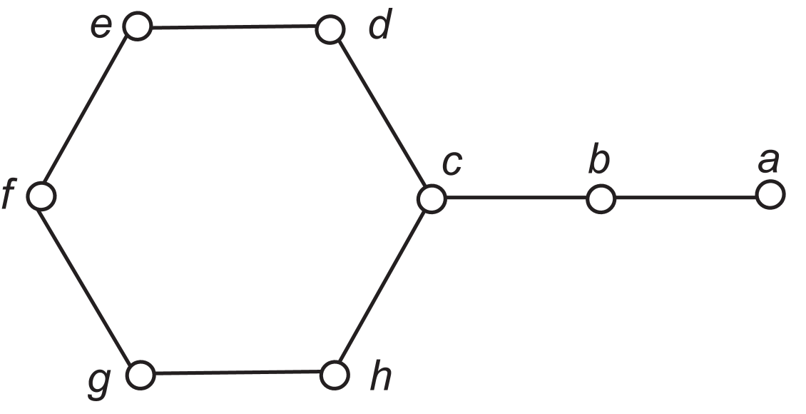
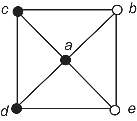
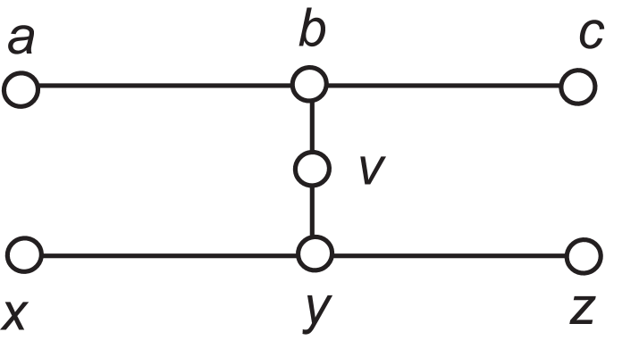
Let be the graph in Figure 1. Let and . Then , , , , and , so . However, , , , and , so .
Definition 1.3.
The minimum propagation time of is
Definition 1.4.
Two minimum zero forcing sets and of a graph are isomorphic if there is a graph automorphism of such that .
It is obvious that isomorphic zero forcing sets have the same propagation time, but a graph may have non-isomorphic minimum zero forcing sets and have the property that all minimum zero forcing sets have the same propagation time.
Example 1.5.
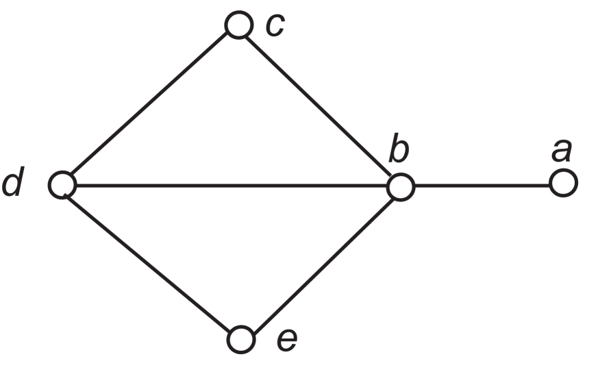
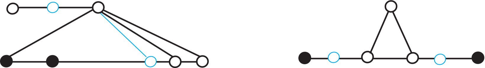
Up to isomorphism, the minimum zero forcing sets of the dart shown in Figure 2 are , and . Each of these sets has propagation time .
The minimum propagation time of a graph is not subgraph monotone. For example, it is easy to see that the 4-cycle has and . By deleting one edge of , it becomes a path , which has and .
A minimum zero forcing set that achieves minimum propagation time plays a central role in our study, and we name such a set.
Definition 1.6.
A subset of vertices of is an efficient zero forcing set for if is a minimum zero forcing set of and . Define
We can also consider maximum propagation time.
Definition 1.7.
The maximum propagation time of is defined as
The bounds in the next remark were also observed in [4].
Remark 1.8.
Let be a graph. Then
because at least one force must be performed at each time step, and
because using a given zero forcing set , at most forces can be performed at any one time step.
Definition 1.9.
The propagation time interval of is defined as
The propagation time discrepancy of is defined as
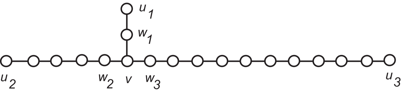
It is not the case that every integer in the propagation time interval is the propagation time of a minimum zero forcing set; this can be seen in the next example. Let be the generalized star with three arms having vertices with ; is shown in Figure 3.
Example 1.10.
Consider with . The vertices of degree one are denoted by , the vertex of degree three is denoted by , and neighbors of are denoted by . The minimum zero forcing sets and their propagation times are shown in Table 1. Observe that the propagation time interval of is , but there is no minimum zero forcing set with propagation time . The propagation discrepancy is .
The next remark provides a necessary condition for a graph to have .
Remark 1.11.
Let be a graph. Then every minimum zero forcing set of is an efficient zero forcing set if and only if . In [2], it is proven that the intersection of all minimum zero forcing sets is the empty set. Hence, implies .
In Section 2 we establish properties of efficient zero forcing sets, including that no connected graph of order more than one has a unique efficient zero forcing set. In Section 3 we characterize graphs having extreme propagation time. In Section 4 we examine the relationship between propagation time and diameter.
2 Efficient zero forcing sets
In [2] it was shown that for a connected graph of order at least two, there must be more than one minimum zero forcing set and furthermore, no vertex is in every minimum zero forcing set. This raises the questions of whether the analogous properties are true for efficient zero forcing sets (Questions 2.1 and 2.14 below).
Question 2.1.
Is there a connected graph of order at least two that has a unique efficient zero forcing set?
We show that the answer to Question 2.1 is negative. First we need some terminology. For a given zero forcing set of , construct the final coloring, listing the forces in the order in which they were performed. This list is a chronological list of forces of [6]. Many definitions and results concerning lists of forces that have appeared in the literature involve chronological (ordered) lists of forces. For the study of propagation time, the order of forces is often dictated by performing a force as soon as possible (propagating). Thus unordered sets of forces are more useful than ordered lists when studying propagation time, and we extend terminology from chronological lists of forces to sets of forces.
Definition 2.2.
Let be a graph, a zero forcing set of . The unordered set of forces in a chronological list of forces of is called a set of forces of .
Observe that if is a zero forcing set and is a set of forces of , then the cardinality of is . The ideas of terminus and reverse set of forces, introduced in [2] for a chronological list of forces and defined below for a set of forces, are used to answer Question 2.1 negatively (by constructing the terminus of a set of forces of an efficient zero forcing set).
Definition 2.3.
Let be a graph, let be a zero forcing set of , and let be a set of forces of . The terminus of , denoted , is the set of vertices that do not perform a force in . The reverse set of forces of , denoted here as , is the result of reversing each force in . A forcing chain of is a sequence of vertices such that for , forces in ( is permitted). A maximal forcing chain is a forcing chain that is not a proper subset of another forcing chain.
The name “terminus” reflects the fact that a vertex does not perform a force in if and only if it is the end point of a maximal forcing chain (the latter is the definition used in [2], where such a set is called a reversal of ). In [2], it is shown that if is a zero forcing set of and is a chronological list of forces, then the terminus of is also a zero forcing set of , with the reverse chronological list of forces (to construct a reverse chronological list of forces of , write the chronological list of forces in reverse order and reverse each force in ).
Observation 2.4.
Let be a graph, a minimum zero forcing set of , and a set of forces of . Then is a set of forces of and .
When studying propagation time, it is natural to examine sets of forces that achieve minimum propagation time.
Definition 2.5.
Let be a graph and a zero forcing set of . For a set of forces of , define and for , is the set of vertices such that the force appears in , , and is the only neighbor of not in . The propagation time of in , denoted , is the least such that .
Let be a graph, let be a zero forcing set of , and let be a set of forces of . Clearly, for all .
Definition 2.6.
Let be a graph and let be a zero forcing set of . A set of forces is efficient if . Define
If is an efficient set of forces of a minimum zero forcing set of , then is necessarily an efficient zero forcing set. However, not every efficient set of forces conforms to the propagation process.
Example 2.7.
Let be the graph in Figure 4. Since every degree one vertex must be an endpoint of a maximal forcing chain and since is a zero forcing set, . Since or must be a maximal forcing chain for any set of forces of a minimum zero forcing set, . Then is an efficient zero forcing set with efficient set of forces Observe that (i.e., does not turn black until step in ), but ( can be forced by at step ).
Definition 2.8.
Let be a graph, a zero forcing set of , and a set of forces of . Define and for , define
Observe that .
Lemma 2.9.
Let be a graph, a zero forcing set of , and a set of forces of . Then .
Proof.
Recall that is a set of forces of . The result is established by induction on . Initially, . Assume that for , . Let . In , at time . In , cannot perform a force until time or later, so . If then in cannot perform a force before time , so . So if , then . Thus . ∎
Corollary 2.10.
Let be a graph, a minimum zero forcing set of , and a set of forces of . Then
Theorem 2.11.
Let be a graph, an efficient zero forcing set of , and an efficient set of forces of . Then is an efficient set of forces and is an efficient zero forcing set. Every efficient zero forcing set is the terminus of an efficient set of forces of an efficient zero forcing set.
The next result answers Question 2.1 negatively.
Theorem 2.12.
Let be a connected graph of order greater than one. Then .
Proof.
Let and let be an efficient set of forces of . By Theorem 2.11, . Since is a connected graph of order greater than one, . ∎
We now consider the intersection of efficient zero forcing sets. The next result is immediate from Theorem 2.11.
Corollary 2.13.
Let be a graph. Then .
Question 2.14.
Is there a connected graph of order at least two and a vertex such that is in every efficient zero forcing set?
The next example provides an affirmative answer.
Example 2.15.
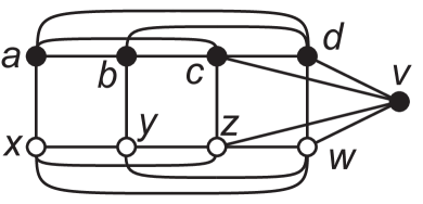
The wheel is the graph shown in Figure 5. The efficient zero forcing set of shows that . Up to isomorphism, there are two types of minimum zero forcing sets in . One set contains and two other vertices that are adjacent to each other; the other contains three vertices other than . The latter is not an efficient zero forcing set of , because its propagation time is . The possible choices for an efficient zero forcing set are or . Therefore, .
We examine the effect of a nonforcing vertex in an efficient zero forcing set. This result will be used in Section 3.2. It was shown in [5] that if and only if there exists a minimum zero forcing set containing and set of forces in which does not perform a force. The proof of the next proposition is the same but with consideration restricted to an efficient zero forcing set (the idea is that the same set of forces works for both and , with included in the zero forcing set for ).
Proposition 2.16.
For a vertex of a graph , there exists an efficient zero forcing set containing and an efficient set of forces in which does not perform a force if and only if and .
3 Graphs with extreme minimum propagation time
For any graph , it is clear that In this section we consider the extreme values , , i.e., high propagation time, and, and , i.e., low propagation time.
3.1 High propagation time
The case of propagation time is straightforward, using the well known fact [7] that if and only if is a path.
Proposition 3.1.
For a graph , the following are equivalent.
-
1.
.
-
2.
.
-
3.
.
-
4.
is a path.
We now consider graphs that have maximum or minimum propagation time equal to .
Observation 3.2.
For a graph ,
-
1.
implies , but not conversely (see Lemma 3.4 for an example).
-
2.
if and only if and exactly one force is performed at each time for every minimum zero forcing set.
-
3.
if and only if and there exists a minimum zero forcing set such that exactly one force performed at each time.
Lemma 3.3.
Let be a disconnected graph. Then the following are equivalent.
-
1.
.
-
2.
.
-
3.
.
Proof.
Clearly . So assume . Since , has exactly two components. At least one component of is an isolated vertex (otherwise, more than one force occurs at time step one), and so . ∎
A path cover of a graph is a set of vertex disjoint induced paths that cover all the vertices of , and the path cover number is the minimum number of paths in a path cover of . It is known [6] that for a given zero forcing set and set of forces, the set of maximal zero forcing chains forms a path cover and thus
A graph is a graph on two parallel paths if can be partitioned into disjoint subsets and so that the induced subgraphs are paths, can be drawn in the plane with the paths and as parallel line segments, and edges between the two paths (drawn as line segments, not curves) do not cross; such a drawing is called a standard drawing. The paths and are called the parallel paths (for this representation of as a graph on two parallel paths).
Let be a graph on two parallel paths and . If , then denotes the parallel path that contains and denotes the other of the parallel paths. Fix an ordering of the vertices in each of and that is increasing in the same direction for both paths in a standard drawing. With this ordering, let and denote the first and last vertices of . If , then means precedes in the order on . Furthermore, if and , is the neighbor of in such that ; is defined analogously (for ).
Row [7] has shown that if and only if is a graph on two parallel paths. Observe that for any graph having , a set of forces of a minimum zero forcing set naturally produces a representation of as a graph on two parallel paths with the parallel paths being the maximal forcing chains. The ordering of the vertices in the parallel paths is the forcing order.
Lemma 3.4.
For a tree , if and only if (sometimes called a T-shaped tree). The graph is the only tree for which .
Proof.
It is clear that , and .
Suppose first that is a tree such that . Then is a graph on two parallel paths and . There is exactly one edge between the two paths. Observe that must have an endpoint not in , so without loss of generality and neither nor is an endpoint of . If is a graph with multiple vertices in each of (i.e., if ), then no matter which minimum zero forcing set we choose, more than one force will occur at some time. So assume consists of a single vertex . If the parallel paths were constructed from a minimum zero forcing set , then , and without loss of generality . If , then at time one, two vertices would be forced. Thus and .
Now suppose that is a tree such that . This implies , so . Since implies , . ∎
Observation 3.5.
If is one of the graphs shown in Figure 6, then , because the black vertices are a minimum zero forcing set with .
For any graph and vertices , denotes that and are adjacent, and denotes the edge with endpoints and .
Definition 3.6.
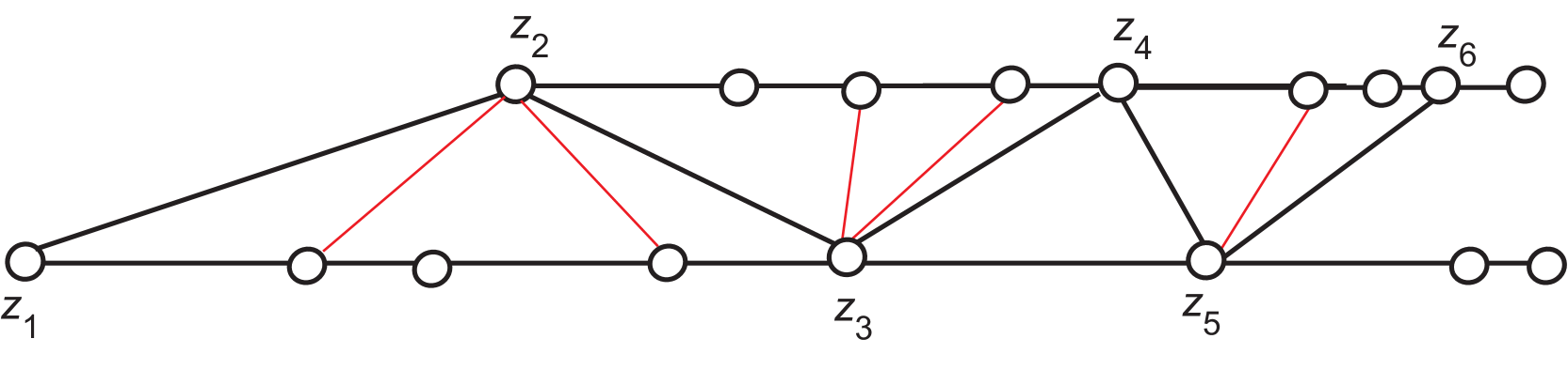
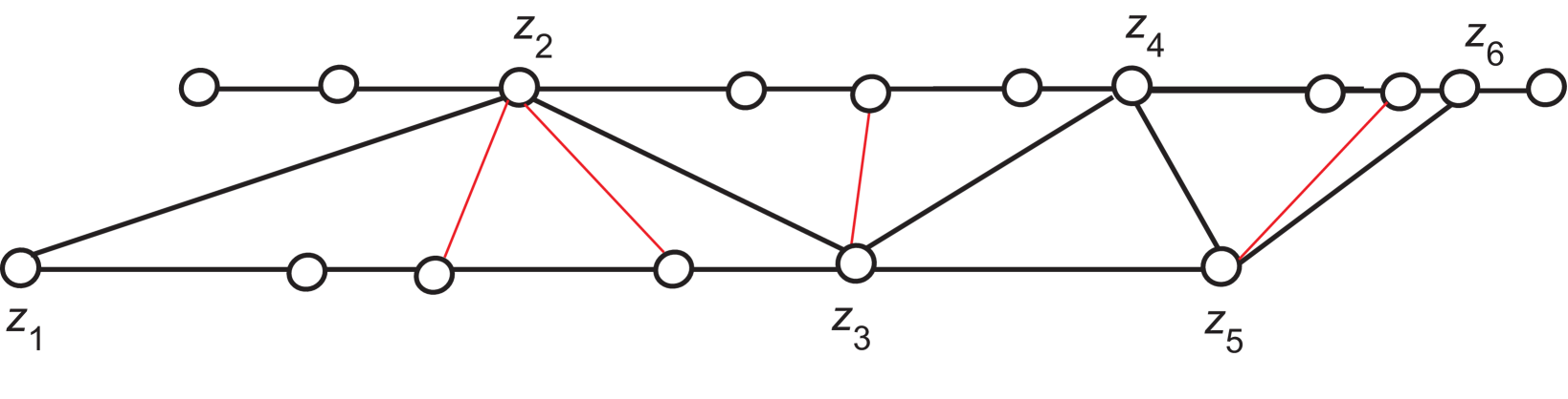
A graph on two parallel paths and is a zigzag graph if it satisfies the following conditions:
-
1.
There is a path that alternates between the two paths and such that:
-
(a)
and for ;
-
(b)
for .
-
(a)
-
2.
Every edge of is an edge of one of , or , or is an edge of the form
The number of vertices in is called the zigzag order.
Theorem 3.7.
Let be a graph. Then if and only if is one of the following:
-
1.
.
-
2.
.
-
3.
A zigzag graph of zigzag order such that all of the following conditions are satisfied:
-
(a)
is not isomorphic to one of the graphs shown in Figure 6.
-
(b)
or (both paths cannot begin with degree-one vertices).
-
(c)
or (both paths cannot end with degree-one vertices).
-
(d)
or
-
(e)
or
-
(a)
Proof.
Assume . If is disconnected or a tree, then is or by Lemmas 3.3 and 3.4. So assume is connected and has a cycle.
First we identify and for : By Observation 3.2, there exists a minimum zero forcing set of cardinality 2 such that exactly one force is performed at each time for . Renumber the vertices of as follows: vertices , zero forcing set with , and vertex is forced at time . Then is a graph on two parallel paths and , which are the two maximal forcing chains (with the path order being the forcing order). Observe that and , because can immediately force and cannot. If and , then choose to be , and let . Otherwise, choose to be and let . For , define until . Define . With this labeling, is a zigzag graph.
Now we show that satisfies conditions (3a) – (3e). Since , is not isomorphic to one of the graphs shown in Figure 6, i.e., condition (3a) is satisfied. Since is the first vertex in one of the paths and , condition (3b) is satisfied. The remaining conditions must be satisfied or there is a different zero forcing set of two vertices with lower propagation time: if (3c) fails, use ; if (3d) fails, then and , so use ; if (3e) fails, this is analogous to (3d) failing, so use .
For the converse, for or by Lemmas 3.3 and 3.4. So assume is a zigzag graph satisfying conditions (3a) – (3e). The sets and are minimum zero forcing sets of , and for . If , so , then is a zero forcing set and . If , so , then is a zero forcing set and . If is not isomorphic to one of the graphs shown in Figure 6, these are the only minimum zero forcing sets. ∎
3.2 Low propagation time
Observation 3.8.
For a graph , the following are equivalent.
-
1.
.
-
2.
.
-
3.
.
-
4.
has no edges.
Next we consider . From Remark 1.8 we see that if , then . The converse of this statement is false:
Example 3.9.
Let be the graph obtained from by appending a leaf to one vertex. Then and .
Theorem 3.10.
Let be a connected graph such that . For , if and only if for every , .
Proof.
If for every , , then cannot perform a force in an efficient set of forces, so for every . Thus .
Now suppose and let . If performs a force in an efficient set of forces of , then . By Theorem 2.11, , so cannot perform a force in any such . Since cannot perform a force, . It is shown in [2] that (assuming the graph is connected and of order greater than one) every vertex of a minimum zero forcing set must have a neighbor not in the zero forcing set. Since , , and so . ∎
We now consider the case of a graph that has and . Examples of such graphs include the hypercubes [1].
Definition 3.11.
Suppose and are graphs of equal order and is a bijection. Define the matching graph to be the graph constructed as the disjoint union of and the perfect matching between and defined by .
Matching graphs play a central role in the study of graphs that have propagation time one.
Proposition 3.12.
Let be a graph. Then any two of the following conditions imply the third.
-
1.
.
-
2.
.
-
3.
is a matching graph
Proof.
: Let be an efficient zero forcing set of and let . Since and , every element must perform a force at time one. Thus and there exists a perfect matching between and defined by where . Then .
For the remaining two parts, assume and ().
: Since , is a minimum zero forcing set and .
: Since , , and because is a zero forcing set with . ∎
We examine conditions that ensure and thus . The choice of matching affects the zero forcing number and propagation time, as the next two examples show.
Example 3.13.
The Cartesian product is , where is the identity mapping. It is known [1] that and thus .
Example 3.14.
The Petersen graph can be constructed as where . It is known [1] that and thus .
Let denote the number of components of .
Theorem 3.15.
Let and let be a bijection. If , then .
Proof.
Assume it is not the case that . This implies is not the union of perfect matchings between the components of and the components of . Without loss of generality, there is a component of that is not matched within a single component of . Then there exist vertices and in such that , , and and are separate components of . We show that there is a zero forcing set of size for , and thus pt. Let , , and , so . Then 1) for , 2) , 3) for , and 4) for all in the remaining components of . Therefore B is a zero forcing set, , and thus . ∎
Theorem 3.16.
Let and let be a bijection of vertices of and (with acting on the vertices of ). Then if and only if is connected.
Proof.
If is not connected, then by Theorem 3.15. Now assume is connected and let . Let with . We show is not a zero forcing set. This implies and thus . Let and . For , cannot perform a force until at least vertices in are black. If then no force can be performed. So assume . Until at least vertices in are black, all forces must be performed by vertices in . We show that no more than vertices in can turn black. Perform all forces of the type with . For each such force, must be black already. Thus at most such forces within can be performed. So there are now at most black vertices in . Note first that if at most vertices of are black, then after all possible forces from to are done, no further forces are possible, and at most vertices in are black. So assume vertices of are black. Let be white. Since is connected, there must be a neighbor of in , and is black. Since and is white, has not performed a force. If were black, there would be at most black vertices in , so is white. After preforming all possible forces from to , at most vertices in are black because all originally black vertices have black, there are black vertices in , and cannot perform a force at this time (since both and are white). Thus not more than vertices of can be forced, and is not a zero forcing set. ∎
The Cartesian product of with is one way of constructing matching graphs, because . Examples of graphs having include the complete graph and hypercube [1]. Since [1], to have it is necessary that , but that condition is not sufficient.
Example 3.17.
Observe that for . But , so .
The next theorem provides conditions that ensure that iterating the Cartesian product with gives a graph with propagation time one. Recall that one of the original motivations for defining the zero forcing number was to bound maximum nullity, and the interplay between these two parameters is central to the proof of the next theorem. Let be a graph. The set of symmetric matrices described by is The maximum nullity of is It is well known [1] that . The next theorem provides conditions that are sufficient to iterate the construction of taking the Cartesian product of a graph and and obtain minimum propagation time equal to one.
Theorem 3.18.
Suppose is a graph with and there exists a matrix such that . Then
Furthermore, for
and .
Proof.
Given the matrix , define
Then and . Since , . Therefore, . Then
so we have equality throughout. Since is a matching graph, by Proposition 3.12. ∎
Let denote the graph constructed by starting with and performing the Cartesian product with times. For example, the hypercube , and the proof given in [1] that is the same as the proof of Theorem 3.18 using the matrix .
Corollary 3.19.
Suppose is a graph such that there exists a matrix such that . Then for ,
Corollary 3.20.
For , and .
Proof.
Let , where is the matrix having all entries equal to one. Then and . ∎
Observe that if the matrix in the hypothesis of Theorem 3.18 is symmetric (and thus is an orthogonal matrix), then the matrix in the conclusion also has these properties. The same is true for Corollary 3.20, where is a Householder transformation.
We have established a number of constructions that provide matching graphs having propagation time one. For example, , , and if is connected, then for every matching . But the general question remains open.
Question 3.21.
Characterize matching graphs such that .
We can investigate when by deleting vertices that are in an efficient zero forcing set but do not perform a force in an efficient set of forces. The next result is a consequence of Proposition 2.16.
Corollary 3.22.
Let be a graph with , an efficient zero forcing set of containing , and an efficient set of forces of in which does not perform a force. Then .
Definition 3.23.
Let be a graph with , an efficient zero forcing set of , an efficient set of forces of , and the set of vertices in that do not perform a force. Define , , , and . The graph is called a prime subgraph of with associated zero forcing set .
Observation 3.24.
Let be a graph with . For the prime subgraph and associated zero forcing set defined from an efficient zero forcing set and efficient set of forces of :
-
1.
.
-
2.
and .
-
3.
is the matching graph defined by and defined by .
-
4.
and are efficient zero forcing sets of .
-
5.
.
It is clear that if has no isolated vertices, , and if is constructed from by adjoining a new vertex adjacent to every , then .
We now return to considering , specifically in the case of propagation time one. We have a corollary of Theorem 3.10.
Corollary 3.25.
Let be a graph such that . If , then .
Proof.
Let . Since , for any efficient set of , . By Theorem 3.10, , so . Since , . Thus . ∎
Note that Corollary 3.25 is false without the hypothesis that , as the next example shows.
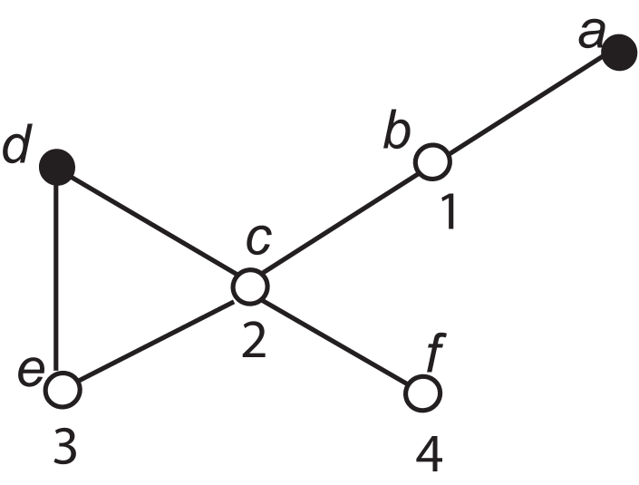
Example 3.26.
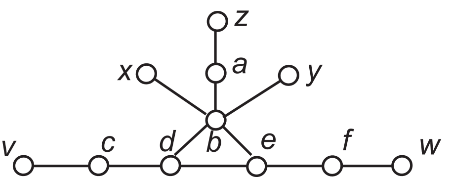
For the graph in Figure 9, . Every minimum zero forcing set must contain one of and one of ; without loss of generality, . If then ; if not then or is in and . Thus is in every efficient zero forcing set.
Proposition 3.27.
Let be a graph and . If and , then .
Proof.
Suppose , and let be an efficient set of forces of . Then performs a force in the efficient set of . Since every force is performed at time 1, . ∎
The converse of Proposition 3.27 is false, as the next example demonstrates.
Example 3.28.
Let be the graph in Figure 10.
It can be verified that . Then and are minimum zero forcing sets and , so . Let be a zero forcing set of not containing vertex . In order to have , some neighbor of must be able to force immediately. Without loss of generality, this neighbor is . Then . The set is a minimum zero forcing set but has propagation time , because no vertex can force immediately. Thus , and observe that .
4 Relationship of propagation time and diameter
In general, the diameter and the propagation time of a graph are not comparable. Let be the dart (shown in Figure 2). Then . On the other hand, .
Although it is not possible to a obtain a direct ordering relationship between diameter and propagation time in an arbitrary graph, diameter serves as an upper bound for propagation time in the family of trees. To demonstrate this, we need some definitions. The walk in is the subgraph with vertex set and edge set (vertices and/or edges may be repeated in these lists but are not repeated in the vertex and edge sets). A trail is a walk with no repeated edges (vertices may be repeated; a path is a trail with no repeated vertices). The length of a trail , denoted by , is the number of edges in . We show in Lemma 4.1 below that for any graph and minimum zero forcing set , there is a trail of length at least . A trail produced by the method in the proof is illustrated in the Example 4.2 below.
Lemma 4.1.
Let be a graph and let be a minimum zero forcing set of . Then there exists a trail such that .
Proof.
Observe that if such that forces at time , then cannot force at time . Thus either was forced at time or some neighbor of was forced at time . So there is a path , where forces at time , or a path , where forces at time and is a neighbor of .
We construct a trail , such that for each time , , there exists an , , such that forces at time . Begin with and work backwards to to construct the trail, using negative numbering. To start, there is some vertex that is forced by a vertex at time ; the trail is now . Assume the trail has been constructed so that for each time , there exists an , such that forces at time . If , then at . Thus either or is a path in , and we can extend our trail to or . It should be obvious that no forcing edge will appear in this walk multiple times (by our construction). If is not a forcing edge, then it can only appear in our walk if forced and forced . Let be the first occurrence of in our walk. If were to occur again, either or would need to be forced at this later time, but this cannot happen because and are both black at this point. ∎
Example 4.2.
Let be the graph in Figure 11. As shown by the numbering in the figure, , but does not contain a path of length 4. The trail produced by the method of proof used in Lemma 4.1 is and has length 6.
Theorem 4.3.
Let be a tree and be a minimum zero forcing set of . Then . Hence, .
Proof.
Choose to be a minimum zero forcing set such that . By Lemma 4.1, there exists a trail in of length at least . Since between any two vertices in a tree there is a unique path, any trail is a path and the diameter of must be the length of the longest path in . Therefore,
The diameter of a graph can get arbitrarily larger than its minimum propagation time. The next example exhibits this result, but first we observe that if is a graph having exactly leaves, then since at most two leaves can be on a maximal forcing chain.
Example 4.4.
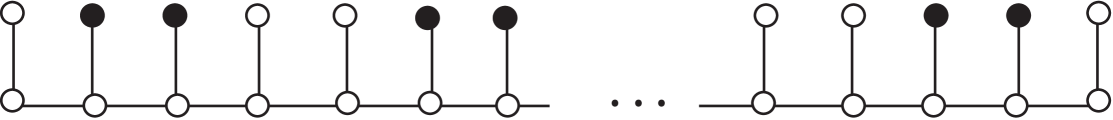
To construct a -comb, we append a leaf to each vertex of a path on vertices, as shown in Figure 12 (our -comb is the special case of a more general type of a comb defined in [8]). Let denote a -comb where . It is clear that . If we number the leaves in path order starting with one, then the set consisting of every leaf whose number is congruent to 2 or 3 (shown in black in the Figure 12) is a zero forcing set, and . Since , is a minimum zero forcing set. Then . Since , , and , . Therefore, . Thus the is arbitrarily larger than .
Acknowledgement The authors thank the referees for many helpful suggestions.
References
- [1] AIM Minimum Rank – Special Graphs Work Group (F. Barioli, W. Barrett, S. Butler, S. M. Cioabă, D. Cvetković, S. M. Fallat, C. Godsil, W. Haemers, L. Hogben, R. Mikkelson, S. Narayan, O. Pryporova, I. Sciriha, W. So, D. Stevanović, H. van der Holst, K. Vander Meulen, A. Wangsness). Zero forcing sets and the minimum rank of graphs. Linear Algebra and its Applications, 428: 1628–1648, 2008.
- [2] F. Barioli, W. Barrett, S. Fallat, H. T. Hall, L. Hogben, B. Shader, P. van den Driessche, H. van der Holst. Zero forcing parameters and minimum rank problems. Linear Algebra and its Applications 433: 401–411, 2010.
- [3] D. Burgarth and V. Giovannetti. Full control by locally induced relaxation. Physical Review Letters PRL 99, 100–501, 2007.
- [4] K. B. Chilakamarri, N. Dean, C. X. Kang, E. Yi. Iteration Index of a Zero Forcing Set in a Graph. Bulletin of the Institute of Combinatorics and its Applications, 64: 57–72, 2012.
- [5] C. J. Edholm, L. Hogben, M. Huynh, J. Lagrange, D. D. Row. Vertex and edge spread of zero forcing number, maximum nullity, and minimum rank of a graph. Linear Algebra and its Applications, in press.
- [6] L. Hogben. Minimum rank problems. Linear Algebra and its Applications, 432: 1961–1974, 2010.
- [7] D. D. Row. A technique for computing the zero forcing number of a graph with a cut-vertex. Linear Algebra and its Applications, in press.
- [8] S. Severini. Nondiscriminatory propagation on trees. Journal of Physics A, 41: 482002 (Fast Track Communication), 2008.