Properties of two level systems in current-carrying superconductors

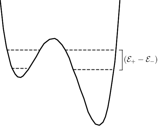
The concept of two-level systems (TLS) was introduced to explain the unusual thermal and transport properties of insulating and metallic glasses [1, 2] (see Refs. [3, 4, 5, 6, 7, 8] for a review of the subject). While the microscopic nature of TLS is still not fully understood, the standard phenomenological model assumes the ability for an atom, or several atoms, to tunnel quantum mechanically at low temperatures between two quasi-stable atomic configurations, as illustrated in Fig. 1.

The dynamics of TLS may be described by a $2\times 2$ matrix Hamiltonian of the form

$\displaystyle\hat{H}_{0}=\begin{pmatrix}\epsilon&t\\ t^{*}&-\epsilon\\ \end{pmatrix}.$

(1)

Here $2\epsilon$ is the energy difference between the two quasi-stable configurations and $t$ is the tunneling amplitude between them. Diagonalization of this Hamiltonian yields the eigenvalues of the system

$$\mathcal{E}_{\pm}=\pm\sqrt{\epsilon^{2}+|t|^{2}}.$$

(2)

External perturbations modify the parameters of the Hamiltonian. Usually, it is assumed that the modulation of the inter-well splitting $\epsilon$ is much bigger than the modulation of $t$ (see for example Ref [7]). Thus, the coupling of TLS to external low frequency perturbations is described by the time-dependence of the inter-well energy splitting $\epsilon(t)=\epsilon_{0}+\delta\epsilon(t)$. For example, in the presence of an external electric field ${\bf E}(t)$ we have a “dipole” contribution to the energy splitting,

$\displaystyle\delta\epsilon_{d}(t)=$

$\displaystyle\,-{\bf E}(t)\cdot{\bf d},$

(3)

where $2{\bf d}$ is the dipole moment difference between the two metastable states of the TLS whose magnitude and direction are random. The coupling of this form changes both the eigenvalues $\mathcal{E}_{\pm}$ and the eigenfunctions, and therefore adequately describes both resonant and relaxation absorption mechanisms of the electric field by the TLS.

The TLS has also been suggested as a source of the ubiquitous $1/\mathrm{f}$ noise in conductors (see for example [9, 10, 11, 12]). Since the two states of the TLS have different electron scattering cross-sections, transitions between them change the local conductivity. If the distribution function of TLS relaxation times is broad, the $1/\mathrm{f}$ noise of current fluctuations through a voltage-biased sample can be attributed to fluctuations in sample conductance induced by the TLS transitions. This picture has been confirmed by measuring “noise of the noise” in metals [13].

At low temperatures $T$, the quantum interference of electron waves in metals results in large sensitivity of electron transport to the motion of individual scatterers [14, 15]. At relatively weak magnetic fields, the electron system crosses over from the “orthogonal” to the “unitary” ensemble and, as a result, the amplitude of the $1/\mathrm{f}$ noise is suppressed by a factor two  [15, 16]. Conversely, due to the interaction of TLS with the Friedel oscillations of the electron density, the properties of TLS in metals at low temperatures are strongly affected by the quantum interference of the electron wave functions, resulting in a strong dependence of the TLS activation energy on the magnetic field [17]. This phenomenon was revealed by measurements of the magnetic field dependence of the plateaus in the telegraph signal associated with transitions between the two states of a single fluctuator [18, 19]. Thus, the strong interaction of TLS with the local density of electrons in disordered conductors has been verified experimentally.

In disordered $s$-wave superconductors, the TLS become the most abundant low-energy excitations at low temperatures and thus play important role in the dissipation and decoherence of superconducting systems. Since the typical size of TLS is believed to be smaller than the superconducting coherence length $\xi$, their atomic structure and strength of coupling to the electron density should be similar to that in normal metals.

In this article, we consider the effect of superconducting pairing on the coupling of TLS to the external ac electric field ${\bf E}(t)=\mathrm{Re}\large({\bf E}_{\omega}e^{-i\omega t}\large)$. We show that in the presence of a dc supercurrent and at sufficiently small frequencies, the effective interaction between the TLS and the electromagnetic field is parametrically enhanced. The physical origin of this effect lies in the large sensitivity of the random Friedel oscillations of the electron density $n({\bf r},{\bf p}_{s})$ in disordered superconductors to the changes of the superfluid momentum

$${\bf p}_{s}(t)=\frac{\hbar}{2}\bm{\nabla}\chi-\frac{e}{c}{\bf A}(t).$$

(4)

Here $\chi({\bf r},t)$ is the phase of the superconductiviting order parameter, and ${\bf A}(t)$ is the vector potential. The inter-well energy splitting $\epsilon(t)$ of the TLS is affected by the interaction of the atoms forming TLS with the electron density. Therefore it acquires a ${\bf p}_{s}$-dependent correction $\delta\epsilon_{s}$. Since atomic TLS do not break time reversal invariance, their energy must be an even function of ${\bf p}_{s}$. Therefore, at small supercurrent densities this correction can be written in the form

$\displaystyle\delta\epsilon_{s}(t)=$

$\displaystyle\,\alpha_{s}\,p_{s}^{2}(t),\quad\alpha_{s}\equiv\left.\frac{d\epsilon(p_{s}^{2})}{d\left(p_{s}^{2}\right)}\right|_{p_{s}^{2}=0}.$

(5)

In the presence of an ac electric field the superfluid momentum becomes time-dependent,

$$\dot{{\bf p}}_{s}(t)=e{\bf E}(t).$$

(6)

This causes time-dependence of the TLS Hamiltonian in Eq. (1). Equation (5) shows that a linear coupling of the external electric field to TLS mediated by superconductive pairing is possible only in the presence of a dc superfluid momentum $\bar{\bf p}_{s}$. In this case, the time-dependent superfluid momentum can be written as ${\bf p}_{s}(t)=\bar{{\bf p}}_{s}+\delta{\bf p}_{s}(t)$, where, according to Eq. (6), $\delta{\bf p}_{s}(t)=\mathrm{Re}\large(ie{\bf E}_{\omega}e^{-i\omega t}/\omega\large)$.

The instantaneous relation between the time-dependent superfluid momentum ${\bf p}_{s}(t)$ and the energy splitting described by Eq. (5) remains valid as long as $\omega\ll\Delta$. Combining Eq. (3) with Eq. (5), linearized with repect to $\delta{\bf p}_{s}$, we find that in this frequency interval, the interaction of TLS with an ac electric field in current-carrying superconductors has the form $\delta\epsilon(t)=\Re\left(\delta\epsilon_{\omega}e^{-i\omega t}\right)$ where

$\displaystyle\delta\epsilon_{\omega}=$

$\displaystyle\,-\left(\bm{d}-i\frac{e}{\omega}\alpha_{s}\bar{\bf p}_{s}\right)\cdot{\bf E}_{\omega}.$

(7)

Although Eqs. (5) and (7) can be introduced phenomenologically, evaluation of the parameter $\alpha_{s}$, which characterizes the sensitivity of TLS level splitting to the superfluid momentum, requires a microscopic consideration.

Below, we develop a microscopic theory of this effect for s-wave superconductors in the diffusive regime, where the coherence length $\xi$ is larger than the electron mean free path $\ell$ in the normal state, $\xi=\sqrt{D/\Delta}>\ell>\lambda_{F}$. Here $\Delta$ is the superconducting gap, $D=v_{F}\ell/3$ is the diffusion coefficient, $v_{F}$ is the Fermi velocity, and $\lambda_{F}$ is the Fermi wavelength. In this case, the magnitude of the parameter $\alpha_{s}$ is large because of the high sensitivity of the Friedel oscillations of the electron density to the changes in $p_{s}$. We assume that the typical kinetic and potential energy of electrons in the system are of the same order, $r_{s}=e^{2}/\hbar v_{F}\sim 1$, and that the characteristic size of TLS is of the order of the interatomic spacing, which in metals is of the order of $\lambda_{F}$. In this case, the $p_{s}$-dependent correction to inter-well energy splitting $\delta\epsilon_{s}$ in Eq. (5) may be estimated as

$$\delta\epsilon_{s}(t)\sim e\lambda_{F}\delta n({\bf r},{\bf p}_{s}(t)),$$

(8)

where $\delta n({\bf r},{\bf p}_{s}(t))$ is the $p_{s}$-dependent correction to the electron density. Thus, the parameter $\alpha_{s}$ in Eqs. (5) and (7) can be expressed in terms of the sensitivity of the variations of the electron density $\delta n({\bf r},{\bf p}_{s}(t))$ to the superfluid momentum. This enables us to evaluate the coupling of TLS to ac electric fields and all subsequent quantities within a factor of order unity.

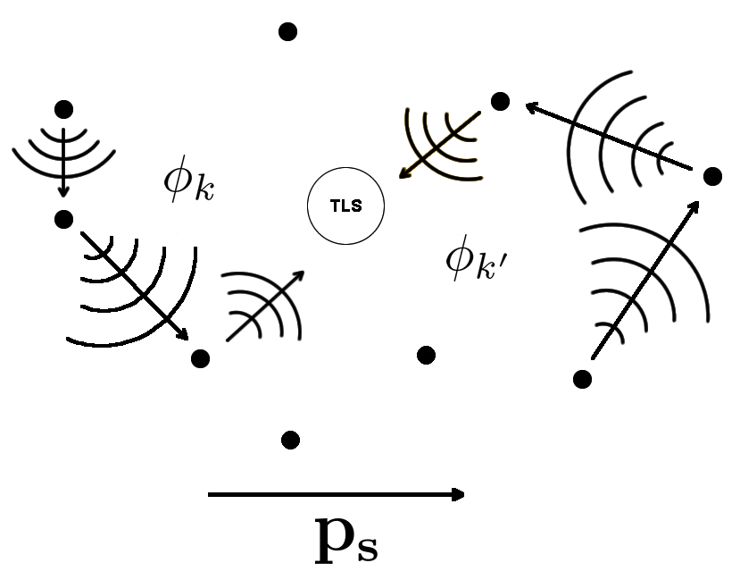
For simplicity, we consider the situation where a superconducting film with a thickness $L_{z}$ smaller than the skin length is exposed to a monochromatic ac electric field of frequency $\omega$. The spatial modulations of the electron density $n({\bf r})$, which contribute to the TLS level splitting are caused by the interference of the electronic waves scattered by different impurities. Due to the rapid decay of the Friedel oscillation amplitude with the distance from the impurity, the value of $n({\bf r})$ is determined primarily by impurities closest to the TLS. However, the sensitivity of the electron density to the changes in ${\bf p}_{s}$ is determined by the interference of quantum amplitudes for the electron propagation from the impurities separated from the observation point by distances of order $\xi$. This can be understood as follows: At ${\bf p}_{s}\neq 0$, the electron amplitudes corresponding to different diffusion paths acquire random phases $\delta\phi_{k}\sim\int{\bf p}_{s}\cdot d{\bf l}_{k}$, where the index $k$ labels different diffusion paths. This changes the interference of contributions of different paths to the electron density. Since $\delta\phi_{k}$ increases with the length of the path, the sensitivity of the electron density $\delta n({\bf r},{\bf p}_{s})=n({\bf r},0)-n({\bf r},{\bf p}_{s})$ is controlled by contributions from electron waves traveling from impurities situated at distances of the order of the superconducting correlation length $\xi$ from point ${\bf r}$. This is shown qualitatively in Fig. 2. Therefore, the variance of $\delta n({\bf r},{\bf p}_{s})$ in the diffusive regime can be obtained using the standard diagram technique of averaging over random impurity potential [20], valid at $\lambda_{F}\ll\ell$. To be concrete, we consider thin films of thickness smaller than the coherence length, $\lambda_{F}<L_{z}<\xi$. Evaluating the Feynman diagrams shown in Fig. 3, we get

$\displaystyle\sqrt{\langle(\delta n)^{2}({\bf r},{\bf p}_{s})\rangle}=\frac{C}{\lambda_{F}^{3}\sqrt{G}}\frac{\Delta}{\epsilon_{F}}\left(\frac{p_{s}}{p_{d}}\right)^{2},\quad p_{s}\ll p_{d}.$

(9)

Here $\langle\ldots\rangle$ denotes averaging over disorder, $\epsilon_{F}$ is the Fermi energy, $p_{d}=\sqrt{\Delta/D}$ is the depairing superfluid momentum, $C$ is a numerical factor of order unity, and

$$G=\frac{8\pi}{3}\frac{\ell L_{z}}{\lambda_{F}^{2}}$$

(10)

is the conductance of the film in units of $e^{2}/2\pi\hbar$.

Using Eq. (9) we obtain the following estimates for the variances of $\delta\epsilon_{s}(t)$ in Eq. (8), and the parameter $\alpha_{s}$ in Eqs. (5) and (7),

	$\displaystyle\sqrt{\langle(\delta\epsilon_{s})^{2}\rangle}\sim$	$\displaystyle\,|\Delta|\frac{1}{\sqrt{G}}\left(\frac{p_{s}}{p_{d}}\right)^{2}=\frac{1}{\sqrt{G}}Dp_{s}^{2},$		(11a)
	$\displaystyle\sqrt{\langle\alpha_{s}^{2}\rangle}\sim$	$\displaystyle\,\frac{D}{\sqrt{G}},\quad\langle\alpha_{s}\rangle=0.$		(11b)

These results show that in situations where the electric field is not orthogonal to $\bar{{\bf p}}_{s}$, the ratio of the second and the first terms in the brackets in Eq. (7) is of order

$$\frac{e\alpha_{s}\bar{p}_{s}}{\omega d}\sim\frac{\omega{*}}{\omega}.$$

(12)

Here we introduced the characteristic frequency scale defined by the dc superfluid momentum

$$\omega^{*}=\Delta\frac{\bar{p}_{s}}{p_{d}}\sqrt{\frac{\xi_{0}}{L_{z}}},$$

(13)

with $\xi_{0}=v_{F}/\Delta$ being the coherence length of pure superconductor. It follows from Eqs. (7), and (12) that for

$$\omega<\omega^{*}.$$

(14)

The interaction between the TLS and the external electric field is dominated by the temporal oscillations of the electron density, rather than by the direct interaction of the external electric field with the dipolar moment of the TLS.

The aforementioned $\bar{{\bf p}}_{s}$-dependent enhancement of the coupling of TLS to electric fields manifests itself in all ac phenomena. This includes resonant absorption, absorption related to the relaxation mechanism, and all nonlinear effects. The frequency dependences of these effects will be very different from the conventional ones.

Equations (5), (7) and (11) show that in the presence of supercurrent, the dissipative part of the conductivity tensor becomes anisotropic. The enhancement of TLS coupling to ac electric fields occurs only for the longitudinal geometry, where the ac electric field is parallel to $\bar{\bf p}_{s}$. At small $\omega$, the corresponding longitudinal component of the dissipative conductivity, $\sigma_{\|}$, is significantly enhanced as compared to the $\bar{\bf p}_{s}=0$ case. In contrast, the transverse component $\sigma_{\perp}$ remains roughly the same as that at $\bar{\bf p}_{s}=0$.

As an example, we evaluate the TLS contribution to the dissipative part of the longitudinal microwave conductivity at sufficiently small frequencies, where it is controlled by the Debye relaxation mechanism (see, for example, [21, 7, 22, 23]). Energy dissipation in the relaxation mechanism is caused by the time-dependence of the TLS energy levels, which creates a non-equilibrium level population, whose relaxation leads to entropy production. In this case the main contribution to the absorption power $P=\sigma_{\|}E^{2}_{\omega}/2$ comes from the TLS with $|\mathcal{E}_{+}-\mathcal{E}_{-}|\lesssim T$, and long relaxation times, $\tau\sim 1/\omega$. The latter condition corresponds to $|t|\ll|\epsilon|$ in Eqs. (1), and (2), which implies $|\mathcal{E}_{+}-\mathcal{E}_{-}|\approx 2|\epsilon|$. Using standard arguments (see for example [22]), we get the following estimate for the dissipative part of the longitudinal conductivity

$$\sigma_{\|}(\omega)\sim e^{2}\nu(T)\int d\tau f(\tau)\frac{\lambda_{F}^{2}\tau\left[\omega^{2}+\eta\cdot(\omega^{*})^{2}\right]}{1+(\omega\tau)^{2}}.$$

(15)

Here $\nu(T)$ is the density of states of TLS with $\epsilon\sim T$ per unit area, $f(\tau)$ is the distribution function of relaxation times normalized to unity, and $\eta\sim 1$ is a factor of order one. In general, $\nu(T)$ is temperature-dependent. However, we note that in glasses this quantity does not depend on $T$.

At $T\ll\Delta$ the concentration of quasiparticles in s-wave superconductors is exponentially small, and the TLS relaxation times are controlled by their interactions with phonons, similar to the case of dielectrics. The frequency dependence of the conductivity depends on how quickly $f(\tau)$ decays at large values of $\tau$. If $f(\tau\rightarrow\infty)$ decays quicker than $1/\tau^{2}$ then one can introduce a characteristic relaxation time $\tilde{\tau}$. In this case at $p_{s}=0$ the conductivity, $\sigma(\omega)\sim e^{2}\nu\lambda_{F}^{2}\omega^{2}\tilde{\tau}$, is isotropic and quadratic in frequency. However, at $\bar{{\bf p}}_{s}\neq 0$ and $\omega\ll\omega^{*}$, the longitudinal component of the conductivity tensor, $\sigma_{\|}(\omega)$, exhibits a giant enhancement, proportional to the parameter $(\omega^{*}/\omega)^{2}$. In this case

$$\sigma_{\|}(\omega\rightarrow 0){\color[rgb]{0,0,1}{\sim}}e^{2}\nu(\lambda_{F}\omega^{*})^{2}\tilde{\tau}$$

(16)

becomes frequency-independent.

In many disordered systems, especially in glasses, the relaxation time of TLS has an exponential dependence, $\tau\sim\exp(\zeta)$, on some parameter $\zeta$, which is uniformly distributed. In such cases the distribution function $f(\tau)$ is broad, and has the form (see for example [10, 11]),

$$f(\tau)\sim 1/\tau.$$

(17)

Then, according to Eq. (15) at $\bar{\bf p}_{s}=0$ has a linear dependence on the frequency,

$$\sigma(\omega)\sim e^{2}\nu\lambda_{F}^{2}\omega.$$

(18)

In contrast, at $\bar{p}_{s}\neq 0$ , and $\omega\ll\omega^{*}$ the longitudinal conductivity is inversely proportional to $\omega$,

$$\sigma_{\|}(\omega)\sim e^{2}\nu\frac{(\lambda_{F}\omega^{*})^{2}}{\omega}.$$

(19)

It may seem counter-intuitive that according to Eq. (15), at $\bar{p}_{s}\neq 0$ the conductivity associated with localized TLS does not vanish as $\omega\rightarrow 0$. The reason for this is as follows. Inelastic processes induce transitions between the two states of TLS and modulate the supercurrent by changing the superfluid density. At low frequencies, this modulation turns out to be in phase with the oscillations of the external electric field, leading to dissipation.

Since a superconductor carrying a dc supercurrent is in an equilibrium state, one can use the fluctuation-dissipation theorem (FDT) [24] to relate the spectral density of fluctuations of the total current through the system to the dissipative conductivity $\sigma_{\parallel}(\omega)$,

$$S_{s}(\omega)=\int dt\overline{\delta I_{s}(t)\delta I_{s}(0)}e^{i\omega t}=T\sigma_{\|}(\omega),\,\,\,\,\,\,\ \omega<T.$$

(20)

Here the subscript $s$ indicates that the system is in the superconducting state and $\delta I_{s}(t)$ describes fluctuations component of the total current in the direction of $\bar{{\bf p}}_{s}$.

It follows from Eqs. (15), and (20) that in the presence of super-current, and at $\omega<\omega^{*}$ the amplitude of the current fluctuations exhibits giant enhancement. In particular, according to Eqs. (19), (20), in systems where $f(\tau)\sim 1/\tau$ the current correlation function has 1/f form

$$S_{s}(\omega)\sim\Gamma\frac{I_{s}^{2}}{V\omega},\,\,\,\,\,\,\,\,\ \Gamma=\frac{\nu T\ell}{\langle N_{s}\rangle^{2}}.$$

(21)

Here $I_{s}$ is the total bias supercurrent passing through the system, and we used the relation between the average supercurrent density and superfluid density per unit area $\langle{\bf j}_{s}\rangle=e\langle N_{s}\rangle{\bf p}_{s}/m$, which is valid at $p_{s}\ll p_{d}$.

The expression for the spectral density of current fluctuations in Eq. (21) describing $1/\mathrm{f}$ noise in superconductors is similar to the corresponding expression for the $1/\mathrm{f}$ noise of normal current in metals (see for example [10, 11]). In both cases the spectral functions are quadratic in the dc current and inversely proportional to the volume of the sample. However, there are significant differences between these two situations.

In normal metals, the $1/\mathrm{f}$ noise of the total current is related to the conductance fluctuations and exists only in the presence of a bias current. These current fluctuations are non-equilibrium and therefore do not obey the fluctuation-dissipation theorem. In particular, at $\omega\to 0$ the conductivity of metals becomes frequency-independent. In contrast, Eq. (21) describes equilibrium current fluctuations, and the divergence of $S_{s}(\omega)$ at $\omega\rightarrow 0$ is accompanied by the corresponding divergence of the conductivity in Eq. (19).

According to Eqs. (18) and (19), the spectrum of the current fluctuations in superconductors is dominated by the $1/\mathrm{f}$ noise for $\omega<\omega^{*}$. This frequency interval can be significantly larger than the interval in which the $1/\mathrm{f}$ noise exceeds the equilibrium Johnson-Nyquist noise in the normal metals.

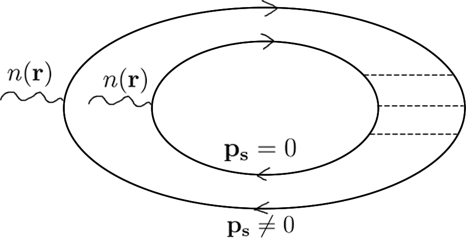
Equations (5), (7) and (11) can be obtained from an alternative consideration by evaluating the sensitivity of the superfluid density per unit area, $N_{s}$, to a change of state of the TLS. It was shown in Refs. [25, 26, 27] that the r.m.s. the amplitude of its mesoscopic fluctuations, of the superfluid density $\delta N_{s}=N_{s}-\langle N_{s}\rangle$, averaged over a region of size $\xi$, scales with the amplitude of universal conductance fluctuations [14, 28] of the sample,

$\displaystyle\sqrt{\langle(\delta N_{s})^{2}\rangle}\sim$

$\displaystyle\,\langle N_{s}\rangle/G\sim N\lambda_{F}(\Delta/\epsilon_{F}).$

(22)

Here $N$ is the electron density, and we used the expression for average superfluid density per unit area $\langle N_{s}\rangle\sim NL_{z}\ell/\xi_{0}$.

By changing the electron interference pattern, transitions of an individual TLS located at $\bm{r}_{i}$ induce time-dependence of the superfluid density in the spacial region of the order of the coherence length $\xi$ near $\bm{r}_{i}$. We denote the time-dependent part of the superfluid density averaged over this region by $\delta N_{s}({\bf r}_{i},t)\equiv\tilde{N}_{s,i}(t)$. At $r_{s}\sim 1$ the difference in the electron scattering amplitudes in the two different states of a TLS is of the order of $\lambda_{F}^{2}$. Therefore, using Eq. (22) the r.m.s. value of a random change of the superfluid density caused by a change of state of an individual TLS may be estimated as ¹¹1The estimate (23) can be obtained as follows. It was shown in Refs. [14, 15] (see also Ref. [27] for a review) that the number of impurities $n_{0}$ whose scattering amplitude needs to be changed by $\delta f\sim\lambda_{F}$ in order to change the conductance by $\delta G\sim e^{2}/\hbar$, (and consequently the superfluid density by $\delta N_{s}$) is of order $n_{0}\sim G$. The qualitative explanation of this fact is as follows. The mesoscopic fluctuations of $\delta N_{s}$ originate from the interference of diffusion paths traveling across a region of size $\xi$. Each diffusive path can be viewed as a tube with a cross-section area $\sim\lambda_{F}^{2}$ surrounding a classical diffusive trajectory with a typical length $\xi^{2}/\ell$. Thus, its volume is of the order of $v=\xi^{2}\lambda_{F}^{2}/\ell$. The interference pattern changes completely if each diffusion path contains at least one impurity which changes its scattering amplitude. Thus $n_{0}\sim\frac{V}{v}=G$ , where $V=\xi^{2}L_{z}$ is the volume of a sample of a lateral size $\xi$. Since the changes of the superfluid density associated with motions of individual scatterers have random signs, the estimate for the r.m.s. value of $\delta\tilde{N}_{s}$, Eq. (23) is obtained by dividing $\delta N_{s}$ in Eq. (22) by $\sqrt{n_{0}}$.

$$\sqrt{(\delta\tilde{N}_{s,i})^{2}}\sim\frac{\sqrt{(\delta N_{s})^{2}}}{\sqrt{G}}.$$

(23)

Finally, associating the change of the energy of the TLS with the change of the superfluid energy of a block of size $\xi$, $\delta\epsilon({\bf p}_{s})=\xi^{2}\delta\tilde{N}_{s}{\bf p}_{s}^{2}/m$, we reproduce Eq. (11a).

Using Eqs. (22), (23) we can also obtain the spectrum of the $1/\mathrm{f}$ current noise in Eqs. (19), (20), (21) without appealing to FDT. This consideration elucidates the microscopic origin of the current noise in current-carrying superconductors, by tracing them to the temporal fluctuations of the superfluid density, $\delta\tilde{N}_{s}({\bf r},t)$, which are induced by the TLS transitions.

On the spacial scales larger than $\xi$, the superfluid density can be written as

$$N_{s}({\bf r},t)-\langle N_{s}\rangle=\sum_{i}\delta\tilde{N}_{s,i}(t)\xi^{2}\delta({\bf r}-{\bf r}_{i}).$$

(24)

Here the index $i$ labels individual TLS. Assuming that transitions of different TLS are uncorrelated, we get the spectrum of fluctuations of $\delta\tilde{N}_{s,i}(t)$ in the form

$$\int dt\overline{\delta\tilde{N}_{s,i}(t)\tilde{N}_{s,j}(0)}e^{i\omega t}=\delta_{ij}\frac{\tau_{i}\,\langle(\delta\tilde{N}_{s})^{2}\rangle}{\pi\left[1+(\omega\tau_{i})^{2}\right]}.$$

(25)

The local current density ${\bf J}_{s}({\bf r},t)=\langle{\bf J}_{s}\rangle+\delta{\bf J}_{s}({\bf r},t)$ and superfluid momentum ${\bf p}_{s}({\bf r},t)={\bf\bar{p}}_{s}+\delta{\bf p}_{s}({\bf r},t)$ can be determined from the continuity equation $\bm{\nabla}\cdot{\bf J}_{s}=0$, which after directing the average superfluid momentum in $x$-direction, and linearization with respect to small fluctuations, can be written as

$$\langle N_{s}\rangle\,\bm{\nabla}\cdot\delta{\bf p}_{s}({\bf r},t)+\bar{\bf p}_{s}\cdot\bm{\nabla}N_{s}({\bf r},t)=0.$$

(26)

In this form the problem represented by Eqs. (25), (26) becomes equivalent to the problem of current fluctuations in a current bias normal conductor in which the local conductivity fluctuates in space and time [29]. Solving these equations and averaging the result over the distribution of relaxation time with the distribution function $f(\tau_{i})\sim 1/\tau_{i}$ and over the position of $i$-th TLS, ${\bf r}_{i}$, we reproduce Eq. (21).

The central assumption we made in the article is that the TLS are situated inside superconductors with $r_{s}\sim 1$ and that their size is of order interatomic spacing. Therefore the characteristic dipolar moment of the TLS is of order $e\lambda_{F}$, while the electron scattering cross-section difference between two the states of TLS is of order $\lambda_{F}^{2}$. Recently, other pictures of TLS have been proposed, including electronic traps [30, 31], and localized states associated with spacial fluctuations of superconductor order parameter in strongly disordered superconductors [32, 33, 34, 35]. In these cases, either the characteristic size of the TLS is significantly larger than $\lambda_{F}$, or the TLS are situated in an insulator close to the superconductor. Enhancements of the microwave absorption rate and the spectrum of equilibrium fluctuations, which are proportional to $\bar{p}_{s}^{2}/\omega^{2}$, exist in these cases as well. However, in these situations, Eq. (15) will acquire additional small pre-exponential factors.

The enhancement of the linear longitudinal conductivity proportional to $(\omega^{*}/\omega)^{2}$ can be several orders of magnitude larger than unity. Because of this, in a wide interval of frequencies, the dissipative properties of current-carrying superconductors are dominated by the coupling of TLS to the superfluid current. In this frequency interval, the results presented above enable us to evaluate the ac conductivity and the power of $1/\mathrm{f}$ current noise up to a factor of order unity. The linear approximation in the external electric field is valid as long as $eE_{\omega}/\omega\ll\bar{p}_{s}$. In the nonlinear regime, $p_{d}>eE_{\omega}/\omega>\bar{p}_{s}$, Eq. (5) is still valid, and the enhancement of the nonlinear absorption coefficient is independent of $\bar{p}_{s}$.

Finally, we would like to mention that the results presented above may be relevant to the physics of superconductor-insulator-superconductor junctions. In the presence of voltage on the junction the current exhibits oscillations in time which are accompanied by oscillations of superfluid velocity in superconducting leads supplying the current to the junction. Therefore there is a contribution to the total dissipation rate of the system associated with TLS in the bulk of the leads. Acknowledgements: Authors are grateful for helpful conversations with C. Boettcher, A. Burin, M. Feigelman, L. Faoro, L. Ioffe, S. Kubatkin, C. Marcus, J. Pekola, and B. Shklovskii. The work of B.S. is supported by the DARPA grant GR049687, A.A. was supported by the NSF grant DMR-2424364, and the work of T. Liu was supported by NSF Grant No. DMR-2203411.

References

- Anderson et al. [1972] P. w. Anderson, B. I. Halperin, and c. M. Varma, Anomalous low-temperature thermal properties of glasses and spin glasses, The Philosophical Magazine: A Journal of Theoretical Experimental and Applied Physics 25, 1 (1972).
- Phillips [1972] W. A. Phillips, Tunneling states in amorphous solids, Journal of Low Temperature Physics 7, 351 (1972), https://doi.org/10.1080/14786437208229210 .
- Phillips [1987] W. A. Phillips, Two-level states in glasses, Reports on Progress in Physics 50, 1657 (1987).
- Black [1981] J. L. Black, Low-energy excitations in metallic glasses, in Glassy Metals I: Ionic Structure, Electronic Transport, and Crystallization, edited by H.-J. Güntherodt and H. Beck (Springer Berlin Heidelberg, Berlin, Heidelberg, 1981) pp. 167–190.
- Galperin et al. [1989] Y. M. Galperin, V. G. Karpov, and V. I. Kozub, Localized states in glasses, Advances in Physics 38, 669 (1989), https://doi.org/10.1080/00018738900101162 .
- Müller et al. [2019] C. Müller, J. H. Cole, and J. Lisenfeld, Towards understanding two-level-systems in amorphous solids: insights from quantum circuits, Reports on Progress in Physics 82, 124501 (2019).
- Enss and Hunklinger [2005] C. Enss and S. Hunklinger, Low-Temperature Physics, SpringerLink: Springer e-Books (Springer Berlin Heidelberg, 2005).
- Burin et al. [1998] A. L. Burin, D. Natelson, D. D. Osheroff, and Y. Kagan, Interactions between tunneling defects in amorphous solids, in Tunneling Systems in Amorphous and Crystalline Solids, edited by P. Esquinazi (Springer Berlin Heidelberg, Berlin, Heidelberg, 1998) pp. 223–315.
- Dutta and Horn [1981] P. Dutta and P. M. Horn, Low-frequency fluctuations in solids: noise, Rev. Mod. Phys. 53, 497 (1981).
- Kogan [1996] S. Kogan, Electronic Noise and Fluctuations in Solids (Cambridge University Press, 1996).
- Weissman [1988] M. B. Weissman, noise and other slow, nonexponential kinetics in condensed matter, Rev. Mod. Phys. 60, 537 (1988).
- Paladino et al. [2014] E. Paladino, Y. M. Galperin, G. Falci, and B. L. Altshuler, 1/f noise: Implications for solid-state quantum information, Rev. Mod. Phys. 86, 361 (2014).
- Voss and Clarke [1976] R. F. Voss and J. Clarke, Flicker () noise: Equilibrium temperature and resistance fluctuations, Phys. Rev. B 13, 556 (1976).
- Altshuler and Spivak [1985] B. L. Altshuler and B. Z. Spivak, Variation of the random potential and the conductivity of samples of small dimensions, JETP Lett. 42 (1985).
- Feng et al. [1986] S. Feng, P. A. Lee, and A. D. Stone, Sensitivity of the conductance of a disordered metal to the motion of a single atom: Implications for noise, Phys. Rev. Lett. 56, 1960 (1986).
- Birge et al. [1989] N. O. Birge, B. Golding, and W. H. Haemmerle, Electron quantum interference and noise in bismuth, Phys. Rev. Lett. 62, 195 (1989).
- Al’Tshuler and Spivak [1989] B. Al’Tshuler and B. Spivak, Effect of magnetic field on the dynamics of impurities in metallic systems, Jetp Letters - JETP LETT-ENGL TR 49 (1989).
- Chun and Birge [1993] K. Chun and N. O. Birge, Dissipative quantum tunneling of a single defect in bi, Phys. Rev. B 48, 11500 (1993).
- Chun and Birge [1996] K. Chun and N. O. Birge, Dissipative quantum tunneling of a single defect in a disordered metal, Phys. Rev. B 54, 4629 (1996).
- Abrikosov et al. [1975] A. A. Abrikosov, I. Dzyaloshinskii, L. P. Gorkov, and R. A. Silverman, Methods of quantum field theory in statistical physics (Dover, New York, NY, 1975).
- Debye [1970] P. Debye, Polar molecules, Dover books on chemistry and physical chemistry (Dover Publ., 1970).
- Shklovskii and Efros [1981] B. I. Shklovskii and A. L. Efros, Zero-phonon ac hopping conductivity of disordered systems, Sov. Phys. JETP 54, 218 (1981).
- Efros [1981] A. L. Efros, On the theory of a.c. conduction in amorphous semiconductors and chalcogenide glasses, Philosophical Magazine B 43, 829 (1981), https://doi.org/10.1080/01418638108222349 .
- Lifshitz and Pitaevskii [2013] E. Lifshitz and L. Pitaevskii, Statistical Physics: Theory of the Condensed State, Course of Theoretical Physics No. v. 9 (Butterworth-Heinemann, 2013).
- Al’tshuler and Spivak [1987] B. L. Al’tshuler and B. Z. Spivak, Mesoscopic fluctuations in a superconductor-normal metal-superconductor junction, Soviet Journal of Experimental and Theoretical Physics 65, 343 (1987).
- Spivak and Zyuzin [1988] B. Z. Spivak and A. Y. Zyuzin, Mesoscopic fluctuations of the superfluidcurrent density in disordered superconductors, JETP Lett 47, 270 (1988).
- Spivak and Zyuzin [1991] B. Spivak and A. Zyuzin, Chapter 2 - mesoscopic fluctuations of current density in disordered conductors, in Mesoscopic Phenomena in Solids, Modern Problems in Condensed Matter Sciences, Vol. 30, edited by B. ALTSHULER, P. LEE, and R. WEBB (Elsevier, 1991) pp. 37–80.
- Lee and Stone [1985] P. A. Lee and A. D. Stone, Universal conductance fluctuations in metals, Phys. Rev. Lett. 55, 1622 (1985).
- Altshuler and Spivak [1989] B. L. Altshuler and B. Z. Spivak, Fluctuations in the intensity of 1/f noise in disordered metals, JETP Lett. 49, 527 (1989).
- Koch et al. [2007] R. H. Koch, D. P. DiVincenzo, and J. Clarke, Model for flux noise in squids and qubits, Phys. Rev. Lett. 98, 267003 (2007).
- Lupaşcu et al. [2009] A. Lupaşcu, P. Bertet, E. F. C. Driessen, C. J. P. M. Harmans, and J. E. Mooij, One- and two-photon spectroscopy of a flux qubit coupled to a microscopic defect, Phys. Rev. B 80, 172506 (2009).
- Faoro and Ioffe [2008] L. Faoro and L. B. Ioffe, Microscopic origin of low-frequency flux noise in josephson circuits, Phys. Rev. Lett. 100, 227005 (2008).
- de Graaf et al. [2020] S. E. de Graaf, L. Faoro, L. B. Ioffe, S. Mahashabde, J. J. Burnett, T. Lindström, S. E. Kubatkin, A. V. Danilov, and A. Y. Tzalenchuk, Two-level systems in superconducting quantum devices due to trapped quasiparticles, Science Advances 6, eabc5055 (2020), https://www.science.org/doi/pdf/10.1126/sciadv.abc5055 .
- Khvalyuk et al. [2024] A. V. Khvalyuk, T. Charpentier, N. Roch, B. Sacépé, and M. V. Feigel’man, Near power-law temperature dependence of the superfluid stiffness in strongly disordered superconductors, Phys. Rev. B 109, 144501 (2024).
- Kristen et al. [2024] M. Kristen, J. N. Voss, M. Wildermuth, A. Bilmes, J. Lisenfeld, H. Rotzinger, and A. V. Ustinov, Giant two-level systems in a granular superconductor, Phys. Rev. Lett. 132, 217002 (2024).