Prospects for measuring the Hubble constant and dark energy using gravitational-wave dark sirens with neutron star tidal deformation
Abstract
Using the measurements of tidal deformation in the binary neutron star (BNS) coalescences can obtain the information of redshifts of gravitational wave (GW) sources, and thus actually the cosmic expansion history can be investigated using solely such GW dark sirens. To do this, the key is to get a large number of accurate GW data, which can be achieved with the third-generation (3G) GW detectors. Here we wish to offer an answer to the question of whether the Hubble constant and the equation of state (EoS) of dark energy can be precisely measured using solely GW dark sirens. We find that in the era of 3G GW detectors dark siren data (with the NS tidal measurements) could be obtained in three-year observation if the EoS of NS is perfectly known, and thus using only dark sirens can actually achieve the precision cosmology. Based on a network of 3G detectors, we obtain the constraint precisions of and for the Hubble constant and the constant EoS of dark energy , respectively; for a two-parameter EoS parametrization of dark energy, the precision of is and the error of is 0.13. We conclude that 3G GW detectors would lead to breakthroughs in solving the Hubble tension and revealing the nature of dark energy provided that the EoS of NS is perfectly known.
1 Introduction
Allan Sandage pointed out in as early as 1970 that the two key numbers that should be precisely measured in cosmology are the Hubble constant () and the deceleration parameter () [1]. This is undoubtedly a deep insight. The measurement of using type Ia supernovae has led to the discovery of the accelerating expansion of the universe [2, 3], which is usually explained through assuming an exotic component with a negative pressure that is currently dominating the evolution of the universe, dubbed dark energy. However, the nature of dark energy is still an enigma, which might be solved if the equation of state (EoS) of dark energy is precisely measured. Therefore, in the current cosmology, an important mission is to precisely measure the Hubble constant and the EoS of dark energy.
The Hubble constant is a direct measure of the current expansion rate of the universe and it is a key cosmological parameter because all the cosmic properties relevant to the absolute scale, such as the age and size of the universe as well as some physical processes like the growth of cosmic structure and the nucleosynthesis of the light isotopes, are determined by it. Lots of efforts have been made to measure the Hubble constant in the past near one century, and currently the precisions of the measurements have reached (for indirect measurement) or nearly reached (for direct measurement) . However, the values of the Hubble constant inferred from the observations of the cosmic microwave background (CMB) anisotropies (a measurement, assuming a flat CDM cosmology) [4] and determined from the Cepheid-supernova distance ladder (a measurement) [5] are highly inconsistent, with the tension reaching 5 significance [5], which is the so-called “Hubble tension”, greatly challenging the current cosmology. Recently, the Hubble tension has been widely discussed in the literature (see, e.g., refs. [6, 7, 8, 9, 10, 11, 12, 13, 14, 15, 16, 17, 18, 19, 20, 21, 22, 23, 24, 25, 26, 27, 28, 29, 30, 31]).
For the measurement of the EoS of dark energy (assuming a constant ), the CMB+BAO+SN data have given the tightest constraint to date, with the constraint precision being about [32]. However, such a measurement precision is still far away from revealing the fundamental nature of dark energy.
The gravitational wave (GW) standard siren observation opened a new window into studying the expansion history of the universe, which recently has been widely discussed [33, 34, 35, 36, 37, 38, 39, 40, 41, 42, 43, 44, 45, 46, 47, 48, 49, 50, 51, 52, 53, 54, 55, 56, 57, 58, 59, 60, 61, 62, 63, 64, 65, 66, 67, 68, 69, 70, 71, 72, 73, 74, 75] (see e.g., ref. [76] for a recent review). The luminosity distance of a GW source could be directly obtained through the analysis of the GW waveform without the external calibration, which is called a standard siren [77, 33]. Furthermore, some GW sources, e.g., binary neutron star (BNS) mergers, could produce rich electromagnetic (EM) signals, such as kilonovae, short -ray bursts and their afterglows, referred to as EM counterparts of GWs [78, 79]. GWs together with their EM counterparts, if can both be observed, realize the multi-messenger observations, which are usually referred to as bright sirens, and could enable us to establish the absolute luminosity distance–redshift relation to constrain and . In fact, the only multi-messenger observation, GW170817 from the first detected BNS merger, has given an independent constraint on the Hubble constant, at a precision [80]. Limited by the sensitivities of the current GW detectors (LIGO and Virgo), only two BNS mergers are detected during the first, second, and third observing runs [81, 82, 83] and only a few BNS mergers will be detected during the fourth observing run [84]. The Hubble constant would be measured to a precision using about 50 GW170817-like standard sirens [85], which may help resolve the Hubble tension. However, in order to effectively measure the EoS of dark energy, considering only the second-generation GW detectors is definitely not hopeful, and one would has to resort to the next-generation detectors.
In the next decades, the third-generation (3G) ground-based GW detectors, the Cosmic Explorer (CE) [86] and the Einstein Telescope (ET) [87], will have a powerful detection sensitivity, one order of magnitude improved over the current GW detectors [88]. A series of forecasts [89, 90, 91] show that the 3G GW detectors will detect BNS mergers per year. However, even so, only a small part of them (around ) have the detectable EM counterparts [91], and thus the application of bright sirens in cosmology has strong limitations. Furthermore, it has been shown in some works [76, 52, 92, 93] that solely using GW bright sirens cannot tightly constrain the EoS of dark energy and the main role they play in cosmology is to help break the cosmological parameter degeneracies of other traditional observations.
In 2012, Messenger and Read [94] proposed that the distance–redshift relation can be established by solely using the GW observations based on the 3G GW detectors (note here that the GW standard sirens without EM counterparts are called “dark sirens”). This is because the tidal deformations of NSs in the BNS systems could be measured using the 3G GW detectors. The tidal deformations depend on the EoS of NS and could provide an additional contribution to the phase evolution of the GW waveform. The additional phase is related to the intrinsic mass and thus it can be used to break the degeneracy between mass and redshift, which leads to the redshift of BNS being measured.
Recently, using the GW dark sirens (tidal measurements of BNS) to measure the cosmological parameters has been discussed in the literature [95, 96, 97, 98]. Del Pozzo et al. [95] forecasted the ability of GW dark sirens from ET to measure the cosmological parameters. Wang et al. [96] forecasted the constraints on and (with other cosmological parameters fixed) using GW dark sirens from the 3G ground-based GW network. Chatterjee et al. [97] forecasted the measurements of the Hubble constant using GW dark sirens from O5, Voyager, and CE. Ghosh et al. [98] forecasted the measurements of the Hubble constant using GW dark sirens from CE.
Previous works focused on the ability to measure the Hubble constant using the mock dark siren data of a single 3G GW observatory. Actually, in the next decades, the 3G GW detectors are expected to form a ground-based detector network, thereby improving the ability to detect BNS mergers. In this work, we wish to answer the question of whether the Hubble constant and the EoS of dark energy can both be precisely measured using only the GW dark sirens detected by the 3G ground-based GW detector network. We make cosmological analysis using four cases of 3G GW observations, single ET, single CE, CE-CE network (one CE in the US and another one in Australia, abbreviated as 2CE hereafter), and ET-CE-CE network (abbreviated as ET2CE hereafter). We note that GW dark sirens using the cross-correlation of binary black hole mergers and galaxy catalogs [99, 100, 101, 102, 61, 103, 104, 105, 55, 58] are not discussed here. For cosmological models, we consider the CDM and CDM models to make cosmological analysis. We employ CDM as the fiducial model to generate the mock GW dark siren data, with the fiducial values of cosmological parameters being set to the constraint results of 2018 TT,TE,EE+lowE [4].
This work is organized as follows. In section 2.1, we briefly introduce the merger rate of BNS adopted in this work. In section 2.2, we introduce the method of calculating the detection number of BNS merger events. In section 2.3, we introduce the method of simulating GW dark sirens. In section 2.4, we briefly introduce the method of constraining cosmological parameters. In section 3, we show the constraint results. In section 4, we compare the constraint results of this work with those of other future observations. The conclusion is given in section 5.
2 Methodology
2.1 BNS merger rate
The merger rate as a function of redshift in the observer frame is given by
| (2.1) |
where the term arises from converting the source-frame time to the observer-frame time and is the comoving volume element. is the merger rate in the source frame, which is related to the cosmic star formation rate,
| (2.2) |
where . The time-delay distribution is the probability density that the binary system formed at time (or redshift ) and merged at time (or redshift ) with . is the cosmic star formation rate. We assume the Madau-Dickinson star formation rate [106], with an exponential time delay (an e-fold time of 100 Myr) [107]. Meanwhile, we adopt the local comoving merger rate to be 320 that is the estimated median rate based on the O3a observation [108].
2.2 The detection number of BNS merger events
Then we calculate the detection number of BNS merger events. Here we adopt the signal-to-noise ratio (SNR) threshold to be 8 for a detection. The combined SNR for the detection network of detectors is , where is the SNR of the th detector and is given by
| (2.3) |
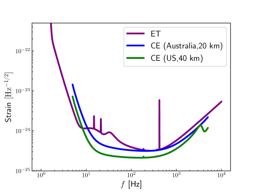
where is the observed chirp mass, is the total mass of a binary system with the component masses and , is the symmetric mass ratio, is the luminosity distance to the GW source, is the gravitational constant, is the speed of light, is the lower cutoff frequency ( Hz for ET and Hz for CE), is the frequency at the last stable orbit with [36], and represents the one-side noise power spectral density (PSD) of the -th GW detector. We wish to note that in this work we consider the waveform in the inspiralling stage for a non-spinning BNS system. Hence, the upper cutoff frequency is chosen as the frequency at the last stable orbit. If the inspiral-merger-ringdown waveform is considered, a higher SNR is expected to provide better measurements on , thus providing better constraints on cosmological parameters. We adopt the PSD of ET from ref. [109] and that of CE from ref. [110] (we consider one 40 km-arm-length CE in the US and one 20 km-arm-length CE in Australia and the noise curves are shown in figure 1). characterizes the detector response, where is the inclination angle between the binary’s orbital angular momentum and the line of sight, and are the th detector’s antenna response functions of two GW polarizations, and . Note that we adopt the NS’s mass distribution from the analysis of the latest O3 observation (figure 7 of ref. [111]).
The detector response functions are related to the source location, the polarization angle, the detector’s location (latitude , longitude , the angle between the interferometer arms , and the orientation angle of the detector’s arms measured counter-clockwise from East of the Earth to the bisector of the interferometer arms). In table 1, we list the coordinates of the GW observatories considered in this work. Some other 3G GW detectors’ location candidates could be found in ref. [112]. We note that the 3G GW detectors have much wider frequency range than the current ground-based GW detectors. The time of BNS merger is a function of . Thus, the BNS signals can be found in the 3G GW band for hours, even for several days, and in the 2G GW band for tens of minutes [113]. Therefore, the time dependence in the detector response functions is considered in this work. The forms of and are related to these parameters, as detailedly described in refs. [114, 115, 116].
| GW detector | ||||
|---|---|---|---|---|
| Cosmic Explorer, USA | 90.000 | |||
| Einstein Telescope, Europe | 60.000 | |||
| Cosmic Explorer, Australia | 90.000 |
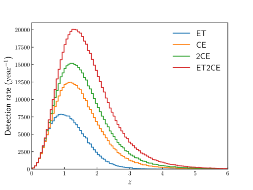
According to our calculation, we obtain the numbers of the GW events detected by ET (545763), CE (1017618), the 2CE network (1317183), and the ET2CE network (1815501), assuming a three-year observation. We see that the number of GW events detected by CE is more than twice of ET. Compared to the single CE observatory, the number of GW events detected by the 2CE network almost doubles. Meanwhile, the number of GW events detected by the ET2CE network is slightly more than that of the 2CE network. In figure 2, we show the expected detection rate as a function of redshift for ET, CE, 2CE, and ET2CE.
2.3 GW dark sirens
Under the stationary phase approximation [121], the Fourier transform of the time-domain waveform for a detector network (with detectors) is given by [113]
| (2.4) |
with given by
| (2.5) |
where is the diagonal matrix with , n is the propagation direction of a GW, and is the location of the th detector. Here is PSD of the -th detector. We consider the waveform in the inspiralling stage for a non-spinning BNS system. We adopt the restricted Post-Newtonian (PN) approximation and calculate the waveform to the 3.5PN order [122, 123],
| (2.6) |
where the Fourier amplitude is given by
| (2.7) |
Here is the coalescence phase and the detailed forms of and can be found in refs. [122, 123]. Note that we employ the stationary phase approximation to obtain the frequency-domain expression of GW waveform, in which the time in , , and is replaced by [124, 113], with the coalescence time.
The tidal contribution to the GW phase from a BNS system is given by [94]
| (2.8) |
where the sum is comprised of the components of the binary system, , and is the tidal deformation, which is related to the EoS of NS and characterizes changes of the quadruple of NS. It is comparable in magnitude with the 3.5PN phasing term for NSs [94]. Due to the fact that EoS of NS is still unknown, we choose SLy [125] as the fiducial EoS of NS that is also consistent with the current observation [126]. In fact, the consideration of different EoSs of NS may lead to different constraint results. In ref. [94], Messenger and Read found that for the three typical NS’s EoSs, the redshift measurement errors obtained by using the tidal measurement method can differ by several times (a stiffer EoS gives better redshift measurement). In ref. [96], Wang et al. used different EoSs of NS and focused on constraining dark energy by fixing other cosmological parameters (a stiffer EoS of NS gives better constraints). Hence, in this work, in order to make the cosmological analysis representative, we choose a medium EoS of NS, namely SLy.
In this work, following ref. [96], in order to parameterize the EoS of NS, we express the – relation as a linear function of the NS mass in the range of as
| (2.9) |
where and are tidal effect parameters. For the fitting of SLy, we obtain and , where the goodness-of-fit value is 0.999. Therefore, the influence of the fitting errors on the results is almost negligible.
Then we can use the Fisher information matrix to calculate the measurement errors of the GW parameters. For a set of parameters , the Fisher information matrix of a network including independent GW detectors is given by
| (2.10) |
where denotes twelve parameters (, , , , , , , , , , , ) for a given BNS system. The inner product is defined as
| (2.11) |
where represents complex conjugate. Here we numerically calculate the partial derivatives by , with . In order to verify the robustness of our code, we compare our Fisher matrix with that obtained from the state-of-the-art code [127]. We find that the results are consistent after optimizing the value of to ensure the convergence of the derivative. The Fisher information matrix can then be used to calculate the measurement errors of the GW parameters
| (2.12) |
The instrumental error is . The measurement of is also affected by the weak lensing and we adopt the form [128, 129, 130]
| (2.13) |
The total error of is given by
| (2.14) |
Throughout this work, we simulate the BNS mergers with random binary orientations and sky directions. The sky direction, binary inclination, polarization angle, and the coalescence phase are randomly chosen in the ranges of , , , , and . For the NS’s mass, we adopt the mass distribution based on the analysis of the latest O3 observation (figure 7 of ref. [111]). Without loss of generality, the merger time is chosen to in our analysis. The simulated GW dark sirens satisfy the redshift distributions corresponding to ET, CE, 2CE, and ET2CE shown in figure 2.
When using BNS tidal deformation measurements to obtain redshift information, the GW tidal phases need to be precisely measured to obtain the source-frame mass information (related to and ). Combining with the observed chirp mass information obtained from the measurements of observed GW frequency and its time derivative , the redshift information could be obtained by breaking the parameter degeneracies between mass and redshift. In our analysis, we consider the correlation between the twelve parameters to calculate the measurement errors of redshifts. Using eq. (2.12), we can obtain the measurement errors of redshifts, .
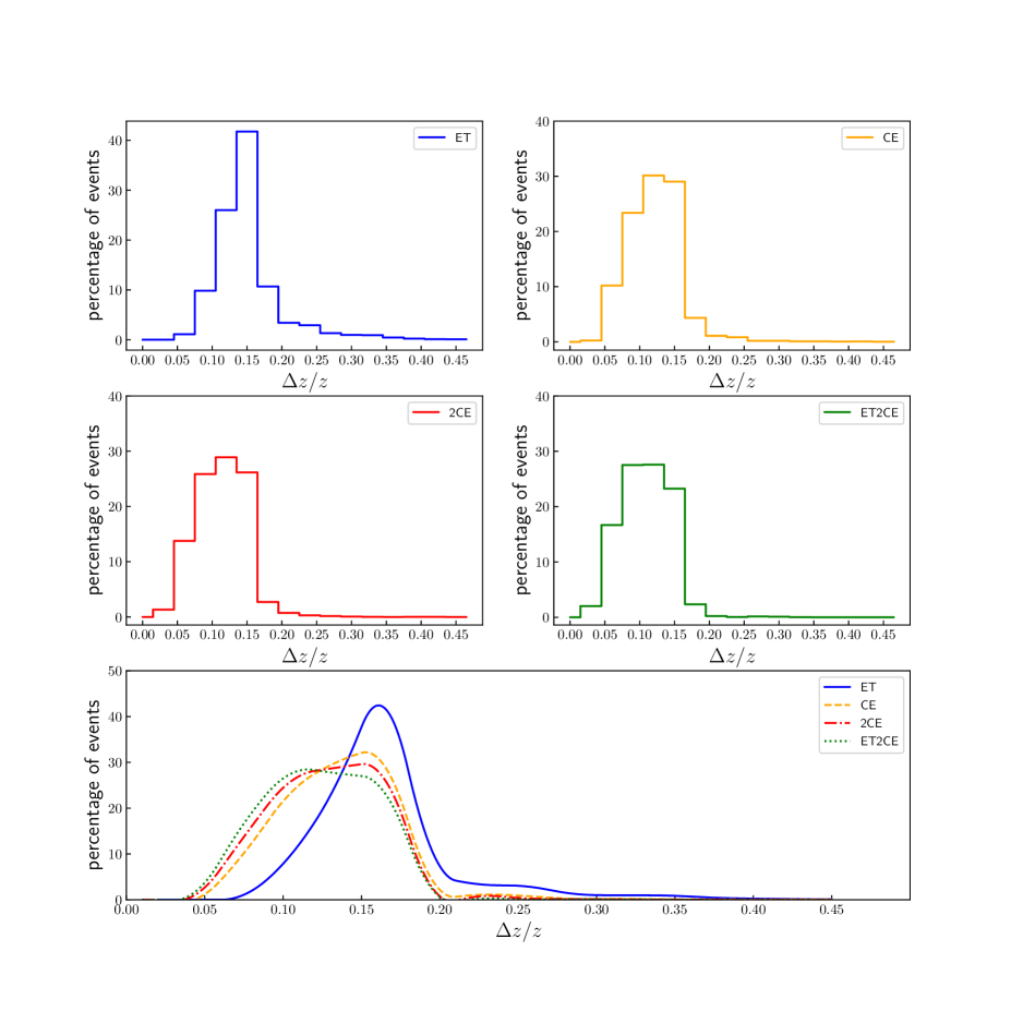
In the upper and middle panels of figure 3, we show the distributions of for ET, CE, 2CE, and ET2CE. In order to be more intuitive, in the lower panel of figure 3, we use the interpolation method to fit the histograms above. We see that the measurement precisions of redshifts are mainly –. ET2CE gives the best redshift measurement, followed by 2CE, CE, and ET. The ET case shows evident difference compared with the other three cases, while the CE, 2CE, and ET2CE cases also have some slight differences.
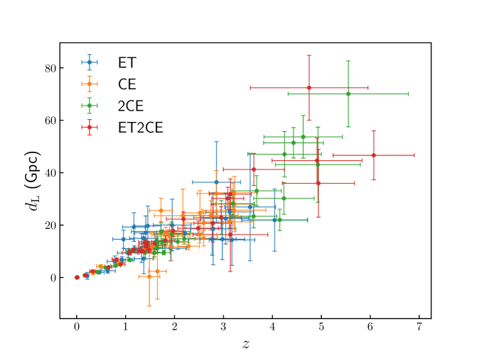
In figure 4, we show the simulated GW standard sirens observed by ET, CE, 2CE, and ET2CE. For simplicity, we show only 30 data points for each observation. To account for fluctuations in the measured values resulting from actual observations, we represent the standard siren data points with Gaussian randomization. Specifically, the central value is populated according to a Gaussian distribution with mean equal to the fiducial value and standard deviation equal to the measurement error.
2.4 Method of constraining cosmological parameters
Given a set of GW data , the posterior probability distribution of the cosmological parameters is
| (2.15) |
where is the prior on cosmological parameters . The likelihood function for the GW data is given by
| (2.16) |
where represents the -th GW event, and are two Gaussian distributions with the standard deviations calculated from eq. (2.12), and is the redshift prior that is assumed to be uniform for simplicity. For the dark siren method, the redshifts of the GW events are not precisely measured. Therefore, the redshift should be marginalized out to obtain the constraints on cosmological parameters, i.e., eq. (2.16) should be rewritten as
| (2.17) |
Note that in the above equation is not explicitly shown because it is assumed to be a constant.
Here, we also note that the method described above is valid under two assumptions: (i) the measurements of and are assumed to be nearly independent, with measured from the GW amplitude and measured from the GW phase, and (ii) the detection probability (selection bias) does not depend on the observed values of and . In a more realistic approach, the observed values of and may deviate from the simulated values. In such cases, it is necessary to use the observed data to calculate SNRs and the detection probability. If assumption (ii) is not satisfied, the Bayesian inference could be corrected by adding the redshift prior conditioned on detection, which is basically the detection rate as a function of redshift (see ref. [131] for an example).
Model Parameter ET CE 2CE ET2CE CDM CDM
3 Results
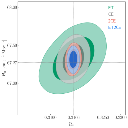
We use the simulated GW dark siren data from ET, CE, 2CE, and ET2CE and by performing the MCMC analysis [132] we use the mock data of dark sirens to constrain the CDM and CDM models. The constraint results are shown in figures 5 and 6 and summarized in table 2. For a parameter , we use and to represent its absolute (1) and relative errors, respectively, with defined as .
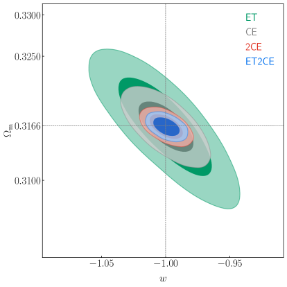
We first take a look at the CDM model. In the left panel of figure 5, we show the constraints in the – plane. We can clearly see that GWs place quite tight constraints on the parameters. Owing to the fact that the detection sensitivity of CE is better than that of ET, ET shows the worst constraint results among the four cases. However, even so, ET gives , , and which are comparable with the results of , , and by the latest Planck TT,TE,EE+lowE+BAO+Pantheon data [32]. Meanwhile, ET and CE show positive correlation between and , while there is almost no correlation between and when using the mock GW dark siren data of 2CE and ET2CE. However, the obvious anti-correlation is obtained when using the traditional EM cosmological probes. In the right panel of figure 5, we show the constraints in the – plane. We find that the 2CE network can give quite tight constraints on the cosmological parameters with the constraint precisions of , , and being , , and , respectively. So, even for the EoS of dark energy, the standard of precision cosmology is nearly achieved. Furthermore, we find that using the ET2CE mock data, the constraint precisions of , , and are , , and , respectively, all meeting the standard of precision cosmology.
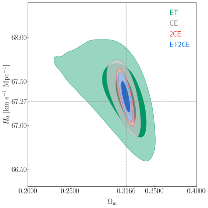
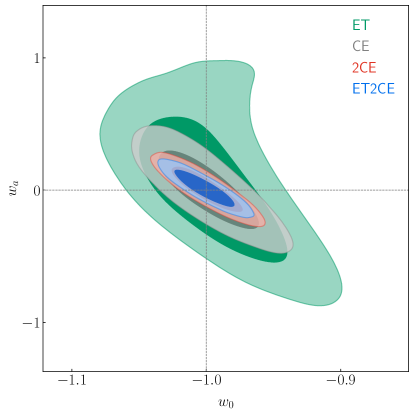
In figure 6, we show the constraint results of the CDM model. Among the four cases, ET gives the worst constraint results. CE gives much better constraints than ET. 2CE gives similar constraint results with ET2CE. Quantitatively, ET gives and , comparable with the results of and by the latest Planck TT,TE,EE+lowE+BAO+Pantheon data [32]. Meanwhile, the constraint results of ET are also basically consistent with those given in ref. [95]. For the case of using CE, the constraint results are much better than those of ET, also better than those of the latest Planck TT,TE,EE+lowE+BAO+Pantheon data. What’s more, when considering 2CE and ET2CE, the constraint precisions of are (2CE) and (ET2CE). For , ET2CE gives .
4 Discussion
In section 3, we compare the constraint results of the GW dark sirens (tidal measurements) with the current cosmological observations, from which the potential of the GW dark sirens can be clearly seen. Since third-generation GW detectors will begin observation in the 2030s, it is also necessary to show the comparisons with other cosmological observations in the same period.
4.1 Comparison with future other GW standard siren observations
In the 3G GW detector network era, lots of bright sirens could also be used to study the cosmic expansion history. Belgacem et al. [90] used the mock bright siren data (based on the 10-year observation of ET2CE and THESEUS) to measure dark energy and obtained for the optimistic case of observing EM counterparts. When combining the mock bright siren data of ET2CE with the current CMB+BAO+SN data, the constraint errors could be reduced to that is comparable with the constraint results of 2CE in this work. For the case of the CDM model, the combination of the mock bright siren data and the CMB+BAO+SN data gives and [90] that are also comparable with those of 2CE in this work.
In the same period of the 3G GW detectors, the space-based GW detectors will begin detecting GWs generated by the massive or supermassive black hole binaries (SMBHBs). Wang et al. [50] used the mock bright siren data of the LISA-Taiji network to measure dark energy. Zhu et al. [133] used the mock bright siren data of LISA-TianQin network to measure dark energy. However, owing to the fact that the number of the detectable bright sirens of SMBHBs are small (about ) within 5-year observation, the constraint results are all weaker than those of this work.
4.2 Comparison with future EM surveys
In the next decades, the fourth-generation dark energy surveys will also precisely measure dark energy [134, 135]. Pierel et al. [134] forecasted the ability of cosmological parameter estimation using strongly lensed SN from the Roman Space Telescope (previously WFIRST). The CMB+BAO+SN+UltraDeep lensed SN data give in the CDM model, and and in the CDM model, comparable with those of 2CE in this work. Recently, Euclid Collaboration [135] forecasted the constraint results of Euclid. The pessimistic case of Euclid (see ref. [135] for more details) gives and that are comparable with those of 2CE. If considering the combination of CMB-S4 and Euclid (pessimistic), the constraint results are worse than those of ET2CE. While considering the optimistic case of Euclid (see ref. [135] for more details), the absolute errors are reduced to and that are comparable with those of ET2CE. If considering the combination of CMB-S4 and Euclid (optimistic), the constraint results are also comparable with those of ET2CE.
4.3 Comparison with future other cosmological probes
In the future, neutral hydrogen 21 cm intensity mapping (IM) will become an important tool to explore the nature of dark energy [136, 137, 138, 139, 140, 141, 142]. Bull et al. [136] obtained and by using the SKA1-MID+MeerKAT data, which are comparable with those of 2CE. Xu et al. [137] obtained and by using the full-scale Tianlai data, which are comparable with those of ET. Wu et al. [56] forecasted cosmological parameters using the combination of four promising cosmological probes, 21 cm IM, GW, fast radio burst, and strong gravitational lensing, and obtained , comparable with that of CE.
5 Conclusion
In the next decades, the third-generation GW detectors will detect large amounts of ( per year) GW events generated by the BNS mergers. By measuring the additional tidal deformation-phase term, the redshifts of the GW sources could be obtained. Hence, the cosmic expansion history can be investigated using solely GW observations. In this work, based on the three-year observation, we simulate such GW dark sirens of ET, CE, 2CE, and ET2CE to perform cosmological analysis. Note that the assumption of the EoS of NS being perfectly known is adopted in this work. We wish to investigate whether the Hubble constant and the EoS of dark energy can both be precisely measured using only GW dark sirens detected by the 3G GW observations.
We find that ET gives the worst constraints among the four cases. Even so, ET gives that is comparable with the latest constraint result of Planck TT,TE,EE+lowE+ BAO + Pantheon. Meanwhile, the constraint precision of using the mock 2CE data is close to , which almost meets the standard of precision cosmology. The 3G GW detector network has a strong capability to constrain the EoS parameter of dark energy , with a precision of 0.95%. For the Hubble constant, the single ET observatory gives quite tight constraint with the precision being . Using the ET2CE network, we obtain the constraint precision of being .
We also discuss the case of the two-parameter dark-energy model. We find that ET gives comparable constraint results with those of the latest Planck TT,TE,EE+lowE+ BAO + Pantheon data. CE gives much better constraint results than those of ET. ET2CE gives slightly better constraint results than 2CE. Using ET2CE, we obtain the constraint precision of being . Moreover, ET2CE gives that is much better than the result of the latest Planck TT,TE,EE+lowE+BAO+Pantheon data.
In addition, we discuss the comparison of the constraint results of GW dark sirens (tidal measurements) with those of the same-period other cosmological observations. We find that GW dark sirens show strong ability to measure the Hubble constant and dark energy. The constraints on the Hubble constant and the EoS of dark energy using GW dark sirens of ET2CE are comparable with those of the combination of the fourth-generation dark energy surveys (optimistic case of Euclid) and CMB-S4.
Our results show that the precision cosmology can be achieved by solely using the GW dark sirens observed by the 3G GW detectors. It can be expected that the 3G GW detectors would play a key role in helping solve the Hubble tension and reveal the fundamental nature of dark energy.
Acknowledgments
We thank Ji-Yu Song, Jiming Yu, Liang-Gui Zhu, Arnab Dhani, Ssohrab Borhanian, Peng-Ju Wu, Ling-Feng Wang, Tao Han, Jing-Zhao Qi, Bo Wang, and Rui-Qi Zhu for helpful discussions. This work was supported by the National SKA Program of China (Grants Nos. 2022SKA0110200 and 2022SKA0110203), the National Natural Science Foundation of China (Grants Nos. 11975072, 11875102, and 11835009), and the 111 Project (Grant No. B16009).
References
- [1] A.R. Sandage, Cosmology: A Search for Two Numbers, Physics Today 23 (1970) 34.
- [2] Supernova Search Team collaboration, Observational evidence from supernovae for an accelerating universe and a cosmological constant, Astron. J. 116 (1998) 1009 [astro-ph/9805201].
- [3] Supernova Cosmology Project collaboration, Measurements of and from 42 high redshift supernovae, Astrophys. J. 517 (1999) 565 [astro-ph/9812133].
- [4] Planck collaboration, Planck 2018 results. VI. Cosmological parameters, Astron. Astrophys. 641 (2020) A6 [1807.06209].
- [5] A.G. Riess et al., A Comprehensive Measurement of the Local Value of the Hubble Constant with 1 km s-1 Mpc-1 Uncertainty from the Hubble Space Telescope and the SH0ES Team, Astrophys. J. Lett. 934 (2022) L7 [2112.04510].
- [6] A.G. Riess, The Expansion of the Universe is Faster than Expected, Nature Rev. Phys. 2 (2019) 10 [2001.03624].
- [7] L. Verde, T. Treu and A.G. Riess, Tensions between the Early and the Late Universe, Nature Astron. 3 (2019) 891 [1907.10625].
- [8] R.-Y. Guo, J.-F. Zhang and X. Zhang, Can the tension be resolved in extensions to CDM cosmology?, JCAP 02 (2019) 054 [1809.02340].
- [9] L.-Y. Gao, Z.-W. Zhao, S.-S. Xue and X. Zhang, Relieving the H 0 tension with a new interacting dark energy model, JCAP 07 (2021) 005 [2101.10714].
- [10] E. Di Valentino, O. Mena, S. Pan, L. Visinelli, W. Yang, A. Melchiorri et al., In the realm of the Hubble tension—a review of solutions, Class. Quant. Grav. 38 (2021) 153001 [2103.01183].
- [11] E. Abdalla et al., Cosmology intertwined: A review of the particle physics, astrophysics, and cosmology associated with the cosmological tensions and anomalies, JHEAp 34 (2022) 49 [2203.06142].
- [12] R.-G. Cai, Editorial, Sci. China Phys. Mech. Astron. 63 (2020) 290401.
- [13] R.-G. Cai, Z.-K. Guo, L. Li, S.-J. Wang and W.-W. Yu, Chameleon dark energy can resolve the Hubble tension, Phys. Rev. D 103 (2021) 121302 [2102.02020].
- [14] W. Yang, S. Pan, E. Di Valentino, R.C. Nunes, S. Vagnozzi and D.F. Mota, Tale of stable interacting dark energy, observational signatures, and the tension, JCAP 09 (2018) 019 [1805.08252].
- [15] E. Di Valentino, A. Melchiorri, O. Mena and S. Vagnozzi, Nonminimal dark sector physics and cosmological tensions, Phys. Rev. D 101 (2020) 063502 [1910.09853].
- [16] E. Di Valentino, A. Melchiorri, O. Mena and S. Vagnozzi, Interacting dark energy in the early 2020s: A promising solution to the and cosmic shear tensions, Phys. Dark Univ. 30 (2020) 100666 [1908.04281].
- [17] E. Di Valentino et al., Snowmass2021 - Letter of interest cosmology intertwined II: The hubble constant tension, Astropart. Phys. 131 (2021) 102605 [2008.11284].
- [18] M. Liu, Z. Huang, X. Luo, H. Miao, N.K. Singh and L. Huang, Can Non-standard Recombination Resolve the Hubble Tension?, Sci. China Phys. Mech. Astron. 63 (2020) 290405 [1912.00190].
- [19] X. Zhang and Q.-G. Huang, Measuring H0 from low-z datasets, Sci. China Phys. Mech. Astron. 63 (2020) 290402 [1911.09439].
- [20] Q. Ding, T. Nakama and Y. Wang, A gigaparsec-scale local void and the Hubble tension, Sci. China Phys. Mech. Astron. 63 (2020) 290403 [1912.12600].
- [21] H. Li and X. Zhang, A novel method of measuring cosmological distances using broad-line regions of quasars, Sci. Bull. 65 (2020) 1419 [2005.10458].
- [22] L.-F. Wang, J.-H. Zhang, D.-Z. He, J.-F. Zhang and X. Zhang, Constraints on interacting dark energy models from time-delay cosmography with seven lensed quasars, Mon. Not. Roy. Astron. Soc. 514 (2022) 1433 [2102.09331].
- [23] S. Vagnozzi, F. Pacucci and A. Loeb, Implications for the Hubble tension from the ages of the oldest astrophysical objects, JHEAp 36 (2022) 27 [2105.10421].
- [24] S. Vagnozzi, Consistency tests of CDM from the early integrated Sachs-Wolfe effect: Implications for early-time new physics and the Hubble tension, Phys. Rev. D 104 (2021) 063524 [2105.10425].
- [25] R.-Y. Guo, J.-F. Zhang and X. Zhang, Inflation model selection revisited after a 1.91% measurement of the Hubble constant, Sci. China Phys. Mech. Astron. 63 (2020) 290406 [1910.13944].
- [26] S. Vagnozzi, New physics in light of the tension: An alternative view, Phys. Rev. D 102 (2020) 023518 [1907.07569].
- [27] L. Feng, D.-Z. He, H.-L. Li, J.-F. Zhang and X. Zhang, Constraints on active and sterile neutrinos in an interacting dark energy cosmology, Sci. China Phys. Mech. Astron. 63 (2020) 290404 [1910.03872].
- [28] M.-X. Lin, W. Hu and M. Raveri, Testing in Acoustic Dark Energy with Planck and ACT Polarization, Phys. Rev. D 102 (2020) 123523 [2009.08974].
- [29] A. Hryczuk and K. Jodłowski, Self-interacting dark matter from late decays and the tension, Phys. Rev. D 102 (2020) 043024 [2006.16139].
- [30] L.-Y. Gao, S.-S. Xue and X. Zhang, Dark energy and matter interacting scenario can relieve and tensions, 2212.13146.
- [31] Z.-W. Zhao, J.-G. Zhang, Y. Li, J.-M. Zou, J.-F. Zhang and X. Zhang, First statistical measurement of the Hubble constant using unlocalized fast radio bursts, 2212.13433.
- [32] D. Brout et al., The Pantheon+ Analysis: Cosmological Constraints, Astrophys. J. 938 (2022) 110 [2202.04077].
- [33] D.E. Holz and S.A. Hughes, Using gravitational-wave standard sirens, Astrophys. J. 629 (2005) 15 [astro-ph/0504616].
- [34] N. Dalal, D.E. Holz, S.A. Hughes and B. Jain, Short grb and binary black hole standard sirens as a probe of dark energy, Phys. Rev. D 74 (2006) 063006 [astro-ph/0601275].
- [35] C. Cutler and D.E. Holz, Ultra-high precision cosmology from gravitational waves, Phys. Rev. D 80 (2009) 104009 [0906.3752].
- [36] W. Zhao, C. Van Den Broeck, D. Baskaran and T.G.F. Li, Determination of Dark Energy by the Einstein Telescope: Comparing with CMB, BAO and SNIa Observations, Phys. Rev. D 83 (2011) 023005 [1009.0206].
- [37] R.-G. Cai and T. Yang, Estimating cosmological parameters by the simulated data of gravitational waves from the Einstein Telescope, Phys. Rev. D 95 (2017) 044024 [1608.08008].
- [38] R.-G. Cai, T.-B. Liu, X.-W. Liu, S.-J. Wang and T. Yang, Probing cosmic anisotropy with gravitational waves as standard sirens, Phys. Rev. D 97 (2018) 103005 [1712.00952].
- [39] R.-G. Cai and T. Yang, Standard sirens and dark sector with Gaussian process, EPJ Web Conf. 168 (2018) 01008 [1709.00837].
- [40] X. Zhang, Gravitational wave standard sirens and cosmological parameter measurement, Sci. China Phys. Mech. Astron. 62 (2019) 110431 [1905.11122].
- [41] W. Zhao, B.S. Wright and B. Li, Constraining the time variation of Newton’s constant with gravitational-wave standard sirens and supernovae, JCAP 10 (2018) 052 [1804.03066].
- [42] M. Du, W. Yang, L. Xu, S. Pan and D.F. Mota, Future constraints on dynamical dark-energy using gravitational-wave standard sirens, Phys. Rev. D 100 (2019) 043535 [1812.01440].
- [43] Y.-F. Cai, C. Li, E.N. Saridakis and L. Xue, gravity after GW170817 and GRB170817A, Phys. Rev. D 97 (2018) 103513 [1801.05827].
- [44] W. Yang, S. Pan, E. Di Valentino, B. Wang and A. Wang, Forecasting interacting vacuum-energy models using gravitational waves, JCAP 05 (2020) 050 [1904.11980].
- [45] W. Yang, S. Vagnozzi, E. Di Valentino, R.C. Nunes, S. Pan and D.F. Mota, Listening to the sound of dark sector interactions with gravitational wave standard sirens, JCAP 07 (2019) 037 [1905.08286].
- [46] R.R.A. Bachega, A.A. Costa, E. Abdalla and K.S.F. Fornazier, Forecasting the Interaction in Dark Matter-Dark Energy Models with Standard Sirens From the Einstein Telescope, JCAP 05 (2020) 021 [1906.08909].
- [47] Z. Chang, Q.-G. Huang, S. Wang and Z.-C. Zhao, Low-redshift constraints on the Hubble constant from the baryon acoustic oscillation “standard rulers” and the gravitational wave “standard sirens”, Eur. Phys. J. C 79 (2019) 177.
- [48] J.-h. He, Accurate method to determine the systematics due to the peculiar velocities of galaxies in measuring the Hubble constant from gravitational-wave standard sirens, Phys. Rev. D 100 (2019) 023527 [1903.11254].
- [49] Z.-W. Zhao, L.-F. Wang, J.-F. Zhang and X. Zhang, Prospects for improving cosmological parameter estimation with gravitational-wave standard sirens from Taiji, Sci. Bull. 65 (2020) 1340 [1912.11629].
- [50] L.-F. Wang, S.-J. Jin, J.-F. Zhang and X. Zhang, Forecast for cosmological parameter estimation with gravitational-wave standard sirens from the LISA-Taiji network, Sci. China Phys. Mech. Astron. 65 (2022) 210411 [2101.11882].
- [51] J.-Z. Qi, S.-J. Jin, X.-L. Fan, J.-F. Zhang and X. Zhang, Using a multi-messenger and multi-wavelength observational strategy to probe the nature of dark energy through direct measurements of cosmic expansion history, JCAP 12 (2021) 042 [2102.01292].
- [52] S.-J. Jin, L.-F. Wang, P.-J. Wu, J.-F. Zhang and X. Zhang, How can gravitational-wave standard sirens and 21-cm intensity mapping jointly provide a precise late-universe cosmological probe?, Phys. Rev. D 104 (2021) 103507 [2106.01859].
- [53] L.-G. Zhu, L.-H. Xie, Y.-M. Hu, S. Liu, E.-K. Li, N.R. Napolitano et al., Constraining the Hubble constant to a precision of about 1% using multi-band dark standard siren detections, Sci. China Phys. Mech. Astron. 65 (2022) 259811 [2110.05224].
- [54] J.M.S. de Souza, R. Sturani and J. Alcaniz, Cosmography with standard sirens from the Einstein Telescope, JCAP 03 (2022) 025 [2110.13316].
- [55] L.-F. Wang, Y. Shao, G.-P. Zhang, J.-F. Zhang and X. Zhang, Ultra-low-frequency gravitational waves from individual supermassive black hole binaries as standard sirens, 2201.00607.
- [56] P.-J. Wu, Y. Shao, S.-J. Jin and X. Zhang, A path to precision cosmology: synergy between four promising late-universe cosmological probes, JCAP 06 (2023) 052 [2202.09726].
- [57] S.-J. Jin, R.-Q. Zhu, L.-F. Wang, H.-L. Li, J.-F. Zhang and X. Zhang, Impacts of gravitational-wave standard siren observations from Einstein Telescope and Cosmic Explorer on weighing neutrinos in interacting dark energy models, Commun. Theor. Phys. 74 (2022) 105404 [2204.04689].
- [58] J.-Y. Song, L.-F. Wang, Y. Li, Z.-W. Zhao, J.-F. Zhang, W. Zhao et al., Synergy between CSST galaxy survey and gravitational-wave observation: Inferring the Hubble constant from dark standard sirens, 2212.00531.
- [59] W.-T. Hou, J.-Z. Qi, T. Han, J.-F. Zhang, S. Cao and X. Zhang, Prospects for constraining interacting dark energy models from gravitational wave and gamma ray burst joint observation, JCAP 05 (2023) 017 [2211.10087].
- [60] H.-Y. Chen, Systematic Uncertainty of Standard Sirens from the Viewing Angle of Binary Neutron Star Inspirals, Phys. Rev. Lett. 125 (2020) 201301 [2006.02779].
- [61] R. Gray et al., Cosmological inference using gravitational wave standard sirens: A mock data analysis, Phys. Rev. D 101 (2020) 122001 [1908.06050].
- [62] M. Califano, I. de Martino, D. Vernieri and S. Capozziello, Exploiting the Einstein Telescope to solve the Hubble tension, 2208.13999.
- [63] Y.-J. Wang, J.-Z. Qi, B. Wang, J.-F. Zhang, J.-L. Cui and X. Zhang, Cosmological model-independent measurement of cosmic curvature using distance sum rule with the help of gravitational waves, Mon. Not. Roy. Astron. Soc. 516 (2022) 5187 [2201.12553].
- [64] A. Dhani, S. Borhanian, A. Gupta and B. Sathyaprakash, Cosmography with bright and Love sirens, 2212.13183.
- [65] E.O. Colgáin, Probing the Anisotropic Universe with Gravitational Waves, in 17th Italian-Korean Symposium on Relativistic Astrophysics, 3, 2022 [2203.03956].
- [66] M.-D. Cao, J. Zheng, J.-Z. Qi, X. Zhang and Z.-H. Zhu, A New Way to Explore Cosmological Tensions Using Gravitational Waves and Strong Gravitational Lensing, Astrophys. J. 934 (2022) 108 [2112.14564].
- [67] H. Leandro, V. Marra and R. Sturani, Measuring the Hubble constant with black sirens, Phys. Rev. D 105 (2022) 023523 [2109.07537].
- [68] C. Ye and M. Fishbach, Cosmology with standard sirens at cosmic noon, Phys. Rev. D 104 (2021) 043507 [2103.14038].
- [69] H.-Y. Chen, P.S. Cowperthwaite, B.D. Metzger and E. Berger, A Program for Multimessenger Standard Siren Cosmology in the Era of LIGO A+, Rubin Observatory, and Beyond, Astrophys. J. Lett. 908 (2021) L4 [2011.01211].
- [70] A. Mitra, J. Mifsud, D.F. Mota and D. Parkinson, Cosmology with the Einstein Telescope: No Slip Gravity Model and Redshift Specifications, Mon. Not. Roy. Astron. Soc. 502 (2021) 5563 [2010.00189].
- [71] N.B. Hogg, M. Martinelli and S. Nesseris, Constraints on the distance duality relation with standard sirens, JCAP 12 (2020) 019 [2007.14335].
- [72] R.C. Nunes, Searching for modified gravity in the astrophysical gravitational wave background: Application to ground-based interferometers, Phys. Rev. D 102 (2020) 024071 [2007.07750].
- [73] S. Borhanian, A. Dhani, A. Gupta, K.G. Arun and B.S. Sathyaprakash, Dark Sirens to Resolve the Hubble–Lemaître Tension, Astrophys. J. Lett. 905 (2020) L28 [2007.02883].
- [74] S.-J. Jin, S.-S. Xing, Y. Shao, J.-F. Zhang and X. Zhang, Joint constraints on cosmological parameters using future multi-band gravitational wave standard siren observations*, Chin. Phys. C 47 (2023) 065104 [2301.06722].
- [75] S.-J. Jin, Y.-Z. Zhang, J.-Y. Song, J.-F. Zhang and X. Zhang, The Taiji-TianQin-LISA network: Precisely measuring the Hubble constant using both bright and dark sirens, 2305.19714.
- [76] L. Bian et al., The Gravitational-Wave Physics II: Progress, Sci. China Phys. Mech. Astron. 64 (2021) 120401 [2106.10235].
- [77] B.F. Schutz, Determining the Hubble Constant from Gravitational Wave Observations, Nature 323 (1986) 310.
- [78] L.-X. Li and B. Paczynski, Transient events from neutron star mergers, Astrophys. J. Lett. 507 (1998) L59 [astro-ph/9807272].
- [79] E. Nakar, Short-Hard Gamma-Ray Bursts, Phys. Rept. 442 (2007) 166 [astro-ph/0701748].
- [80] LIGO Scientific, Virgo, 1M2H, Dark Energy Camera GW-E, DES, DLT40, Las Cumbres Observatory, VINROUGE, MASTER collaboration, A gravitational-wave standard siren measurement of the Hubble constant, Nature 551 (2017) 85 [1710.05835].
- [81] LIGO Scientific, Virgo collaboration, GWTC-1: A Gravitational-Wave Transient Catalog of Compact Binary Mergers Observed by LIGO and Virgo during the First and Second Observing Runs, Phys. Rev. X 9 (2019) 031040 [1811.12907].
- [82] LIGO Scientific, Virgo collaboration, GWTC-2: Compact Binary Coalescences Observed by LIGO and Virgo During the First Half of the Third Observing Run, Phys. Rev. X 11 (2021) 021053 [2010.14527].
- [83] LIGO Scientific, VIRGO, KAGRA collaboration, GWTC-3: Compact Binary Coalescences Observed by LIGO and Virgo During the Second Part of the Third Observing Run, 2111.03606.
- [84] KAGRA, LIGO Scientific, Virgo, VIRGO collaboration, Prospects for observing and localizing gravitational-wave transients with Advanced LIGO, Advanced Virgo and KAGRA, Living Rev. Rel. 23 (2020) 3 [1304.0670].
- [85] H.-Y. Chen, M. Fishbach and D.E. Holz, A two per cent Hubble constant measurement from standard sirens within five years, Nature 562 (2018) 545 [1712.06531].
- [86] LIGO Scientific collaboration, Exploring the Sensitivity of Next Generation Gravitational Wave Detectors, Class. Quant. Grav. 34 (2017) 044001 [1607.08697].
- [87] M. Punturo et al., The Einstein Telescope: A third-generation gravitational wave observatory, Class. Quant. Grav. 27 (2010) 194002.
- [88] M. Evans et al., A Horizon Study for Cosmic Explorer: Science, Observatories, and Community, 2109.09882.
- [89] M. Safarzadeh, E. Berger, K.K.Y. Ng, H.-Y. Chen, S. Vitale, C. Whittle et al., Measuring the delay time distribution of binary neutron stars. II. Using the redshift distribution from third-generation gravitational wave detectors network, Astrophys. J. Lett. 878 (2019) L13 [1904.10976].
- [90] E. Belgacem, Y. Dirian, S. Foffa, E.J. Howell, M. Maggiore and T. Regimbau, Cosmology and dark energy from joint gravitational wave-GRB observations, JCAP 08 (2019) 015 [1907.01487].
- [91] J. Yu, H. Song, S. Ai, H. Gao, F. Wang, Y. Wang et al., Multimessenger Detection Rates and Distributions of Binary Neutron Star Mergers and Their Cosmological Implications, Astrophys. J. 916 (2021) 54 [2104.12374].
- [92] J.-F. Zhang, M. Zhang, S.-J. Jin, J.-Z. Qi and X. Zhang, Cosmological parameter estimation with future gravitational wave standard siren observation from the Einstein Telescope, JCAP 09 (2019) 068 [1907.03238].
- [93] S.-J. Jin, D.-Z. He, Y. Xu, J.-F. Zhang and X. Zhang, Forecast for cosmological parameter estimation with gravitational-wave standard siren observation from the Cosmic Explorer, JCAP 03 (2020) 051 [2001.05393].
- [94] C. Messenger and J. Read, Measuring a cosmological distance-redshift relationship using only gravitational wave observations of binary neutron star coalescences, Phys. Rev. Lett. 108 (2012) 091101 [1107.5725].
- [95] W. Del Pozzo, T.G.F. Li and C. Messenger, Cosmological inference using only gravitational wave observations of binary neutron stars, Phys. Rev. D 95 (2017) 043502 [1506.06590].
- [96] B. Wang, Z. Zhu, A. Li and W. Zhao, Comprehensive analysis of the tidal effect in gravitational waves and implication for cosmology, Astrophys. J. Suppl. 250 (2020) 6 [2005.12875].
- [97] D. Chatterjee, A.H.K. R., G. Holder, D.E. Holz, S. Perkins, K. Yagi et al., Cosmology with Love: Measuring the Hubble constant using neutron star universal relations, Phys. Rev. D 104 (2021) 083528 [2106.06589].
- [98] T. Ghosh, B. Biswas and S. Bose, Simultaneous inference of neutron star equation of state and the Hubble constant with a population of merging neutron stars, Phys. Rev. D 106 (2022) 123529 [2203.11756].
- [99] R. Nair, S. Bose and T.D. Saini, Measuring the Hubble constant: Gravitational wave observations meet galaxy clustering, Phys. Rev. D 98 (2018) 023502 [1804.06085].
- [100] DES, LIGO Scientific, Virgo collaboration, First Measurement of the Hubble Constant from a Dark Standard Siren using the Dark Energy Survey Galaxies and the LIGO/Virgo Binary–Black-hole Merger GW170814, Astrophys. J. Lett. 876 (2019) L7 [1901.01540].
- [101] DES collaboration, A statistical standard siren measurement of the Hubble constant from the LIGO/Virgo gravitational wave compact object merger GW190814 and Dark Energy Survey galaxies, Astrophys. J. Lett. 900 (2020) L33 [2006.14961].
- [102] LIGO Scientific, Virgo, VIRGO collaboration, A Gravitational-wave Measurement of the Hubble Constant Following the Second Observing Run of Advanced LIGO and Virgo, Astrophys. J. 909 (2021) 218 [1908.06060].
- [103] J. Yu, Y. Wang, W. Zhao and Y. Lu, Hunting for the host galaxy groups of binary black holes and the application in constraining Hubble constant, Mon. Not. Roy. Astron. Soc. 498 (2020) 1786 [2003.06586].
- [104] LIGO Scientific, Virgo,, KAGRA, VIRGO collaboration, Constraints on the Cosmic Expansion History from GWTC–3, Astrophys. J. 949 (2023) 76 [2111.03604].
- [105] A. Palmese, C.R. Bom, S. Mucesh and W.G. Hartley, A Standard Siren Measurement of the Hubble Constant Using Gravitational-wave Events from the First Three LIGO/Virgo Observing Runs and the DESI Legacy Survey, Astrophys. J. 943 (2023) 56 [2111.06445].
- [106] P. Madau and M. Dickinson, Cosmic Star Formation History, Ann. Rev. Astron. Astrophys. 52 (2014) 415 [1403.0007].
- [107] S. Vitale, W.M. Farr, K. Ng and C.L. Rodriguez, Measuring the star formation rate with gravitational waves from binary black holes, Astrophys. J. Lett. 886 (2019) L1 [1808.00901].
- [108] LIGO Scientific, Virgo collaboration, Population Properties of Compact Objects from the Second LIGO-Virgo Gravitational-Wave Transient Catalog, Astrophys. J. Lett. 913 (2021) L7 [2010.14533].
- [109] https://www.et-gw.eu/index.php/etsensitivities/.
- [110] https://dcc.cosmicexplorer.org/CE-T2000017/public.
- [111] KAGRA, VIRGO, LIGO Scientific collaboration, Population of Merging Compact Binaries Inferred Using Gravitational Waves through GWTC-3, Phys. Rev. X 13 (2023) 011048 [2111.03634].
- [112] S.E. Gossan, E.D. Hall and S.M. Nissanke, Optimizing the Third Generation of Gravitational-wave Observatories for Galactic Astrophysics, Astrophys. J. 926 (2022) 231 [2110.15322].
- [113] W. Zhao and L. Wen, Localization accuracy of compact binary coalescences detected by the third-generation gravitational-wave detectors and implication for cosmology, Phys. Rev. D 97 (2018) 064031 [1710.05325].
- [114] P. Jaranowski, A. Krolak and B.F. Schutz, Data analysis of gravitational - wave signals from spinning neutron stars. 1. The Signal and its detection, Phys. Rev. D 58 (1998) 063001 [gr-qc/9804014].
- [115] N. Arnaud, M. Barsuglia, M.-A. Bizouard, P. Canitrot, F. Cavalier, M. Davier et al., Detection in coincidence of gravitational wave bursts with a network of interferometric detectors. 1. Geometric acceptance and timing, Phys. Rev. D 65 (2002) 042004 [gr-qc/0107081].
- [116] B.F. Schutz, Networks of gravitational wave detectors and three figures of merit, Class. Quant. Grav. 28 (2011) 125023 [1102.5421].
- [117] LIGO Scientific Collaboration, “LIGO Algorithm Library - LALSuite.” free software (GPL), 2018. 10.7935/GT1W-FZ16.
- [118] G. Ashton et al., BILBY: A user-friendly Bayesian inference library for gravitational-wave astronomy, Astrophys. J. Suppl. 241 (2019) 27 [1811.02042].
- [119] M. Di Giovanni, C. Giunchi, G. Saccorotti, A. Berbellini, L. Boschi, M. Olivieri et al., A seismological study of the sos enattos area—the sardinia candidate site for the einstein telescope, Seismological Society of America 92 (2021) 352.
- [120] S. Borhanian, GWBENCH: a novel Fisher information package for gravitational-wave benchmarking, Class. Quant. Grav. 38 (2021) 175014 [2010.15202].
- [121] X. Zhang, T. Liu and W. Zhao, Gravitational radiation from compact binary systems in screened modified gravity, Phys. Rev. D 95 (2017) 104027 [1702.08752].
- [122] B.S. Sathyaprakash and B.F. Schutz, Physics, Astrophysics and Cosmology with Gravitational Waves, Living Rev. Rel. 12 (2009) 2 [0903.0338].
- [123] L. Blanchet and B.R. Iyer, Hadamard regularization of the third post-Newtonian gravitational wave generation of two point masses, Phys. Rev. D 71 (2005) 024004 [gr-qc/0409094].
- [124] M. Maggiore, Gravitational Waves. Vol. 1: Theory and Experiments, Oxford Master Series in Physics, Oxford University Press (2007).
- [125] F. Douchin and P. Haensel, A unified equation of state of dense matter and neutron star structure, Astron. Astrophys. 380 (2001) 151 [astro-ph/0111092].
- [126] LIGO Scientific, Virgo collaboration, GW170817: Observation of Gravitational Waves from a Binary Neutron Star Inspiral, Phys. Rev. Lett. 119 (2017) 161101 [1710.05832].
- [127] F. Iacovelli, M. Mancarella, S. Foffa and M. Maggiore, GWFAST: A Fisher Information Matrix Python Code for Third-generation Gravitational-wave Detectors, Astrophys. J. Supp. 263 (2022) 2 [2207.06910].
- [128] N. Tamanini, C. Caprini, E. Barausse, A. Sesana, A. Klein and A. Petiteau, Science with the space-based interferometer eLISA. III: Probing the expansion of the Universe using gravitational wave standard sirens, JCAP 04 (2016) 002 [1601.07112].
- [129] L. Speri, N. Tamanini, R.R. Caldwell, J.R. Gair and B. Wang, Testing the Quasar Hubble Diagram with LISA Standard Sirens, Phys. Rev. D 103 (2021) 083526 [2010.09049].
- [130] C.M. Hirata, D.E. Holz and C. Cutler, Reducing the weak lensing noise for the gravitational wave Hubble diagram using the non-Gaussianity of the magnification distribution, Phys. Rev. D 81 (2010) 124046 [1004.3988].
- [131] X. Ding, M. Biesiada, X. Zheng, K. Liao, Z. Li and Z.-H. Zhu, Cosmological inference from standard sirens without redshift measurements, JCAP 04 (2019) 033 [1801.05073].
- [132] A. Lewis and S. Bridle, Cosmological parameters from CMB and other data: A Monte Carlo approach, Phys. Rev. D 66 (2002) 103511 [astro-ph/0205436].
- [133] L.-G. Zhu, Y.-M. Hu, H.-T. Wang, J.-d. Zhang, X.-D. Li, M. Hendry et al., Constraining the cosmological parameters using gravitational wave observations of massive black hole binaries and statistical redshift information, Phys. Rev. Res. 4 (2022) 013247 [2104.11956].
- [134] J.D.R. Pierel, S. Rodney, G. Vernardos, M. Oguri, R. Kessler and T. Anguita, Projected Cosmological Constraints from Strongly Lensed Supernovae with the Roman Space Telescope, Astrophys. J. 908 (2021) 190 [2010.12399].
- [135] Euclid collaboration, Euclid preparation - XV. Forecasting cosmological constraints for the Euclid and CMB joint analysis, Astron. Astrophys. 657 (2022) A91 [2106.08346].
- [136] P. Bull, P.G. Ferreira, P. Patel and M.G. Santos, Late-time cosmology with 21cm intensity mapping experiments, Astrophys. J. 803 (2015) 21 [1405.1452].
- [137] Y. Xu, X. Wang and X. Chen, Forecasts on the Dark Energy and Primordial Non-Gaussianity Observations with the Tianlai Cylinder Array, Astrophys. J. 798 (2015) 40 [1410.7794].
- [138] SKA collaboration, Cosmology with Phase 1 of the Square Kilometre Array: Red Book 2018: Technical specifications and performance forecasts, Publ. Astron. Soc. Austral. 37 (2020) e007 [1811.02743].
- [139] M. Zhang, B. Wang, P.-J. Wu, J.-Z. Qi, Y. Xu, J.-F. Zhang et al., Prospects for Constraining Interacting Dark Energy Models with 21 cm Intensity Mapping Experiments, Astrophys. J. 918 (2021) 56 [2102.03979].
- [140] P.-J. Wu and X. Zhang, Prospects for measuring dark energy with 21 cm intensity mapping experiments, JCAP 01 (2022) 060 [2108.03552].
- [141] P.-J. Wu, Y. Li, J.-F. Zhang and X. Zhang, Prospects for measuring dark energy with 21 cm intensity mapping experiments: A joint survey strategy, Sci. China Phys. Mech. Astron. 66 (2023) 270413 [2212.07681].
- [142] M. Zhang, Y. Li, J.-F. Zhang and X. Zhang, HI intensity mapping with MeerKAT: forecast for delay power spectrum measurement using interferometer mode, 2301.04445.