St. Louis, MO 63130, USA
Prospects of gravitational waves in the minimal left-right symmetric model
Abstract
The left-right symmetric model (LRSM) is a well-motivated framework to restore parity and implement seesaw mechanisms for the tiny neutrino masses at or above the TeV-scale, and has a very rich phenomenology at both the high-energy and high-precision frontiers. In this paper we examine the phase transition and resultant gravitational waves (GWs) in the minimal version of LRSM. Taking into account all the theoretical and experimental constraints on LRSM, we identify the parameter regions with strong first-order phase transition and detectable GWs in the future experiments. It turns out in a sizeable region of the parameter space, GWs can be generated in the phase transition with the strength of to at the frequency of 0.1 to 10 Hz, which can be detected by BBO and DECIGO. Furthermore, GWs in the LRSM favor a relatively light -breaking scalar , which is largely complementary to the direct searches of a long-lived neutral scalar at the high-energy colliders. It is found that the other heavy scalars and the right-handed neutrinos in the LRSM also play an important part for GW signal production in the phase transition.
1 Introduction
The discovery of a Higgs boson at the Large Hadron Collider (LHC) heralds the completion of the standard model (SM) Aad:2012tfa ; Chatrchyan:2012xdj and a great hope for the discovery of new physics. Obviously, the completion of the SM naturally leads to the quest of microscopic structure to its next chapter, which will be further searched by the LHC Morrissey:2009tf . In the long list of questions which might be the key to the next chapter, a few are interesting and crucial. For example, what is the dynamics for the electroweak (EW) symmetry breaking, what is the origin of mass of neutrinos Mohapatra:2006gs , how are the parity and CP symmetries broken, and what is nature of dark matter and dark energy Sahni:2004ai , etc. To answer these questions has been motivating various new physics models beyond the SM (BSM) at the TeV scale.
In the history of early universe, from the Planck time to today, phase transitions might have occurred when the symmetries at different energy scales are broken. For example, the symmetry breaking of grand unified theory (GUT) and supersymmetry (SUSY) breaking can induce the corresponding phase transitions at the GUT scale and SUSY breaking scale. For new physics beyond the SM, new dynamics and a larger symmetry are usually introduced at the TeV region or a higher-energy scale. Such new physics models are of special interests, as they might accommodate baryogenesis and thus explain the matter-antimatter asymmetry observed in the universe Cohen:1993nk ; Rubakov:1996vz ; Trodden:1998ym ; Morrissey:2012db . Furthermore, some of the new physics models are within the reach of the LHC and the future high-energy colliders, such as the International Liear Collider (ILC) Baer:2013cma , Circular Electron-Positron Collider (CEPC) CEPC-SPPCStudyGroup:2015csa , Future Circular collider (FCC-hh) FCC-hh and Super Proton-Proton Collider (SPPC) Tang:2015qga .
First-order phase transition (FOPT) can fulfil one of the Sakharov’s conditions for successful baryogenesis Sakharov:1967dj . One of byproduct of strong FOPT is a sizeable production of gravitational waves (GWs). The production of GWs include three physics processes Cai:2017cbj : bubble collision Kosowsky:1991ua ; Kosowsky:1992vn ; Huber:2008hg ; Kosowsky:1992rz ; Kamionkowski:1993fg ; Caprini:2007xq , acoustic wave production Hindmarsh:2013xza ; Giblin:2013kea ; Giblin:2014qia ; Hindmarsh:2015qta , and chaotic magnetohydrodynamic (MHD) turbulence Caprini:2006jb ; Kahniashvili:2008pf ; Kahniashvili:2008pe ; Kahniashvili:2009mf ; Caprini:2009yp . In the non-runaway scenario, the GWs of acoustic wave production is the dominant one. The strong FOPTs caused by new physics can produce a significant magnitude of GWs Grojean:2006bp ; Ellis:2019oqb , which can be probed by the proposed GW experiments TianQin Luo:2015ght , Taiji Guo:2018npi , LISA Audley:2017drz ; Cornish:2018dyw , ALIA Gong:2014mca , MAGIS Coleman:2018ozp , DECIGO Musha:2017usi , BBO Corbin:2005ny , Cosmic Explorer (CE) Evans:2016mbw , Einstein Telescope (ET) Punturo:2010zz , aLIGO LIGOScientific:2019vkc and aLIGO+ aLIGO+ .
Since the successful detection of GWs produced by the merging of two massive objects Abbott:2016blz ; TheLIGOScientific:2017qsa , direct GW detection has been established as a novel method to probe the early universe. Furthermore, the direct detection of thermal GWs becomes accessible to probe phase transitions of the early universe in the multi-messager era Meszaros:2019xej . Compared to the chirp-like GW signals from the merge of massive objects which have clear sources and can most exist in a short period, the thermal GW signal is continuous, isotropic, and lasting for a very long time. Generally speaking, its peak frequencies are intimately related to the dynamics of phase transition Dev:2016feu ; Weir:2017wfa . This opens up an active and interesting study to explore phase transitions of a new physics beyond the SM at the TeV-scale and the corresponding signals at colliders and GW detectors. For example, such a study has been conducted in the effective field theory method Huang:2016odd ; Huang:2016cjm . The condition of the strong FOPT in the new physics beyond the SM can be more easily realized when the Higgs sector includes more scalars Ivanov:2017dad . For example, there are works on a singlet extension of the SM Vaskonen:2016yiu ; Beniwal:2017eik ; Alves:2018jsw ; Chen:2019ebq or more than one singlet extension Kakizaki:2015wua ; Hashino:2016rvx ; Hashino:2016xoj ; Kang:2017mkl , two-Higgs-doublet models (2HDMs) Cline:1996mga ; Basler:2016obg ; Dorsch:2016nrg ; Huang:2017rzf or other doublet extensions Wang:2019pet ; Paul:2020wbz , models with triplet extension Chala:2018opy , SUSY models Apreda:2001us ; Huber:2015znp ; Huber:2007vva ; Demidov:2017lzf , composite models Chala:2016ykx ; Bruggisser:2018mrt ; Bian:2019kmg and walking technicolor models Jarvinen:2009mh ; Chen:2017cyc ; Miura:2018dsy , twin Higgs models Fujikura:2018duw , Pati-Salam model Croon:2018kqn ; Huang:2020bbe , the left-right SU(4) model Fornal:2018dqn ; Fornal:2020ngq motived by the B physics anomalies, Gorgi-Machacek model Zhou:2018zli , axion or axion-like particle models Dev:2019njv ; DelleRose:2019pgi ; Ghoshal:2020vud , extra dimensional models Yu:2019jlb , models with charged singlet Ahriche:2018rao , seesaw models Brdar:2018num , models with hidden sectors Espinosa:2008kw ; Croon:2018erz ; Fairbairn:2019xog and dark matter (DM) models Jaeckel:2016jlh ; Bird:2016dcv ; Beniwal:2018hyi ; Bertone:2019irm ; Huang:2020mso ; Ghosh:2020ipy , etc. These models reveal that the strong FOPT can produce GW signatures near or above the EW scale Dev:2016feu ; Weir:2017wfa .
Among various new physics candidates, except interpreting the EW symmetry breaking by the Higgs mechanism, the minimal left-right symmetric model (LRSM) Pati:1974yy ; Mohapatra:1974gc ; Senjanovic:1975rk offers an elegant solution to some key fundamental questions in or beyond the SM, such as parity violation/restoration, CP violation, and generation of tiny neutrino masses at the TeV-scale, which are among the focuses of experimental searches of new physics at the high-energy colliders and high-precision experiments. In this work, we examine phase transitions in the LRSM and the resultant features of the corresponding GWs. Compared with the recent and former study Brdar:2019fur , the new things of this paper lie in the following aspects: (i) we have implemented the correct EW vacuum conditions Chauhan:2019fji and set ( is a quartic coupling in the scalar potential Eq. (8)), (ii) we have taken into account more recent LHC experimental bounds, which are collected in Table 1 and Fig. 1, (iii) we have found more general parameter space where the strong FOPT can occur and detectable GWs can be produced, and (iv) we have also explored the complementarity of GW probes of LRSM and the direct searches of the heavy (or light long-lived) particles in the LRSM at the high-energy colliders, and examined how the self couplings of SM Higgs can be affected in the LRSM.
With all the theoretical and experimental limits taken into consideration, it is found that the strong FOPT at the right-handed scale in the LRSM favors relatively small quartic and neutrino Yukawa couplings, which corresponds to relatively light BSM scalars and right-handed neutrinos (RHNs), as seen in Figs. 2, 3 and 9. The scatter plot in Fig. 5 reveals that the phase transition in the LRSM can generate GW signals with the strength of to , with a frequency ranging from 0.1 to 10 Hz, which can be probed by the experiments BBO and DECIGO, or even by ALIA and MAGIS. The GW spectra for five benchmark points (BPs) are demonstrated in Fig. 8, which reveals that the GW signal strength and frequency are very sensitive to the value of . Although some other quartic and neutrino Yukawa couplings are very important for the GW production, the quartic coupling plays the most crucial role and it also determines the mass of -breaking scalar . In the parameter space where it does not mix with other scalars, the scalar couples only to the heavy scalars, gauge bosons and RHNs in the LRSM Dev:2016dja , which makes it effectively a singlet-like particle, and thus the experimental limits on it are very weak Dev:2016vle ; Dev:2017dui . As presented in Fig. 10, the GW probe of is largely complementary to the direct searches of at the high-energy colliders Dev:2016dja as well as the searches of as a long-lived particle (LLP) at the high-energy frontier Dev:2016vle ; Dev:2017dui . In addition, in a sizeable region of parameter space, the strong FOPT and GWs are sensitive to a large quartic coupling of the SM-like Higgs, which is potentially accessible at a future high-energy muon collider Chiesa:2020awd .
The rest of the paper is organized as follows. In Section 2 we briefly review the minimal LRSM and summarize the main existing experimental and theoretical constraints on the BSM particles in this model. Phase transition are explored in Section 3, and the GW production is presented in Section 4. Section 5 focuses on the complementarity of the GW probes of LRSM and the collider signals of LRSM. After some discussions, we conclude in Section 6. For the sake of completeness, the masses and thermal self-energies are collected in Appendix A, and the conditions for vacuum stability and correct vacuum are put in Appendix B.
2 A brief review of left-right symmetric models
2.1 Left-right symmetric model
The basic idea of LRSMs is to extend the EW sector of of the SM gauge group to be left-right symmetric, i.e. . Various LRSMs have been proposed to understand the parity symmetry and CP breaking of the SM, the origin of masses of matters or even DM candidates and the matter-antimatter asymmetry of the universe. The main differences between these LRSMs could be in the gauge structure, the scalar fields, the matter contents, and/or the seesaw mechanisms.
The most popular, or say conventional, LRSM is the version with a Higgs bidoublet , a left-handed triplet and a right-handed triplet Pati:1974yy ; Mohapatra:1974gc ; Senjanovic:1975rk
| (7) |
When the right-handed triplet acquires a vacuum expectation value (VEV) , the gauge symmetry in the LRSM is broken to the SM gauge group . Two triplets and are introduced to give Majorana masses to the active neutrinos and RHNs, respectively, which enables the type-I Minkowski:1977sc ; Mohapatra:1979ia ; Yanagida:1979as ; GellMann:1980vs ; Glashow:1979nm and type-II Mohapatra:1980yp ; Magg:1980ut ; Schechter:1980gr ; Cheng:1980qt ; Lazarides:1980nt seesaw mechanisms for the tiny neutrino masses.
The symmetry can also be broken only by a right-handed doublet Babu:1988mw ; Babu:1989rb . In this case, heavy vector-like fermions have to be introduced to generate the SM quark and lepton masses via seesaw mechanism (see also Mohapatra:2014qva ). There are also LRSM scenarios with inverse seesaw Mohapatra:1986aw ; Mohapatra:1986bd , linear seesaw Akhmedov:1995ip ; Malinsky:2005bi , or extended seesaw Gavela:2009cd ; Barry:2011wb ; Zhang:2011vh ; Dev:2012sg in the literature. Cold DM is not included in the conventional LRSM (a light RHN can only be a warm DM candidate Nemevsek:2012cd ), but it is easy to add a fermion or boson multiplet, where the lightest neutral component is naturally stabilized by the residual symmetry from breaking Heeck:2015qra ; Garcia-Cely:2015quu . Alternatively, based on the gauge group (with the hypercharge in the SM and the “right-handed” counter partner), heavy RHNs can be the cold DM candidate Dev:2016qbd ; Dev:2016xcp ; Dev:2016qeb .
In this work, we focus on the minimal LRSM with one bidoublet and two triplets and in the scalar sector. The most general scalar potential in the LRSM can be written as Deshpande:1990ip
| (8) | |||||
where (with the second Pauli matrix). Required by left-right symmetry, all the quartic couplings in the potential above are real parameters. The CP violating phase associated with is shown explicitly.
At the zero temperature, the neutral components of the scalar fields can develop non-zero VEVs, i.e.
| (9) |
where and are CP violating phases. The two bidoublet VEVs are related to the EW VEV GeV (with the Fermi constant) via . In light of the hierarchy of top and bottom quark masses in the SM, it is a reasonable assumption that Deshpande:1990ip . There are three key energy scales in the LRSM, i.e. the right-handed scale , the EW scale and the scale which is relevant to tiny active neutrino masses via type-II seesaw. Furthermore, from the first-order derivative of the scalar potential (8), is related to the EW and right-handed VEVs via Mohapatra:1980yp ; Deshpande:1990ip ; Kiers:2005gh
| (10) |
where . Due to the tiny masses of active neutrinos, it is a good approximation to set , therefore we will set so as to simplify our discussions below.
With , there are only two energy scales in the LRSM, i.e. the EW scale and the right-handed scale . In light of the hierarchy structure , a two-step phase transition is supposed to occur in the LRSM. In the early universe, the temperature is so high that the symmetry is restored. As the universe keeps expanding, the temperature decreases. When the temperature is lower than a critical temperature but much higher than EW scale, i.e. , develops a non-vanishing VEV and the gauge symmetry is spontaneously broken to . When the temperature becomes lower than the EW scale , obtain their VEVs and the symmetry is further broken into the electromagnetic (EM) group .
After symmetry breaking at the scale, we can rewrite the bidoublet in terms of two doublets, i.e. . Then the bidoublet relevant terms in the potential (8) can be recast in terms of :
| (11) |
where the mass terms are respectively
| (12) | |||||
| (13) | |||||
| (14) |
Although the potential in Eq. (2.1) seems to be very similar to that in a general 2HDM Branco:2011iw , there are still some obvious differences: In presence of the scale , all the states predominately from the heavy doublet are at the scale, and their masses are degenerate at the leading-order, which is clearly distinct from the 2HDMs, where all the scalars in the 2HDMs are at the EW scale, and the BSM scalar masses depend on different quartic couplings Branco:2011iw .
In the LRSM, the BSM particles include the heavy and bosons, three RHNs (with ), neutral CP-even scalar and CP-odd , singly-charged scalar predominately from the bidoublet , neutral CP-even scalar and CP-odd , singly-charged scalar and doubly-charged scalar mostly from the left-handed triplet , and the neutral CP-even scalar and doubly-charged scalar mostly from the right-handed triplet . Thorough studies of the scalar sector of LRSM at future high-energy colliders can be found e.g. in Ref. Gunion:1989in ; Deshpande:1990ip ; Polak:1991vf ; Barenboim:2001vu ; Azuelos:2004mwa ; Zhang:2007da ; Jung:2008pz ; Bambhaniya:2013wza ; Dutta:2014dba ; Bambhaniya:2014cia ; Bambhaniya:2015ipg ; Maiezza:2015lza ; Bambhaniya:2015wna ; Bonilla:2016fqd ; Maiezza:2016ybz ; Maiezza:2016bzp ; Nemevsek:2016enw ; Chakrabortty:2016wkl ; Dev:2016dja ; Dev:2016vle ; Dev:2017dui ; Cao:2017rjr ; Dev:2018foq ; Dev:2018kpa ; Chauhan:2019fji . In this paper, we assume that the gauge coupling for can be different from the gauge coupling for , which might originate from renormalization group running effects such as in the -parity breaking LRSM versions Chang:1983fu .
2.2 Theoretical Constraints
For completeness, we collect all the theoretical constraints on the gauge and scalar sectors of the LRSM in the literature, which will be taken into consideration in the calculations of phase transition and GW production below.
-
•
Perturbativity limits: In some versions of the LRSM, the right-handed gauge coupling can be different from Chang:1983fu . As the gauge couplings have the relationship (with the gauge coupling for )
(15) the gauge couplings and can not be either too large or too small if we want them to be perturbative. Renormalization group running these gauge couplings up to a higher energy scale put more stringent limits on them. Perturbativity up to the GUT scale requires that the ratio to satisfy Chauhan:2018uuy 111Note that the perturbativity limits in Ref. Chauhan:2018uuy are on the LRSM without the left-handed triplet at the TeV-scale. In presence of at the TeV-scale, the perturbativity limits should be to some extent different. As an approximation we will adopt the limits from Ref. Chauhan:2018uuy .
(16) Furthermore, as the masses of , and (cf. Table 5 in Appendix A) are severely constrained by the neutral meson mixings (see Section 2.2 and Table 1), perturbativity also implies an lower bound on the scale Chauhan:2018uuy :
(17) For below this value, is so large that all the quartic and gauge couplings will hit the Landau pole very quickly before reaching the GUT or Planck scale Rothstein:1990qx ; Chakrabortty:2013zja ; Chakrabortty:2016wkl ; Maiezza:2016ybz .
-
•
Unitarity conditions: The parameters in the potential (8) should satisfy the unitarity conditions Chakrabortty:2016wkl when we consider the scattering amplitudes of the scalar fields at the high-energy scale (for simplicity we neglect here the effects of all the scalar masses). In other words, the partial wave amplitudes should not violate the bound of unitarity so as to guarantee that the probability is conserved. The tree-level unitarity conditions turn out to be Chakrabortty:2016wkl
(18) -
•
Vacuum stability conditions: The vacuum stability conditions require that Chakrabortty:2013zja ; Chakrabortty:2013mha ; Chakrabortty:2016wkl (see also Kannike:2016fmd )
(19) -
•
Correct vacuum criteria: After the spontaneous symmetry breaking, all the scalar fields have to form some specific structure in the phase space such that we reside in the correct vacuum, i.e. the vacuum with the lowest VEV in the potential Dev:2018foq ; Chauhan:2019fji . For completeness, the correct vacuum criteria have been collected in Appendix B, which are obtained with the assumption . Therefore, we will set throughout this paper.
In the limit of , in Eq. (13), the quadratic coefficient of term is proportional to , thus the heavy doublet scalars will obtain a mass of at the leading-order. To get the correct EW vacuum, a necessary condition is , i.e.
(20) This yields an upper bound of . Approximately, we have
(21)
2.3 Experimental constraints
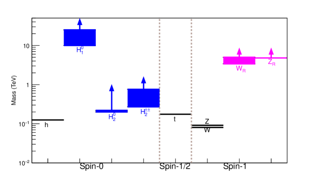
All the current LHC limits on the BSM particles in the LRSM are collected in Table 1 and also depicted in Fig. 1. Here are more details:
-
•
At the LHC, the boson in the LRSM can be produced via the right-handed charged quark currents. After its production, it can decay predominately into two quark jets (including the channel) and RHNs plus a charged lepton, i.e. (with ). If the RHNs are lighter than the boson, as a result of the Majorana nature of RHNs, the same-sign dilepton plus jets constitute a smoking-gun signal of the boson Keung:1983uu . Assuming , the current most stringent LHC data require that the mass TeV for a RHN mass TeV Aaboud:2018spl ; Aaboud:2019wfg . The dijet Aad:2019hjw ; Sirunyan:2019vgj and Sirunyan:2017ukk ; Sirunyan:2017vkm limits are relatively weaker, which are respectively 4 TeV and 3.4 TeV. The strongest limit of TeV is presented in Fig. 1.
-
•
The most stringent limits on the boson is from the dilepton data . The current dilepton limit on a sequential boson is 5.1 TeV Aad:2019fac . Following e.g. Ref. Chauhan:2018uuy , one can rescale the production cross section times branching fraction for the sequential model, which leads to the LHC dilepton limit of 4.82 TeV on the boson in the LRSM. This is shown in Fig. 1 as the limit. There are also dijet searches of the boson, however the corresponding limits are relatively weaker Aad:2019hjw ; Sirunyan:2019vgj .
-
•
At the leading order, the scalars , , and from the left-handed triplet have the same mass Zhang:2007da (see Table 5). The doubly-charged scalar can decay into either same-sign dilepton or same-sign bosons, i.e. , which constitute the most promising channels to probe at the LHC, and the branching fractions and depend on the Yukawa coupling and the left-handed triplet VEV . Assuming decays predominately into electrons and muons, the current LHC limits are around 770 to 870 GeV, depending on the flavor structure Aaboud:2017qph . In the di-tauon channel , the LHC limit is relatively weaker, i.e. 535 GeV CMS:2017pet .222 As the singly-charged scalar and doubly-charged scalar are mass degenerate at the leading order in the LRSM, here we have adopted the combined LHC limit from the pair production and the associate production . In these two channels, the separate channels are respectively 396 GeV and 479 GeV CMS:2017pet . If the doubly-charged scalar decays predominately into same-sign bosons, the LHC limits are much weaker, around 200 to 220 GeV Aaboud:2018qcu . There are also some searches of singly-charged scalar at the LHC Aaboud:2016dig ; Aaboud:2018gjj ; Sirunyan:2019hkq . However these searches assume is produced from its interaction with top and bottom quarks, therefore these limits are not applicable to in the LRSM which does not couple directly to the SM quarks. The strongest same-sign dilepton limits of GeV on (and also on other scalars from ) is shown in Fig. 1.
-
•
As the boson is very heavy, the TeV-scale right-handed doubly-charged scalar decays only into same-sign dileptons. The couplings of to the photon and boson have opposite signs, therefore the production cross section of at the LHC is smaller than that for the left-handed doubly-charged scalar . Rescaling the LHC13 cross section of by a factor of 1/2.4, The same-sign dilepton limits on turn out to be 271 to 760 GeV for all the six combinations of lepton flavors, which is presented in Fig. 1.
-
•
The scalars , and from the bidoublet are degenerate in mass at the leading order. and has tree-level flavor-changing neutral-current (FCNC) couplings to the SM quarks, and contribute to , and mixings significantly. As a result, their masses are required to be at least TeV, depending on the nature of left-right symmetry (either generalized parity or generalized charge conjugation), the hadronic uncertainties Ecker:1983uh ; Zhang:2007da ; Maiezza:2010ic ; Bertolini:2014sua and the potentially large QCD corrections Bernard:2015boz . The stringent FCNC limits on the heavy bidoublet scalars is shown in Fig. 1.
-
•
The neutral scalar from the right-handed triplet is hadrophobic, i.e. it does not couples directly to the SM quarks in the Lagrangian. It can be produced at the LHC and future higher energy colliders either in the scalar portal through coupling to the SM Higgs (and the heavy scalars and ), or in the gauge portal via coupling to the and bosons. Therefore the direct LHC limits are very weak Dev:2016vle ; Dev:2017dui . However, when it is sufficiently light, say at the GeV-scale, can be produced from (invisible) decay of the SM Higgs or even from the meson decays Dev:2016vle ; Dev:2017dui . More details can be found in Section 5.2.
-
•
The RHNs in the LRSM can be either very light, e.g. at the keV scale to be a warm DM Nemevsek:2012cd candidate, or very heavy at the scale, and there are almost no laboratory limits on their masses, although their mixings with the active neutrinos are tightly constrained in some regions of the parameter space Bolton:2019pcu . For simplicity, in the following sections we will set the masses of RHNs to be free parameters and neglect their mixings with the active neutrinos.
| Particle | Channel | Lower Limit | References |
|---|---|---|---|
| TeV | Aaboud:2019wfg ; Aaboud:2018spl | ||
| TeV | Aad:2019hjw ; Sirunyan:2019vgj | ||
| TeV | Sirunyan:2017ukk ; Sirunyan:2017vkm | ||
| TeV | Aad:2019fac | ||
| GeV | Aaboud:2017qph ; CMS:2017pet | ||
| (, , ) | GeV | Aaboud:2018qcu | |
| GeV | Aaboud:2017qph | ||
| , () | meson mixing | 10 - 25 TeV | Ecker:1983uh ; Zhang:2007da ; Maiezza:2010ic ; Bertolini:2014sua |
3 Phase transition in LRSM
3.1 One-loop effective potential
To study phase transitions in the LRSM, we consider the effective potential at finite temperature, which includes contributions of the one-loop corrections and daisy resummations. Renormalized in the scheme, the effective potential can be cast into the following form Basler:2018cwe
| (22) | |||||
where is the tree-level potential, is the Coleman-Weinberg one-loop effective potential Coleman:1973jx , and and are the thermal contributions at finite temperature. The term includes only the one-loop contributions, and denotes the high-order contributions from daisy diagrams. In Eq. (22) the sum runs over all the particles in the model. The scalar mass matrices in the LRSM can be found in Ref. Deshpande:1990ip , and the corresponding thermal self-energies are provided in Appendix A. As for the fermions, we consider only the third generation quarks and three RHNs. In the LRSM their masses are respectively
| (23) |
with the Yukawa couplings for top and bottom quarks in the SM, the RHN masses and the corresponding Yukawa coupling. In the following study, for the sake of simplicity, we will assume three RHNs are mass degenerate and does not have any mixings among them. The degrees of freedom and constants in Eq. (22) are given by
| (24) |
with for Weyl (Dirac) fermions, and the functions for bosons (fermions) are defined as
| (25) |
In the limit of small , we can use the approximations Basler:2018cwe :
| (26) | |||||
| (27) |
where
| (28) |
In this paper we focus on the phase transition at the scale, thus as an approximation all the effects of SM components on the symmetry breaking can be neglected. Neglecting the daisy contributions, the effective potential can be written down explicitly in the following form Cohen:1993nk :
| (29) |
where , , and can be expressed by the model parameters as
| (30) | |||||
| (31) | |||||
| (32) | |||||
| (33) | |||||
where is the mass for the particle , and is the renormalization scale. Since there are lots of scalars in the LRSM, we deliberately separate their contributions from the vector bosons and RHNs. The contributions of scalars for each of the terms in Eq. (30) to (33) can be written in terms of the scalar masses via
| (34) | |||||
| (35) | |||||
| (36) | |||||
| (37) | |||||
where we have defined . It should be pointed out that all the masses in Eqs. (34) to (37) depend upon the right-handed VEV instead of . It is observed that the RHNs can also contribute to the symmetry breaking via affecting the parameters , and , while the parameter receives only contributions from the scalars and gauge bosons.
As seen in Eqs. (33) and (37), the parameter receive not only tree-level contribution from the quartic coupling which corresponds to the mass via (see Table 5), but also loop-level contributions from the heavy scalars, gauge bosons and RHNs in the LRSM. In particular, when the quartic coupling is small, or equivalently the scalar is much smaller than the scale, which is the parameter space of interest for phase transition and GW production in the LRSM (cf. Figs. 2, 3 and 8), the loop-level contributions in Eq. (33) might dominate . Furthermore, depends also on the gauge coupling via the heavy gauge boson masses and .
To have strong FOPT, the cubic terms proportional to are crucial. In the limit of , the phase transition is of second-order. In the SM, the effective coefficient of term is dominated by the gauge boson contributions, while in the LRSM, it receives contributions from both the scalars and gauge bosons, As a result of the large degree of freedom in the scalar sector of LRSM, it is remarkable that the scalar contributions to can even be much larger. The order parameter describing the FOPT is given by , where is the non-vanishing location of the minimum at the critical temperature at which the effective potential has two degenerate minima. In the EW baryogenesis Kuzmin:1985mm ; Shaposhnikov:1986jp ; Shaposhnikov:1987tw , to avoid the washout effects in the broken phase within the bubble wall, a strong FOPT is typically required to satisfy the following condition
| (38) |
3.2 Strong first-order phase transition at the scale
The effective potential (22) is a function of temperature . Meanwhile, the minima of the effective potential vary when the temperature changes. In order to find the quantity which measures the strength of FOPT, we need to find both the critical temperature and the critical VEV .333There might be some theoretical uncertainties in perturbative calculations of FOPTs and resultant GWs, which can be found, e.g. in Ref. Croon:2020cgk . In term of the parametrization given in Eq. (29), the critical temperature can be approximately expressed as
| (39) |
Thus it is clear that . Therefore, it is justified to neglect the contributions of SM particles to the phase transition at the right-handed scale , since their masses are at most close to and their contributions are suppressed due to their tiny couplings to the right-handed triplet.
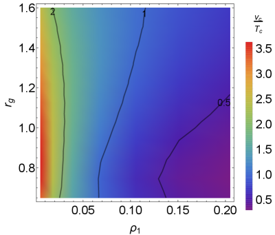
For given and heavy particle masses in the LRSM, the two key parameters and can be obtained from the effective potential (22) by requiring the two conditions and . In the numerical evaluations, we change the temperature from a sufficiently highly energy scale, say , toward lower values around the EW scale. A reasonable critical temperature for the phase transition is assumed to be within this range. The dependence of on the parameters in the LRSM is exemplified in Fig. 2, where in the numerical calculations we have included all the contributions in Eq. (22).
Taking into account all the theoretical and experimental constraints in Section 2, we first consider scenarios with the simplifications . In order to identify the parameter space where the phase transition is of first-order, we calculate at the critical temperature with different values of the quartic couplings , , , . When we calculate the dependence of on two of the quartic couplings, all others are fixed in the way that their corresponding scalar masses equal the mass, and the gauge coupling . To be concrete, we have set the renormalization scale to be the scale in Eq. (22). The corresponding results are shown in the first three panels of Fig. 2. The dependence of on the couplings and , and , and and are shown respectively in the upper left, upper right and lower left panels. The quantity is a dimensionless parameter and it is independent of the right-handed scale in the limit of . As the quartic couplings , , , are related directly to the scalar masses , , and (cf. Table 5), the dependence of on the quartic couplings in Fig. 2 can also be understood effectively as the dependence of on the mass ratios , , and . Through the gauge boson masses and , the parameter depends also on the gauge coupling ratio , or equivalently on the right-handed gauge coupling . This is shown in the lower right panel in Fig. 2; as seen in this figure, the limit on has a moderate or weak dependence on , depending on the value of .
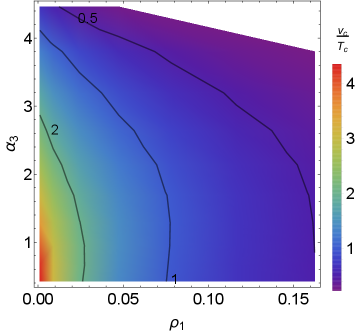
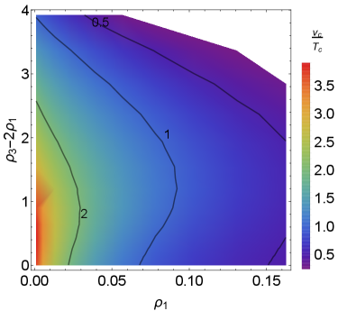
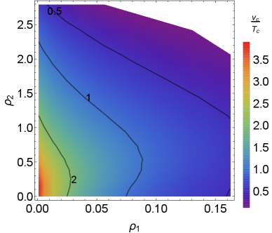
Given the information on in Fig. 2, a few more comments are now in order:
-
•
As seen in Fig. 2, a strong FOPT in the LRSM require a relatively small quartic coupling for the parameter space we are considering, which is qualitatively similar to the SM case where a light Higgs boson (say GeV) is needed in order to have a first-order EW phase transition Cline:2006ts . It turns out that a small (and resultantly light ) is not only crucial for the prospects of GWs in future experiments (cf. Fig. 8), but also triggers rich phenomenology for the searches of LLPs at the high-energy colliders and dedicated detectors Dev:2016vle ; Dev:2017dui .
-
•
The phase transition at the scale occurs when the neutral component of the right-handed triplet develops a non-vanishing VEV . As a result, the strong FOPT is more sensitive to the mass of , or equivalently to the value of , than other heavy scalar masses. This is also clearly demonstrated in the plots of Fig. 2. As seen in the upper left, upper right and lower left panels, the quartic coupling , and can reach up to order one, while in the Fig. 2.
-
•
Although the quartic couplings , and is less constrained by the FOPT than the critical coupling , as seen in the first three panels of Fig. 2, if either of these couplings is sufficiently large, it will invalidate the strong FOPT at the scale, no matter how small is. Meanwhile, the white areas in the plots of Fig. 2 indicate that in these regions the perturbation method starts to break down and theoretical predictions become more difficult.
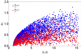
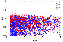
In Fig. 2 we have fixed some parameter in the LRSM and vary two of them. To see more details of the correlation of and the parameters in the LRSM, we take a more thorough scan of the parameter space of the LRSM. To be specific, we adopt the following ranges:
| (40) |
and apply all the theoretical and experimental constraints in Section 2. Here follows some comments:
-
•
We have chosen in order to satisfy the theoretical constraint in Eq. (21).
-
•
We have chosen in order to meet the requirement of the correct vacuum conditions given in Eq. (B).
-
•
It is known from Fig. 2 that the strongly FOPT need a small , therefore we have chosen .
-
•
has set to be larger than zero, as it corresponds to the masses of the left-handed triplet scalars (see Table 5).
-
•
The quartic coupling is not a free parameter here, as it is related to and the SM coupling via Eq. (52). As is always positive, it turn out that the quartic coupling .
-
•
We have chosen two benchmark values of TeV and TeV for the right-handed scale to examine the dependence of FOPT on . It turns out that the phase transition is almost independent of the values of , as expected.
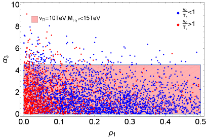
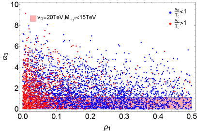
The resultant scatter plots of are presented in Fig. 3 as functions of the parameters and . The data points of strong FOPT with are shown in red while those with are in blue. When we set TeV and take the FCNC limit of TeV Zhang:2007da , the quartic coupling should meet the condition . The region shaded by the light pink in the left panel of Fig. 3 is excluded by such conditions. It is found that only a small amount of the data points can survive and have strong FOPT. When the scale is higher, say TeV, the quartic coupling is significantly smaller, i.e. . The region denoted by the light pink shaded region in the right panel of Fig. 3 is excluded. Then there will be more points that can have a strong FOPT with , as clearly shown in the right panel of Fig. 3.
4 Gravitational waves
The thermal stochastic GWs can be generated by three physics processes in phase transition Caprini:2015zlo : collisions of bubbles, sound waves (SWs) in the plasma after the bubble collision, and the MHD turbulence forming after the bubble collision. For non-runaway scenarios, GWs are dominated by the latter two sources Caprini:2015zlo , and the corresponding GW spectrum can be approximated as
| (41) |
The SW contribution has the form of Hindmarsh:2015qta
where is the frequency, and are respectively the number of relativistic degrees of freedom in the plasma and the Hubble parameter at the temperature , is the bubble wall velocity, describes the strength of phase transition, measures the rate of the phase transition, and
| (43) |
is the fraction of vacuum energy that is converted to bulk motion. The peak frequency is approximated by
| (44) |
The MHD turbulence contribution is Caprini:2009yp ; Binetruy:2012ze
where is the fraction of vacuum energy that is transformed into the MHD turbulence, is the inverse Hubble time at the GW production (red-shifted to today), and is given by
| (46) |
and the peak frequency is
| (47) |
As shown in the formula above, the gravitational wave spectrum from FOPTs are generally characterized by two parameters related to the phase transition, namely and Grojean:2006bp . The parameter is defined as the ratio of the vacuum energy density released at the phase transition temperature to the energy density of the universe in the radiation era, i.e.
| (48) |
where is the latent heat and can be expressed as
| (49) |
The denotes the difference of potential energy between the false vacuum and true vacuum, i.e. , which can be simply determined by and the parameters of LRSM.
The parameter describes the rate of variation of the bubble nucleation rate during phase transition, and its inverse describes the duration of phase transition. To describe rate of the phase transition, a dimensionless parameter is defined from the following equation
| (50) |
where denotes the three-dimensional Euclidean action of a critical bubble. The denotes the temperature when the phase transition is ended and can be determined by requiring that the probability for nucleating one bubble per horizon volume equals 1, i.e.
| (51) |
where is the probability of bubble nucleation per horizon volume, which can be expressed as , with Coleman:1977py ; Linde:1980tt ; Linde:1981zj . In this paper, is computed using the code CosmoTransitions Wainwright:2011kj to solve the bounce equation of bubbles.
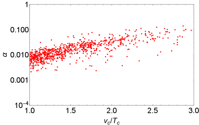
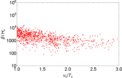
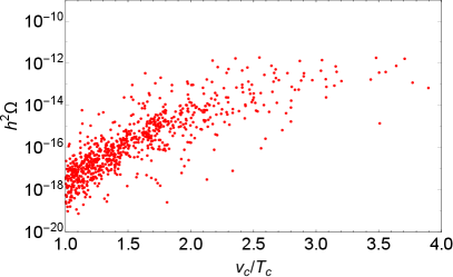
The parameters and set respectively the strength and time variation of GWs during the phase transition, and their typical values in the LRSM are shown respectively in the left and right panels of Fig. 4. As demonstrated by the data points, the value of varies roughly from to , and can range from to . In the numerical calculations, all the data points in Fig. 4 have strong FOPT.
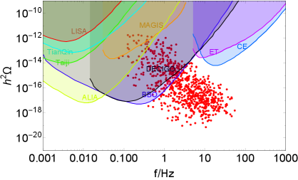
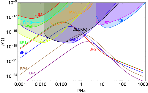
Assuming the bubble wall velocity , the corresponding GW signals of the data points in Fig. 4 are shown in Fig. 5. The correlation of the ratio and GW signal peaks are presented in the left panel. We can read from Fig. 4 and the left panel of Fig. 5 that with large the value is typically larger, thus yielding stronger GW signals. The GW strength and frequency peaks are shown in the right panel of Fig. 5. The potential sensitivities of LISA Audley:2017drz ; Cornish:2018dyw , TianQin Luo:2015ght , Taiji Guo:2018npi , ALIA Gong:2014mca , MAGIS Coleman:2018ozp , BBO Corbin:2005ny , DECIGO Musha:2017usi , ET Punturo:2010zz , and CE Evans:2016mbw are also depicted in the right panel of Fig. 5. As seen in this figure, the frequency peak in the LRSM can range from to Hz. Furthermore, there are some data points of the LRSM with frequencies in the range of roughly from to Hz and GW strength larger than , which can be detected in the future by BBO and DECIGO, or even by ALIA and MAGIS.
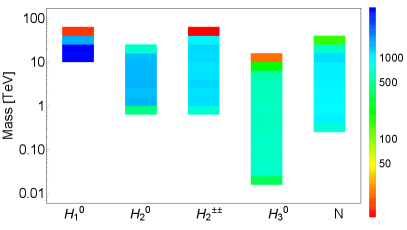
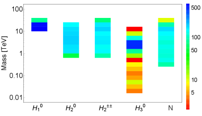
For the data points in Fig. 5 with strong FOPT, the mass spectra of the scalars , , , and the mass of RHNs are shown in the left panel of Fig. 6, and the mass spectra of these particles for the data points that are achievable in the BBO and DECIGO experiments are presented in the right panel of Fig. 6. The two plots of Fig. 6 clearly show that the masses of , and can reach up to few times 10 TeV, with their lower mass limits roughly round the experimental constraints in Section 2.3 (see also Table 1 and Fig. 1). The mass of can go to much smaller values, i.e. from 20 GeV up to 10 TeV. This can be easily understood: on one hand, the theoretical and experimental constraints on mass are rather weak (see Section 2); on the other hand, the strong FOPT and GW production in the LRSM favor a relatively light (see Figs. 2, 3 and 8). As seen in Fig. 6, the RHN masses can range roughly from 300 GeV up to 40 TeV. It is expected that the GW probe of and RHNs are largely complementary to the direct searches of them at the high-energy colliders, including the searches of long-lived and . See Section 5.2 for more details.
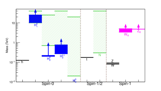
For the purpose of comparison, we present in Fig. 7 the experimental limits on the masses of , and in Fig. 1 and the GW sensitive ranges of the masses of , , , and in Fig. 6, where the mass ranges within the sensitivities of GW detectors are represented by green hatched areas. It is clear that the GWs from phase transition can probe a large region of parameter space in the LRSM that goes beyond the current collider limits.
To expose more features of GWs from the phase transition at the scale in the LRSM, we have chosen five specific BPs. For the sake of concreteness and simplification, we have chosen TeV, , and set the quartic couplings , . The BSM particle masses , , , and are collected in the first few columns of Table 2. The resultant , , and the parameters and are also shown in Table 2. The GW spectra as function of the frequency for the five BPs are presented in Fig. 8. There are a few comments on the five BPs.
| BPs | BP1 | BP2 | BP3 | BP4 | BP5 |
|---|---|---|---|---|---|
| 10 TeV | 10 TeV | 10 TeV | 10 TeV | 10 TeV | |
| 8 TeV | 8 TeV | 8 TeV | 8 TeV | 10 TeV | |
| 40 GeV | 500 GeV | 1 TeV | 2 TeV | 2 TeV | |
| 8 TeV | 8 TeV | 8 TeV | 8 TeV | 10 TeV | |
| 1 TeV | 1 TeV | 1 TeV | 1 TeV | 2 TeV | |
| 8.02 TeV | 8.01 TeV | 7.98 TeV | 7.72 TeV | 7.18 TeV | |
| 3.42 TeV | 3.50 TeV | 3.73 TeV | 4.49 TeV | 5.44 TeV | |
| 2.17 TeV | 2.27 TeV | 2.75 TeV | 3.92 TeV | 4.89 TeV | |
| 0.056 | 0.053 | 0.037 | 0.019 | 0.0083 | |
| 0.18 | 0.16 | 0.11 | 0.053 | 0.037 | |
| 265 | 272 | 493 | 1373 | 1908 | |
| 0.16 | 0.16 | 0.13 | 0.10 | 0.15 |
-
•
It is clear in Fig. 8 that the BPs (from BP1 to BP4) with the same values of , , and but different can be probed in the future by BBO and DECIGO, and even by ALIA and MAGIS. It seems that the mass , or equivalently the quartic coupling , is crucial for the GWs in the LRSM. The BPs (like BP5) with a heavier , or equivalently larger , tends to generate a small and large , and thus produce weaker GW signals with a larger frequency. This is consistent with the findings in Ref. Brdar:2019fur . The BPs BP1 and BP2 with mass below TeV-scale can produce GWs of order with frequency at around 0.1 Hz, far above the prospects of BBO and DECIGO. The BP4 with a 2 TeV can only produce GWs of order with frequency peaked at 1 Hz, which can be marginally detected by BBO and DECIGO.
-
•
Comparing BP4 and BP5, it is clear that only the masses of , and are heavier in BP5 than in BP4, while all other parameters are the same. As seen in Fig. 8, the GW signal in BP5 is so weak that it can escape the detection of all the planned GW experiments in the figure. This reveals that the masses , and , or equivalently the couplings , and , are also important for GW production in the LRSM. More data points in the numerical calculations reveal that the coupling is also very important for the GW signals in the LRSM.
5 Complementarity of GW signal and collider searches of LRSM
In spite of the large number of BSM scalars, fermions and gauge bosons in the LRSM and the larger number of quartic couplings in the potential (8), it is phenomenologically meaningful to examine the role of some couplings, or equivalently the BSM particle masses, in the strong FOPT and the subsequent GW production in the early universe, as well as the potential correlations of GWs to the direct laboratory searches of these particles and the SM precision data at the high-energy colliders. In this section, we will elaborate on (i) the effects of the quartic coupling in the scalar potential (8) which corresponds to the self-coupling in the SM, and (ii) the complementarity of GW signal, the collider searches of (light) and the heavy (or light) RHNs in the LRSM.
5.1 Self-couplings of SM-like Higgs boson in the LRSM
| models | mass squared | ||
|---|---|---|---|
| SM | |||
| LRSM |
It is interesting to examine how the self-coupling of the SM-like Higgs boson can be affected by the BSM scalars in the LRSM. The SM-like Higgs mass square, the trilinear coupling and the quartic coupling in the SM and LRSM are collected in Table 3. Comparing the mass square of in the SM and LRSM, we can approximately identify the following relation among the SM and LRSM quartic couplings Dev:2016dja ; Maiezza:2016ybz
| (52) |
As seen in the third column of Fig. 3, the trilinear coupling of the SM-like Higgs in the LRSM only differs from the SM value by a small amount of Dev:2016dja ; Maiezza:2016ybz . On the contrary, the quartic coupling in the LRSM might be significantly different from the SM prediction: as shown in the last column of Table 3 Dev:2016dja ; Maiezza:2016ybz ,
| (53) |
In other words, at the leading-order of the approximations of , the difference of quartic coupling of SM-like Higgs boson in the SM and LRSM is dominated by the term. As the FOPT and GW in the LRSM favor a small coupling, the difference in Eq. (53) tends to be significant for sufficiently large .
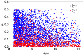
Adopting the parameter ranges in Eq. (40) and taking into account the theoretical and experimental limits in Section 2, the scatter plots of the quartic coupling and the couplings , and are shown respectively in the left, middle and right panels of Fig. 9, where the data points with strong FOPT is shown in red, while those with are in blue. It is very clear in Fig. 9 that the deviation of the quartic scalar coupling from the SM value is always positive and can be very large, even up to the order of 10, as expected in Table 3 and Eq. (53). We can also read from the left and middle panels of Fig. 9 that a large deviation of the quartic coupling of SM-like Higgs need a relatively small and/or large . As given in Eq. (33), a large tends to decrease , thus increasing the value of . However, if is too large, say , a negative will be obtained which leads to a non-stable vacuum. Thus, the phase transition and GW in the LRSM favor a Yukawa coupling to .
On the experimental side, the combined results of di-Higgs searches can be found e.g. in Refs. Sirunyan:2018ayu ; Aad:2019uzh . Data from LHC 13 TeV with a luminosity of fb-1 only set a weak constraint . The LHC 14 TeV with an integrated luminosity of 3 ab-1 can probe the trilinear coupling of SM Higgs within the range of Barger:2013jfa , while the future 100 TeV collider with a luminosity of 30 ab-1 can help to improve the sensitivity up to Kilian:2017nio . However, this is not precise enough to see the deviation of trilinear coupling in the LRSM, which is of order or smaller.
Although the quartic coupling measurements can not be greatly improved at hadronic colliders Kilian:2017nio ; Chen:2015gva , a future muon collider with the center-of-mass energy of 14 TeV and a luminosity of 33 ab-1 can probe a deviation of the quartic Higgs self-coupling at the level of Chiesa:2020awd . This can probe a sizable region of parameter space in Fig. 9.
5.2 Searches of and RHNs in the LRSM
As implied by the BPs in Figs. 6 and 8, the GW signals favor a relatively light in the LRSM, and this can be correlated to the direct searches of a (light) at the high-energy frontier. At the high-energy colliders, the scalar can be produced in two portals Dev:2016dja :
-
•
The scalar portal, i.e. the production of through its coupling to the SM Higgs . This includes the channels and . The production amplitudes in both the two channels are proportional to the quartic coupling . As the trilinear couplings and are respectively proportional to the VEVs and , even if is small say , the production cross sections are still sizable. Assuming and TeV, the prospects of at the LHC 14 TeV with an integrated luminosity of 3 ab-1 and the future 100 TeV collider with a luminosity of 30 ab-1 are shown as the yellow and brown bands in Fig. 10 Dev:2016dja .
-
•
The gauge portal, i.e. the production of through its couplings to the heavy and gauge bosons, in the Higgsstrahlung process (with ) and the vector boson fusion (VBF) process . In light of the current direct LHC constraints on and (see Section 2.3), the prospects of at the LHC in these channels are very limited, which however can be largely improved at future 100 TeV colliders. The FCC-hh prospects in the and channels are shown respectively as the green and magenta bands in Fig. 10.
In obtaining both the scalar and gauge portal prospects, we have set a lower bound on the mass, i.e. GeV, such that the exotic decay of the SM Higgs is kinematically forbidden Curtin:2013fra .
The scalar mixes with the SM Higgs and the heavy bidoublet scalar , which induces the tree-level FCNC couplings of to the SM quarks. Therefore for sufficiently light , it can be produced from flavor-changing meson decays, such as Dev:2016vle ; Dev:2017dui . The high-precision SM meson data have set very severe constraints on the mixing angles of with and . Therefore in a large region of parameter space the light decays predominately into two photons through the and heavy charged scalar loops in the LRSM. Suppressed by the heavy particle masses in the loops, the scalar tends to be long-lived, and can thus be searched in the multi-purpose detectors at the high-energy colliders as well as the dedicated LLP experiments therein. The prospects of long-lived at the LHC 14 TeV, FCC-hh, and MATHUSLA Curtin:2018mvb are presented Fig. 10 respectively as the orange, red and pink bands Dev:2016vle ; Dev:2017dui .
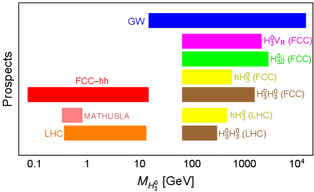
The GW prospect of in Fig. 6 is indicated by the blue band in Fig. 10. As clearly seen in Fig. 10, the direct searches of at the LHC and future 100 TeV colliders can probe a mass range of roughly 100 GeV up to 3 TeV, while the searches of a long-lived at the high-energy colliders can cover the mass range of 10 GeV down to 100 MeV. As a new avenue to probe the phase transition in the LRSM, GWs are sensitive to a wide mass range of , from the 10 GeV scale up to 10 TeV, which is largely complementary to the searches of (light) at the high-energy colliders.
Note that one of the important decay modes of is the RHN channel, i.e. , which will induce the strikingly clean signal of same-sign dilepton plus jets Dev:2016dja ; Maiezza:2015lza ; Nemevsek:2016enw . The heavy RHNs can also be produced through their gauge couplings to the and bosons, e.g. the smoking-gun Keung-Senjanović signal at the high-energy colliders Keung:1983uu . If the RHNs are very light, say below 100 GeV scale, the decay widths of RHNs will be highly suppressed by mass, which makes the RHNs long-lived Helo:2013esa ; Cottin:2018kmq . The light long-lived RHNs can be searched directly at the high-energy colliders via displaced vertex, or even from meson decays Helo:2010cw ; Cvetic:2010rw ; Drewes:2015iva ; Bondarenko:2018ptm . The prospects of RHNs at the high-energy colliders and in meson decays depend largely on the heavy scalar or gauge boson masses (see also Mitra:2016kov ; Ruiz:2017nip ). However, it is worth pointing out that, as seen in Fig. 6, GWs are sensitive to the RHN masses in the range of 200 GeV up to 40 TeV, which is largely complementary to the direct searches of (light) RHNs at the high-energy frontier.
6 Discussions and Conclusion
Before the conclusion we would like to comment on some open questions in the phase transition and GW production in the LRSM:
-
•
In the calculations we have assumed that at the epoch of phase transition the bubbles expanding in the plasma can reach a relativistic terminal velocity, i.e. the non-runaway scenarios, where the velocity of bubble wall is taken to be in our analysis, which corresponds to the denotation case Espinosa:2010hh . A recent numerical analysis Cutting:2019zws has revealed that the SW contribution might be suppressed by a factor of in the deflagration case when where the reheated droplet can suppress the formation of GW signals. While there is no such a huge suppression for the denotation case with , our results could still be valid, although the GW signals might be suppressed by a factor two or three. The bubble wave velocity, in principle, can be computed from the parameters of a given model, as demonstrated in Moore:1995ua ; Moore:1995si ; Bodeker:2009qy . Furthermore, according to the recent calculations in Ref. Guo:2020grp , it is found that the finite lifetime of SWs can lead to a suppression factor , which can be parameterized in the following form Fornal:2020esl
(54) We have calculated the factors for the five BPs in Table 2, and listed it in the last row of this table. It is observed that the GW signals in these BPs might be suppressed by up to a factor of 6 to 10. It might be interesting to explore how the model parameters of LRSM can affect the bubble wall velocity and the effects of the suppression factor , which will be a topic for our future study.
-
•
It is remarkable that for the scalar , which is mainly the CP-even neutral component of the right-handed triplet , both the theoretical and experimental constraints on it are very weak. As a result, its mass could span a wide range, say from below GeV-scale up to tens of TeV. In the case that all other new particles in the LRSM are heavier than 5 TeV but with a relatively light below the TeV-scale (for instance the BPs BP1 and BP2 in Table 2), at the scale below 1 TeV, the scalar potential of LRSM given in Eq. (8) can be reduced to the effective model with the SM extended by a real singlet , where the scalar potential has the following form:
(55) The trilinear and quartic couplings in Eq. (55) can be written as functions of the right-handed VEV and the quartic couplings in the LRSM, which are collected in Table 4. Obviously, when is switched off, will not affect the EW phase transition directly, and the EW phase transition should be of second-order as in the SM. When is switched on, it might be interesting to examine whether the light can affect the phase transitions at both the scale and the EW scale. When it is possible, a multi-step strong FOPT could be expected Angelescu:2018dkk .
| trilinear couplings | expressions |
| quartic couplings | expressions |
To summarize, in this paper we have studied the prospects of GW signals from phase transition in the minimal LRSM with a bidoublet , a left-handed triplet and a right-handed triplet , which is a well-motivated framework to restore parity and accommodate the seesaw mechanisms for tiny neutrino masses at the TeV-scale. We have considered the theoretical limits on the LRSM from perturbativity, unitarity, vacuum stability and correct vacuum criteria, as well as the experimental constraints on the heavy gauge bosons and the BSM scalars. The experimental limits are collected in Table 1 and Fig. 1.
With these theoretical and experimental constraints taken into account, we have analyzed the parameter space of strong FOPT and the resultant GWs in the LRSM. As demonstrated in Figs. 2, 3 and 9, the strong FOPT at the scale favors relatively small quartic and Yukawa couplings, which corresponds to relatively light BSM scalars and RHNs. The GWs for some BPs in the LRSM in Fig. 5 reveal that the phase transition in the LRSM can generate the GW signals of to , with a frequency ranging from 0.1 to 10 Hz, which can be probed by the experiments BBO and DECIGO, or even by ALIA and MAGIS. Setting TeV, as seen in Fig. 6, the GWs are sensitive to the following mass ranges:
-
•
The heavy bidoublet scalars , , , the scalars , , and from the left-handed triplet , and the doubly-charged scalar from the right-handed triplet , with masses up to tens of TeV, with the lower bounds of their masses roughly set by the experimental limits in Fig. 1.
-
•
The scalar with mass in the range of roughly from 20 GeV up to 10 TeV. As presented in Fig. 10, the GW prospects of are largely complementary to the direct searches of heavy at the LHC and future 100 TeV colliders, and the searches of light from displaced vertex signals at the LHC, future higher energy colliders, and the LLP experiments such as MATHUSLA.
-
•
The RHNs with masses from roughly 300 GeV up to 40 TeV. The GW sensitivity of is also largely complementary to the direct searches of prompt signals and displaced vertices from RHNs at the high-energy colliders, as well as the production of RHNs from meson decays.
The GW spectra in Fig. 8 for the BPs in Table 2 shows that the quartic coupling is crucially important for both the frequency and strength of the GW signals in the LRSM, while other couplings such as , , and are also important. In addition, the precision measurement of the quartic coupling of the SM Higgs at a future muon collider can probe a sizable region of the parameter space in LRSM, which can have strong FOPT and observable GW signals, as exemplified in Fig. 9.
Acknowledgments
This work is supported by the Natural Science Foundation of China under the grant no. 11575005. Y.Z. would like to thank P. S. Bhupal Dev and Yiyang Zhang for the helpful discussions at the early stage of this paper. The authors would also like to thank Dr. Yi-Dian Chen, Dr. Huaike Guo, Dr. Bartosz Fornal, Dr. White Graham Albert, and Dr. Zhi-Wei Wang for some useful information.
Appendix A Mass matrices and thermal self-energies
| physical states | mass squared |
|---|---|
In the LRSM with a bidoublet , a left-handed triplet and a right-handed triplet , there are 20 degrees of freedom in the scalar sector. In this paper, for simplicity we assume there is no CP violation in the scalar sector, i.e. the CP phase in the potential (8) and the phases in the VEVs (9). In the limit of , all the physical scalars and their masses are collected in Table 5. The corresponding mass matrix elements can be found e.g. in Ref. Deshpande:1990ip . In the basis of , the thermal self-energy of the real neutral components are respectively:
| (57) | |||||
| (58) | |||||
| (59) | |||||
| (60) |
All the rest elements are related to the ones above via . The thermal self-energy for the imaginary components of the neutral scalars is very similar to that for the real components. In the basis of , the elements are respectively:
| (61) |
For the singly charged fields, in the basis of , the thermal self-energy is the same as that for the real neutral components, i.e. . For the doubly-charged scalars, in the basis of , the corresponding self-energy is given by
| (62) |
For the neutral gauge bosons, in the basis of , the self-energy matrix reads
| (63) |
while for the singly-charged gauge bosons, in the basis of , the self-energy matrix is
| (64) |
Appendix B Conditions for vacuum stability and correct vacuum
The sufficient but not necessary conditions for vacuum stability and correct vacuum in the LRSM are worked out in Chauhan:2019fji and listed below (simple analytic formula can only be obtained in the condition ):
| (65) |
where , with the definition , the parameter is defined via , and
| (70) |
where the condition structure “” means needs to be checked if and only if the condition is true. In this paper, we have chosen , which corresponds to the case of .
References
- (1) ATLAS collaboration, Observation of a new particle in the search for the Standard Model Higgs boson with the ATLAS detector at the LHC, Phys. Lett. B716 (2012) 1 [1207.7214].
- (2) CMS collaboration, Observation of a new boson at a mass of 125 GeV with the CMS experiment at the LHC, Phys. Lett. B716 (2012) 30 [1207.7235].
- (3) D. E. Morrissey, T. Plehn and T. M. P. Tait, Physics searches at the LHC, Phys. Rept. 515 (2012) 1 [0912.3259].
- (4) R. N. Mohapatra and A. Y. Smirnov, Neutrino Mass and New Physics, Ann. Rev. Nucl. Part. Sci. 56 (2006) 569 [hep-ph/0603118].
- (5) V. Sahni, Dark matter and dark energy, Lect. Notes Phys. 653 (2004) 141 [astro-ph/0403324].
- (6) A. G. Cohen, D. B. Kaplan and A. E. Nelson, Progress in electroweak baryogenesis, Ann. Rev. Nucl. Part. Sci. 43 (1993) 27 [hep-ph/9302210].
- (7) V. A. Rubakov and M. E. Shaposhnikov, Electroweak baryon number nonconservation in the early universe and in high-energy collisions, Usp. Fiz. Nauk 166 (1996) 493 [hep-ph/9603208].
- (8) M. Trodden, Electroweak baryogenesis, Rev. Mod. Phys. 71 (1999) 1463 [hep-ph/9803479].
- (9) D. E. Morrissey and M. J. Ramsey-Musolf, Electroweak baryogenesis, New J. Phys. 14 (2012) 125003 [1206.2942].
- (10) The International Linear Collider Technical Design Report - Volume 2: Physics, 1306.6352.
- (11) M. Ahmad et al., CEPC-SPPC Preliminary Conceptual Design Report. 1. Physics and Detector, .
- (12) https://fcc.web.cern.ch/Pages/default.aspx.
- (13) J. Tang et al., Concept for a Future Super Proton-Proton Collider, 1507.03224.
- (14) A. Sakharov, Violation of CP Invariance, C asymmetry, and baryon asymmetry of the universe, Sov. Phys. Usp. 34 (1991) 392.
- (15) R.-G. Cai, Z. Cao, Z.-K. Guo, S.-J. Wang and T. Yang, The Gravitational-Wave Physics, Natl. Sci. Rev. 4 (2017) 687 [1703.00187].
- (16) A. Kosowsky, M. S. Turner and R. Watkins, Gravitational radiation from colliding vacuum bubbles, Phys. Rev. D 45 (1992) 4514.
- (17) A. Kosowsky and M. S. Turner, Gravitational radiation from colliding vacuum bubbles: envelope approximation to many bubble collisions, Phys. Rev. D 47 (1993) 4372 [astro-ph/9211004].
- (18) S. J. Huber and T. Konstandin, Gravitational Wave Production by Collisions: More Bubbles, JCAP 0809 (2008) 022 [0806.1828].
- (19) A. Kosowsky, M. S. Turner and R. Watkins, Gravitational waves from first order cosmological phase transitions, Phys. Rev. Lett. 69 (1992) 2026.
- (20) M. Kamionkowski, A. Kosowsky and M. S. Turner, Gravitational radiation from first order phase transitions, Phys. Rev. D 49 (1994) 2837 [astro-ph/9310044].
- (21) C. Caprini, R. Durrer and G. Servant, Gravitational wave generation from bubble collisions in first-order phase transitions: An analytic approach, Phys. Rev. D 77 (2008) 124015 [0711.2593].
- (22) M. Hindmarsh, S. J. Huber, K. Rummukainen and D. J. Weir, Gravitational waves from the sound of a first order phase transition, Phys. Rev. Lett. 112 (2014) 041301 [1304.2433].
- (23) J. Giblin, John T. and J. B. Mertens, Vacuum Bubbles in the Presence of a Relativistic Fluid, JHEP 12 (2013) 042 [1310.2948].
- (24) J. T. Giblin and J. B. Mertens, Gravitional radiation from first-order phase transitions in the presence of a fluid, Phys. Rev. D 90 (2014) 023532 [1405.4005].
- (25) M. Hindmarsh, S. J. Huber, K. Rummukainen and D. J. Weir, Numerical simulations of acoustically generated gravitational waves at a first order phase transition, Phys. Rev. D92 (2015) 123009 [1504.03291].
- (26) C. Caprini and R. Durrer, Gravitational waves from stochastic relativistic sources: Primordial turbulence and magnetic fields, Phys. Rev. D 74 (2006) 063521 [astro-ph/0603476].
- (27) T. Kahniashvili, A. Kosowsky, G. Gogoberidze and Y. Maravin, Detectability of Gravitational Waves from Phase Transitions, Phys. Rev. D 78 (2008) 043003 [0806.0293].
- (28) T. Kahniashvili, L. Campanelli, G. Gogoberidze, Y. Maravin and B. Ratra, Gravitational Radiation from Primordial Helical Inverse Cascade MHD Turbulence, Phys. Rev. D 78 (2008) 123006 [0809.1899].
- (29) T. Kahniashvili, L. Kisslinger and T. Stevens, Gravitational Radiation Generated by Magnetic Fields in Cosmological Phase Transitions, Phys. Rev. D 81 (2010) 023004 [0905.0643].
- (30) C. Caprini, R. Durrer and G. Servant, The stochastic gravitational wave background from turbulence and magnetic fields generated by a first-order phase transition, JCAP 0912 (2009) 024 [0909.0622].
- (31) C. Grojean and G. Servant, Gravitational Waves from Phase Transitions at the Electroweak Scale and Beyond, Phys. Rev. D75 (2007) 043507 [hep-ph/0607107].
- (32) J. Ellis, M. Lewicki, J. M. No and V. Vaskonen, Gravitational wave energy budget in strongly supercooled phase transitions, JCAP 1906 (2019) 024 [1903.09642].
- (33) TianQin collaboration, TianQin: a space-borne gravitational wave detector, Class. Quant. Grav. 33 (2016) 035010 [1512.02076].
- (34) W.-H. Ruan, Z.-K. Guo, R.-G. Cai and Y.-Z. Zhang, Taiji Program: Gravitational-Wave Sources, Int. J. Mod. Phys. A 35 (2020) 2050075 [1807.09495].
- (35) LISA collaboration, Laser Interferometer Space Antenna, 1702.00786.
- (36) T. Robson, N. J. Cornish and C. Liu, The construction and use of LISA sensitivity curves, Class. Quant. Grav. 36 (2019) 105011 [1803.01944].
- (37) X. Gong et al., Descope of the ALIA mission, J. Phys. Conf. Ser. 610 (2015) 012011 [1410.7296].
- (38) MAGIS-100 collaboration, Matter-wave Atomic Gradiometer InterferometricSensor (MAGIS-100) at Fermilab, PoS ICHEP2018 (2019) 021 [1812.00482].
- (39) DECIGO Working group collaboration, Space gravitational wave detector DECIGO/pre-DECIGO, Proc. SPIE Int. Soc. Opt. Eng. 10562 (2017) 105623T.
- (40) V. Corbin and N. J. Cornish, Detecting the cosmic gravitational wave background with the big bang observer, Class. Quant. Grav. 23 (2006) 2435 [gr-qc/0512039].
- (41) LIGO Scientific collaboration, Exploring the Sensitivity of Next Generation Gravitational Wave Detectors, Class. Quant. Grav. 34 (2017) 044001 [1607.08697].
- (42) M. Punturo et al., The Einstein Telescope: A third-generation gravitational wave observatory, Class. Quant. Grav. 27 (2010) 194002.
- (43) LIGO Scientific collaboration, Gravitational wave astronomy with LIGO and similar detectors in the next decade, 1904.03187.
- (44) The LIGO Scientific Collaboration, LIGO DCC-T1400316 (2014).
- (45) LIGO Scientific, Virgo collaboration, Observation of Gravitational Waves from a Binary Black Hole Merger, Phys. Rev. Lett. 116 (2016) 061102 [1602.03837].
- (46) LIGO Scientific, Virgo collaboration, GW170817: Observation of Gravitational Waves from a Binary Neutron Star Inspiral, Phys. Rev. Lett. 119 (2017) 161101 [1710.05832].
- (47) P. Mészáros, D. B. Fox, C. Hanna and K. Murase, Multi-Messenger Astrophysics, Nature Rev. Phys. 1 (2019) 585 [1906.10212].
- (48) P. S. B. Dev and A. Mazumdar, Probing the Scale of New Physics by Advanced LIGO/VIRGO, Phys. Rev. D93 (2016) 104001 [1602.04203].
- (49) D. J. Weir, Gravitational waves from a first order electroweak phase transition: a brief review, Phil. Trans. Roy. Soc. Lond. A376 (2018) 20170126 [1705.01783].
- (50) F. P. Huang, Y. Wan, D.-G. Wang, Y.-F. Cai and X. Zhang, Hearing the echoes of electroweak baryogenesis with gravitational wave detectors, Phys. Rev. D94 (2016) 041702 [1601.01640].
- (51) P. Huang, A. J. Long and L.-T. Wang, Probing the Electroweak Phase Transition with Higgs Factories and Gravitational Waves, Phys. Rev. D94 (2016) 075008 [1608.06619].
- (52) I. P. Ivanov, Building and testing models with extended Higgs sectors, Prog. Part. Nucl. Phys. 95 (2017) 160 [1702.03776].
- (53) V. Vaskonen, Electroweak baryogenesis and gravitational waves from a real scalar singlet, Phys. Rev. D95 (2017) 123515 [1611.02073].
- (54) A. Beniwal, M. Lewicki, J. D. Wells, M. White and A. G. Williams, Gravitational wave, collider and dark matter signals from a scalar singlet electroweak baryogenesis, JHEP 08 (2017) 108 [1702.06124].
- (55) A. Alves, T. Ghosh, H.-K. Guo, K. Sinha and D. Vagie, Collider and Gravitational Wave Complementarity in Exploring the Singlet Extension of the Standard Model, JHEP 04 (2019) 052 [1812.09333].
- (56) N. Chen, T. Li, Y. Wu and L. Bian, Complementarity of the future colliders and gravitational waves in the probe of complex singlet extension to the standard model, Phys. Rev. D101 (2020) 075047 [1911.05579].
- (57) M. Kakizaki, S. Kanemura and T. Matsui, Gravitational waves as a probe of extended scalar sectors with the first order electroweak phase transition, Phys. Rev. D92 (2015) 115007 [1509.08394].
- (58) K. Hashino, M. Kakizaki, S. Kanemura and T. Matsui, Synergy between measurements of gravitational waves and the triple-Higgs coupling in probing the first-order electroweak phase transition, Phys. Rev. D94 (2016) 015005 [1604.02069].
- (59) K. Hashino, M. Kakizaki, S. Kanemura, P. Ko and T. Matsui, Gravitational waves and Higgs boson couplings for exploring first order phase transition in the model with a singlet scalar field, Phys. Lett. B766 (2017) 49 [1609.00297].
- (60) Z. Kang, P. Ko and T. Matsui, Strong first order EWPT & strong gravitational waves in Z3-symmetric singlet scalar extension, JHEP 02 (2018) 115 [1706.09721].
- (61) J. M. Cline and P.-A. Lemieux, Electroweak phase transition in two Higgs doublet models, Phys. Rev. D55 (1997) 3873 [hep-ph/9609240].
- (62) P. Basler, M. Krause, M. Muhlleitner, J. Wittbrodt and A. Wlotzka, Strong First Order Electroweak Phase Transition in the CP-Conserving 2HDM Revisited, JHEP 02 (2017) 121 [1612.04086].
- (63) G. C. Dorsch, S. J. Huber, T. Konstandin and J. M. No, A Second Higgs Doublet in the Early Universe: Baryogenesis and Gravitational Waves, JCAP 1705 (2017) 052 [1611.05874].
- (64) F. P. Huang and J.-H. Yu, Exploring inert dark matter blind spots with gravitational wave signatures, Phys. Rev. D98 (2018) 095022 [1704.04201].
- (65) X. Wang, F. P. Huang and X. Zhang, Gravitational wave and collider signals in complex two-Higgs doublet model with dynamical CP-violation at finite temperature, Phys. Rev. D 101 (2020) 015015 [1909.02978].
- (66) A. Paul, U. Mukhopadhyay and D. Majumdar, Gravitational Wave Signatures from Domain Wall and Strong First-Order Phase Transitions in a Two Complex Scalar extension of the Standard Model, 2010.03439.
- (67) M. Chala, M. Ramos and M. Spannowsky, Gravitational wave and collider probes of a triplet Higgs sector with a low cutoff, Eur. Phys. J. C 79 (2019) 156 [1812.01901].
- (68) R. Apreda, M. Maggiore, A. Nicolis and A. Riotto, Gravitational waves from electroweak phase transitions, Nucl. Phys. B631 (2002) 342 [gr-qc/0107033].
- (69) S. J. Huber, T. Konstandin, G. Nardini and I. Rues, Detectable Gravitational Waves from Very Strong Phase Transitions in the General NMSSM, JCAP 03 (2016) 036 [1512.06357].
- (70) S. J. Huber and T. Konstandin, Production of gravitational waves in the nMSSM, JCAP 05 (2008) 017 [0709.2091].
- (71) S. Demidov, D. Gorbunov and D. Kirpichnikov, Gravitational waves from phase transition in split NMSSM, Phys. Lett. B 779 (2018) 191 [1712.00087].
- (72) M. Chala, G. Nardini and I. Sobolev, Unified explanation for dark matter and electroweak baryogenesis with direct detection and gravitational wave signatures, Phys. Rev. D94 (2016) 055006 [1605.08663].
- (73) S. Bruggisser, B. Von Harling, O. Matsedonskyi and G. Servant, Electroweak Phase Transition and Baryogenesis in Composite Higgs Models, JHEP 12 (2018) 099 [1804.07314].
- (74) L. Bian, Y. Wu and K.-P. Xie, Electroweak phase transition with composite Higgs models: calculability, gravitational waves and collider searches, JHEP 12 (2019) 028 [1909.02014].
- (75) M. Jarvinen, C. Kouvaris and F. Sannino, Gravitational Techniwaves, Phys. Rev. D81 (2010) 064027 [0911.4096].
- (76) Y. Chen, M. Huang and Q.-S. Yan, Gravitation waves from QCD and electroweak phase transitions, JHEP 05 (2018) 178 [1712.03470].
- (77) K. Miura, H. Ohki, S. Otani and K. Yamawaki, Gravitational Waves from Walking Technicolor, JHEP 10 (2019) 194 [1811.05670].
- (78) K. Fujikura, K. Kamada, Y. Nakai and M. Yamaguchi, Phase Transitions in Twin Higgs Models, JHEP 12 (2018) 018 [1810.00574].
- (79) D. Croon, T. E. Gonzalo and G. White, Gravitational Waves from a Pati-Salam Phase Transition, JHEP 02 (2019) 083 [1812.02747].
- (80) W.-C. Huang, F. Sannino and Z.-W. Wang, Gravitational Waves from Pati-Salam Dynamics, Phys. Rev. D102 (2020) 095025 [2004.02332].
- (81) B. Fornal, S. A. Gadam and B. Grinstein, Left-Right SU(4) Vector Leptoquark Model for Flavor Anomalies, Phys. Rev. D99 (2019) 055025 [1812.01603].
- (82) B. Fornal, Gravitational Wave Signatures of Lepton Universality Violation, 2006.08802.
- (83) R. Zhou, W. Cheng, X. Deng, L. Bian and Y. Wu, Electroweak phase transition and Higgs phenomenology in the Georgi-Machacek model, JHEP 01 (2019) 216 [1812.06217].
- (84) P. S. B. Dev, F. Ferrer, Y. Zhang and Y. Zhang, Gravitational Waves from First-Order Phase Transition in a Simple Axion-Like Particle Model, JCAP 1911 (2019) 006 [1905.00891].
- (85) L. Delle Rose, G. Panico, M. Redi and A. Tesi, Gravitational Waves from Supercool Axions, JHEP 04 (2020) 025 [1912.06139].
- (86) A. Ghoshal and A. Salvio, Gravitational waves from fundamental axion dynamics, JHEP 12 (2020) 049 [2007.00005].
- (87) H. Yu, Z.-C. Lin and Y.-X. Liu, Gravitational waves and extra dimensions: a short review, Commun. Theor. Phys. 71 (2019) 991 [1905.10614].
- (88) A. Ahriche, K. Hashino, S. Kanemura and S. Nasri, Gravitational Waves from Phase Transitions in Models with Charged Singlets, Phys. Lett. B789 (2019) 119 [1809.09883].
- (89) V. Brdar, A. J. Helmboldt and J. Kubo, Gravitational Waves from First-Order Phase Transitions: LIGO as a Window to Unexplored Seesaw Scales, JCAP 1902 (2019) 021 [1810.12306].
- (90) J. R. Espinosa, T. Konstandin, J. M. No and M. Quiros, Some Cosmological Implications of Hidden Sectors, Phys. Rev. D78 (2008) 123528 [0809.3215].
- (91) D. Croon, V. Sanz and G. White, Model Discrimination in Gravitational Wave spectra from Dark Phase Transitions, JHEP 08 (2018) 203 [1806.02332].
- (92) M. Fairbairn, E. Hardy and A. Wickens, Hearing without seeing: gravitational waves from hot and cold hidden sectors, JHEP 07 (2019) 044 [1901.11038].
- (93) J. Jaeckel, V. V. Khoze and M. Spannowsky, Hearing the signal of dark sectors with gravitational wave detectors, Phys. Rev. D94 (2016) 103519 [1602.03901].
- (94) S. Bird, I. Cholis, J. B. Muñoz, Y. Ali-Haïmoud, M. Kamionkowski, E. D. Kovetz et al., Did LIGO detect dark matter?, Phys. Rev. Lett. 116 (2016) 201301 [1603.00464].
- (95) A. Beniwal, M. Lewicki, M. White and A. G. Williams, Gravitational waves and electroweak baryogenesis in a global study of the extended scalar singlet model, JHEP 02 (2019) 183 [1810.02380].
- (96) G. Bertone et al., Gravitational wave probes of dark matter: challenges and opportunities, 1907.10610.
- (97) W.-C. Huang, M. Reichert, F. Sannino and Z.-W. Wang, Testing the Dark Confined Landscape: From Lattice to Gravitational Waves, 2012.11614.
- (98) T. Ghosh, H.-K. Guo, T. Han and H. Liu, Electroweak Phase Transition with an SU(2) Dark Sector, 2012.09758.
- (99) J. C. Pati and A. Salam, Lepton Number as the Fourth Color, Phys. Rev. D10 (1974) 275.
- (100) R. N. Mohapatra and J. C. Pati, A Natural Left-Right Symmetry, Phys. Rev. D11 (1975) 2558.
- (101) G. Senjanović and R. N. Mohapatra, Exact Left-Right Symmetry and Spontaneous Violation of Parity, Phys. Rev. D12 (1975) 1502.
- (102) V. Brdar, L. Graf, A. J. Helmboldt and X.-J. Xu, Gravitational Waves as a Probe of Left-Right Symmetry Breaking, JCAP 1912 (2019) 027 [1909.02018].
- (103) G. Chauhan, Vacuum Stability and Symmetry Breaking in Left-Right Symmetric Model, JHEP 12 (2019) 137 [1907.07153].
- (104) P. S. B. Dev, R. N. Mohapatra and Y. Zhang, Probing the Higgs Sector of the Minimal Left-Right Symmetric Model at Future Hadron Colliders, JHEP 05 (2016) 174 [1602.05947].
- (105) P. S. Bhupal Dev, R. N. Mohapatra and Y. Zhang, Displaced photon signal from a possible light scalar in minimal left-right seesaw model, Phys. Rev. D95 (2017) 115001 [1612.09587].
- (106) P. S. B. Dev, R. N. Mohapatra and Y. Zhang, Long Lived Light Scalars as Probe of Low Scale Seesaw Models, Nucl. Phys. B923 (2017) 179 [1703.02471].
- (107) M. Chiesa, F. Maltoni, L. Mantani, B. Mele, F. Piccinini and X. Zhao, Measuring the quartic Higgs self-coupling at a multi-TeV muon collider, JHEP 09 (2020) 098 [2003.13628].
- (108) P. Minkowski, at a Rate of One Out of Muon Decays?, Phys. Lett. 67B (1977) 421.
- (109) R. N. Mohapatra and G. Senjanović, Neutrino Mass and Spontaneous Parity Nonconservation, Phys. Rev. Lett. 44 (1980) 912.
- (110) T. Yanagida, Horizontal gauge symmetry and masses of neutrinos, Conf. Proc. C7902131 (1979) 95.
- (111) M. Gell-Mann, P. Ramond and R. Slansky, Complex Spinors and Unified Theories, Conf. Proc. C790927 (1979) 315 [1306.4669].
- (112) S. L. Glashow, The Future of Elementary Particle Physics, NATO Sci. Ser. B 61 (1980) 687.
- (113) R. N. Mohapatra and G. Senjanović, Neutrino Masses and Mixings in Gauge Models with Spontaneous Parity Violation, Phys. Rev. D23 (1981) 165.
- (114) M. Magg and C. Wetterich, Neutrino Mass Problem and Gauge Hierarchy, Phys. Lett. 94B (1980) 61.
- (115) J. Schechter and J. W. F. Valle, Neutrino Masses in SU(2) x U(1) Theories, Phys. Rev. D22 (1980) 2227.
- (116) T. P. Cheng and L.-F. Li, Neutrino Masses, Mixings and Oscillations in SU(2) x U(1) Models of Electroweak Interactions, Phys. Rev. D22 (1980) 2860.
- (117) G. Lazarides, Q. Shafi and C. Wetterich, Proton Lifetime and Fermion Masses in an SO(10) Model, Nucl. Phys. B181 (1981) 287.
- (118) K. S. Babu and R. N. Mohapatra, CP Violation in Seesaw Models of Quark Masses, Phys. Rev. Lett. 62 (1989) 1079.
- (119) K. S. Babu and R. N. Mohapatra, A Solution to the Strong CP Problem Without an Axion, Phys. Rev. D41 (1990) 1286.
- (120) R. N. Mohapatra and Y. Zhang, TeV Scale Universal Seesaw, Vacuum Stability and Heavy Higgs, JHEP 06 (2014) 072 [1401.6701].
- (121) R. N. Mohapatra, Mechanism for Understanding Small Neutrino Mass in Superstring Theories, Phys. Rev. Lett. 56 (1986) 561.
- (122) R. N. Mohapatra and J. W. F. Valle, Neutrino Mass and Baryon Number Nonconservation in Superstring Models, Phys. Rev. D34 (1986) 1642.
- (123) E. K. Akhmedov, M. Lindner, E. Schnapka and J. W. F. Valle, Left-right symmetry breaking in NJL approach, Phys. Lett. B368 (1996) 270 [hep-ph/9507275].
- (124) M. Malinsky, J. C. Romao and J. W. F. Valle, Novel supersymmetric SO(10) seesaw mechanism, Phys. Rev. Lett. 95 (2005) 161801 [hep-ph/0506296].
- (125) M. B. Gavela, T. Hambye, D. Hernandez and P. Hernandez, Minimal Flavour Seesaw Models, JHEP 09 (2009) 038 [0906.1461].
- (126) J. Barry, W. Rodejohann and H. Zhang, Light Sterile Neutrinos: Models and Phenomenology, JHEP 07 (2011) 091 [1105.3911].
- (127) H. Zhang, Light Sterile Neutrino in the Minimal Extended Seesaw, Phys. Lett. B714 (2012) 262 [1110.6838].
- (128) P. S. B. Dev and A. Pilaftsis, Minimal Radiative Neutrino Mass Mechanism for Inverse Seesaw Models, Phys. Rev. D86 (2012) 113001 [1209.4051].
- (129) M. Nemevšek, G. Senjanović and Y. Zhang, Warm Dark Matter in Low Scale Left-Right Theory, JCAP 1207 (2012) 006 [1205.0844].
- (130) J. Heeck and S. Patra, Minimal Left-Right Symmetric Dark Matter, Phys. Rev. Lett. 115 (2015) 121804 [1507.01584].
- (131) C. Garcia-Cely and J. Heeck, Phenomenology of left-right symmetric dark matter, 1512.03332.
- (132) P. S. B. Dev, D. Kazanas, R. N. Mohapatra, V. L. Teplitz and Y. Zhang, Heavy right-handed neutrino dark matter and PeV neutrinos at IceCube, JCAP 1608 (2016) 034 [1606.04517].
- (133) P. S. Bhupal Dev, R. N. Mohapatra and Y. Zhang, Naturally stable right-handed neutrino dark matter, JHEP 11 (2016) 077 [1608.06266].
- (134) P. S. B. Dev, R. N. Mohapatra and Y. Zhang, Heavy right-handed neutrino dark matter in left-right models, Mod. Phys. Lett. A32 (2017) 1740007 [1610.05738].
- (135) N. G. Deshpande, J. F. Gunion, B. Kayser and F. I. Olness, Left-right symmetric electroweak models with triplet Higgs, Phys. Rev. D44 (1991) 837.
- (136) K. Kiers, M. Assis and A. A. Petrov, Higgs sector of the left-right model with explicit CP violation, Phys. Rev. D 71 (2005) 115015 [hep-ph/0503115].
- (137) G. C. Branco, P. M. Ferreira, L. Lavoura, M. N. Rebelo, M. Sher and J. P. Silva, Theory and phenomenology of two-Higgs-doublet models, Phys. Rept. 516 (2012) 1 [1106.0034].
- (138) J. F. Gunion, J. Grifols, A. Mendez, B. Kayser and F. I. Olness, Higgs Bosons in Left-Right Symmetric Models, Phys. Rev. D40 (1989) 1546.
- (139) J. Polak and M. Zralek, Higgs sector influence on left-right symmetric model parameters, Phys. Lett. B276 (1992) 492.
- (140) G. Barenboim, M. Gorbahn, U. Nierste and M. Raidal, Higgs Sector of the Minimal Left-Right Symmetric Model, Phys. Rev. D65 (2002) 095003 [hep-ph/0107121].
- (141) G. Azuelos, K. Benslama and J. Ferland, Prospects for the search for a doubly-charged Higgs in the left-right symmetric model with ATLAS, J. Phys. G32 (2006) 73 [hep-ph/0503096].
- (142) Y. Zhang, H. An, X. Ji and R. N. Mohapatra, General CP Violation in Minimal Left-Right Symmetric Model and Constraints on the Right-Handed Scale, Nucl. Phys. B802 (2008) 247 [0712.4218].
- (143) D.-W. Jung and K. Y. Lee, Production of the charged Higgs bosons at the CERN Large Hadron Collider in the left-right symmetric model, Phys. Rev. D78 (2008) 015022 [0802.1572].
- (144) G. Bambhaniya, J. Chakrabortty, J. Gluza, M. Kordiaczyńska and R. Szafron, Left-Right Symmetry and the Charged Higgs Bosons at the LHC, JHEP 05 (2014) 033 [1311.4144].
- (145) B. Dutta, R. Eusebi, Y. Gao, T. Ghosh and T. Kamon, Exploring the doubly charged Higgs boson of the left-right symmetric model using vector boson fusionlike events at the LHC, Phys. Rev. D90 (2014) 055015 [1404.0685].
- (146) G. Bambhaniya, J. Chakrabortty, J. Gluza, T. Jeliński and M. Kordiaczynska, Lowest limits on the doubly charged Higgs boson masses in the minimal left-right symmetric model, Phys. Rev. D90 (2014) 095003 [1408.0774].
- (147) G. Bambhaniya, P. S. B. Dev, S. Goswami and M. Mitra, The Scalar Triplet Contribution to Lepton Flavour Violation and Neutrinoless Double Beta Decay in Left-Right Symmetric Model, JHEP 04 (2016) 046 [1512.00440].
- (148) A. Maiezza, M. Nemevšek and F. Nesti, Lepton Number Violation in Higgs Decay at LHC, Phys. Rev. Lett. 115 (2015) 081802 [1503.06834].
- (149) G. Bambhaniya, J. Chakrabortty, J. Gluza, T. Jelinski and R. Szafron, Search for doubly charged Higgs bosons through vector boson fusion at the LHC and beyond, Phys. Rev. D92 (2015) 015016 [1504.03999].
- (150) C. Bonilla, M. E. Krauss, T. Opferkuch and W. Porod, Perspectives for Detecting Lepton Flavour Violation in Left-Right Symmetric Models, JHEP 03 (2017) 027 [1611.07025].
- (151) A. Maiezza, G. Senjanović and J. C. Vasquez, Higgs sector of the minimal left-right symmetric theory, Phys. Rev. D95 (2017) 095004 [1612.09146].
- (152) A. Maiezza, M. Nemevšek and F. Nesti, Perturbativity and mass scales in the minimal left-right symmetric model, Phys. Rev. D 94 (2016) 035008 [1603.00360].
- (153) M. Nemevšek, F. Nesti and J. C. Vasquez, Majorana Higgses at colliders, JHEP 04 (2017) 114 [1612.06840].
- (154) J. Chakrabortty, J. Gluza, T. Jelinski and T. Srivastava, Theoretical constraints on masses of heavy particles in Left-Right Symmetric Models, Phys. Lett. B759 (2016) 361 [1604.06987].
- (155) J. Cao, X. Guo, L. Shang, F. Wang, P. Wu and L. Zu, Scalar dark matter explanation of the DAMPE data in the minimal Left-Right symmetric model, Phys. Rev. D97 (2018) 063016 [1712.05351].
- (156) P. S. Bhupal Dev, R. N. Mohapatra, W. Rodejohann and X.-J. Xu, Vacuum structure of the left-right symmetric model, JHEP 02 (2019) 154 [1811.06869].
- (157) P. S. Bhupal Dev and Y. Zhang, Displaced vertex signatures of doubly charged scalars in the type-II seesaw and its left-right extensions, JHEP 10 (2018) 199 [1808.00943].
- (158) D. Chang, R. Mohapatra and M. Parida, Decoupling Parity and SU(2)-R Breaking Scales: A New Approach to Left-Right Symmetric Models, Phys. Rev. Lett. 52 (1984) 1072.
- (159) G. Chauhan, P. S. B. Dev, R. N. Mohapatra and Y. Zhang, Perturbativity constraints on and left-right models and implications for heavy gauge boson searches, JHEP 01 (2019) 208 [1811.08789].
- (160) I. Rothstein, Renormalization group analysis of the minimal left-right symmetric model, Nucl. Phys. B 358 (1991) 181.
- (161) J. Chakrabortty, P. Konar and T. Mondal, Constraining a class of BL extended models from vacuum stability and perturbativity, Phys. Rev. D 89 (2014) 056014 [1308.1291].
- (162) J. Chakrabortty, P. Konar and T. Mondal, Copositive Criteria and Boundedness of the Scalar Potential, Phys. Rev. D 89 (2014) 095008 [1311.5666].
- (163) K. Kannike, Vacuum Stability of a General Scalar Potential of a Few Fields, Eur. Phys. J. C 76 (2016) 324 [1603.02680].
- (164) W.-Y. Keung and G. Senjanović, Majorana Neutrinos and the Production of the Right-handed Charged Gauge Boson, Phys. Rev. Lett. 50 (1983) 1427.
- (165) ATLAS collaboration, Search for heavy Majorana or Dirac neutrinos and right-handed gauge bosons in final states with two charged leptons and two jets at TeV with the ATLAS detector, JHEP 01 (2019) 016 [1809.11105].
- (166) ATLAS collaboration, Search for a right-handed gauge boson decaying into a high-momentum heavy neutrino and a charged lepton in collisions with the ATLAS detector at TeV, Phys. Lett. B798 (2019) 134942 [1904.12679].
- (167) ATLAS collaboration, Search for new resonances in mass distributions of jet pairs using 139 fb-1 of collisions at TeV with the ATLAS detector, 1910.08447.
- (168) CMS collaboration, Search for high mass dijet resonances with a new background prediction method in proton-proton collisions at 13 TeV, 1911.03947.
- (169) CMS collaboration, Searches for bosons decaying to a top quark and a bottom quark in proton-proton collisions at 13 TeV, JHEP 08 (2017) 029 [1706.04260].
- (170) CMS collaboration, Search for heavy resonances decaying to a top quark and a bottom quark in the lepton+jets final state in proton–proton collisions at 13 TeV, Phys. Lett. B777 (2018) 39 [1708.08539].
- (171) ATLAS collaboration, Search for high-mass dilepton resonances using 139 fb-1 of collision data collected at 13 TeV with the ATLAS detector, Phys. Lett. B796 (2019) 68 [1903.06248].
- (172) ATLAS collaboration, Search for doubly charged Higgs boson production in multi-lepton final states with the ATLAS detector using proton–proton collisions at , Eur. Phys. J. C78 (2018) 199 [1710.09748].
- (173) CMS collaboration, A search for doubly-charged Higgs boson production in three and four lepton final states at , .
- (174) ATLAS collaboration, Search for doubly charged scalar bosons decaying into same-sign boson pairs with the ATLAS detector, Eur. Phys. J. C79 (2019) 58 [1808.01899].
- (175) ATLAS collaboration, Search for charged Higgs bosons produced in association with a top quark and decaying via using collision data recorded at TeV by the ATLAS detector, Phys. Lett. B 759 (2016) 555 [1603.09203].
- (176) ATLAS collaboration, Search for charged Higgs bosons decaying via in the +jets and +lepton final states with 36 fb-1 of collision data recorded at TeV with the ATLAS experiment, JHEP 09 (2018) 139 [1807.07915].
- (177) CMS collaboration, Search for charged Higgs bosons in the H± decay channel in proton-proton collisions at 13 TeV, JHEP 07 (2019) 142 [1903.04560].
- (178) G. Ecker, W. Grimus and H. Neufeld, Higgs Induced Flavor Changing Neutral Interactions in SU(2)-l X SU(2)-r X U(1), Phys. Lett. 127B (1983) 365.
- (179) A. Maiezza, M. Nemevšek, F. Nesti and G. Senjanović, Left-Right Symmetry at LHC, Phys. Rev. D82 (2010) 055022 [1005.5160].
- (180) S. Bertolini, A. Maiezza and F. Nesti, Present and Future K and B Meson Mixing Constraints on TeV Scale Left-Right Symmetry, Phys. Rev. D89 (2014) 095028 [1403.7112].
- (181) V. Bernard, S. Descotes-Genon and L. Vale Silva, Short-distance QCD corrections to mixing at next-to-leading order in Left-Right models, JHEP 08 (2016) 128 [1512.00543].
- (182) P. D. Bolton, F. F. Deppisch and P. Bhupal Dev, Neutrinoless double beta decay versus other probes of heavy sterile neutrinos, JHEP 03 (2020) 170 [1912.03058].
- (183) P. Basler and M. Mühlleitner, BSMPT (Beyond the Standard Model Phase Transitions): A tool for the electroweak phase transition in extended Higgs sectors, Comput. Phys. Commun. 237 (2019) 62 [1803.02846].
- (184) S. R. Coleman and E. J. Weinberg, Radiative Corrections as the Origin of Spontaneous Symmetry Breaking, Phys. Rev. D7 (1973) 1888.
- (185) V. Kuzmin, V. Rubakov and M. Shaposhnikov, On the Anomalous Electroweak Baryon Number Nonconservation in the Early Universe, Phys. Lett. B 155 (1985) 36.
- (186) M. Shaposhnikov, Possible Appearance of the Baryon Asymmetry of the Universe in an Electroweak Theory, JETP Lett. 44 (1986) 465.
- (187) M. Shaposhnikov, Baryon Asymmetry of the Universe in Standard Electroweak Theory, Nucl. Phys. B 287 (1987) 757.
- (188) D. Croon, O. Gould, P. Schicho, T. V. I. Tenkanen and G. White, Theoretical uncertainties for cosmological first-order phase transitions, 2009.10080.
- (189) J. M. Cline, Baryogenesis, in Les Houches Summer School - Session 86: Particle Physics and Cosmology: The Fabric of Spacetime Les Houches, France, July 31-August 25, 2006, 2006, hep-ph/0609145.
- (190) C. Caprini et al., Science with the space-based interferometer eLISA. II: Gravitational waves from cosmological phase transitions, JCAP 1604 (2016) 001 [1512.06239].
- (191) P. Binetruy, A. Bohe, C. Caprini and J.-F. Dufaux, Cosmological Backgrounds of Gravitational Waves and eLISA/NGO: Phase Transitions, Cosmic Strings and Other Sources, JCAP 06 (2012) 027 [1201.0983].
- (192) S. R. Coleman, The Fate of the False Vacuum. 1. Semiclassical Theory, Phys. Rev. D 15 (1977) 2929.
- (193) A. D. Linde, Fate of the False Vacuum at Finite Temperature: Theory and Applications, Phys. Lett. B 100 (1981) 37.
- (194) A. D. Linde, Decay of the False Vacuum at Finite Temperature, Nucl. Phys. B 216 (1983) 421.
- (195) C. L. Wainwright, CosmoTransitions: Computing Cosmological Phase Transition Temperatures and Bubble Profiles with Multiple Fields, Comput. Phys. Commun. 183 (2012) 2006 [1109.4189].
- (196) H.-K. Guo, K. Sinha, D. Vagie and G. White, Phase Transitions in an Expanding Universe: Stochastic Gravitational Waves in Standard and Non-Standard Histories, 2007.08537.
- (197) B. Fornal and B. Shams Es Haghi, Baryon and Lepton Number Violation from Gravitational Waves, Phys. Rev. D102 (2020) 115037 [2008.05111].
- (198) CMS collaboration, Combination of searches for Higgs boson pair production in proton-proton collisions at 13 TeV, Phys. Rev. Lett. 122 (2019) 121803 [1811.09689].
- (199) ATLAS collaboration, Combination of searches for Higgs boson pairs in collisions at 13 TeV with the ATLAS detector, Phys. Lett. B 800 (2020) 135103 [1906.02025].
- (200) V. Barger, L. L. Everett, C. Jackson and G. Shaughnessy, Higgs-Pair Production and Measurement of the Triscalar Coupling at LHC(8,14), Phys. Lett. B 728 (2014) 433 [1311.2931].
- (201) W. Kilian, S. Sun, Q.-S. Yan, X. Zhao and Z. Zhao, New Physics in multi-Higgs boson final states, JHEP 06 (2017) 145 [1702.03554].
- (202) C.-Y. Chen, Q.-S. Yan, X. Zhao, Y.-M. Zhong and Z. Zhao, Probing triple-Higgs productions via 4b2 decay channel at a 100 TeV hadron collider, Phys. Rev. D 93 (2016) 013007 [1510.04013].
- (203) D. Curtin et al., Exotic decays of the 125 GeV Higgs boson, Phys. Rev. D90 (2014) 075004 [1312.4992].
- (204) D. Curtin et al., Long-Lived Particles at the Energy Frontier: The MATHUSLA Physics Case, Rept. Prog. Phys. 82 (2019) 116201 [1806.07396].
- (205) J. C. Helo, M. Hirsch and S. Kovalenko, Heavy neutrino searches at the LHC with displaced vertices, Phys. Rev. D89 (2014) 073005 [1312.2900].
- (206) G. Cottin, J. C. Helo and M. Hirsch, Searches for light sterile neutrinos with multitrack displaced vertices, Phys. Rev. D97 (2018) 055025 [1801.02734].
- (207) J. C. Helo, S. Kovalenko and I. Schmidt, Sterile neutrinos in lepton number and lepton flavor violating decays, Nucl. Phys. B 853 (2011) 80 [1005.1607].
- (208) G. Cvetic, C. Dib, S. K. Kang and C. Kim, Probing Majorana neutrinos in rare and meson decays, Phys. Rev. D 82 (2010) 053010 [1005.4282].
- (209) M. Drewes and B. Garbrecht, Combining experimental and cosmological constraints on heavy neutrinos, Nucl. Phys. B 921 (2017) 250 [1502.00477].
- (210) K. Bondarenko, A. Boyarsky, D. Gorbunov and O. Ruchayskiy, Phenomenology of GeV-scale Heavy Neutral Leptons, JHEP 11 (2018) 032 [1805.08567].
- (211) M. Mitra, R. Ruiz, D. J. Scott and M. Spannowsky, Neutrino Jets from High-Mass Gauge Bosons in TeV-Scale Left-Right Symmetric Models, Phys. Rev. D94 (2016) 095016 [1607.03504].
- (212) R. Ruiz, Lepton Number Violation at Colliders from Kinematically Inaccessible Gauge Bosons, Eur. Phys. J. C77 (2017) 375 [1703.04669].
- (213) J. R. Espinosa, T. Konstandin, J. M. No and G. Servant, Energy Budget of Cosmological First-order Phase Transitions, JCAP 1006 (2010) 028 [1004.4187].
- (214) D. Cutting, M. Hindmarsh and D. J. Weir, Vorticity, kinetic energy, and suppressed gravitational wave production in strong first order phase transitions, Phys. Rev. Lett. 125 (2020) 021302 [1906.00480].
- (215) G. D. Moore and T. Prokopec, Bubble wall velocity in a first order electroweak phase transition, Phys. Rev. Lett. 75 (1995) 777 [hep-ph/9503296].
- (216) G. D. Moore and T. Prokopec, How fast can the wall move? A Study of the electroweak phase transition dynamics, Phys. Rev. D52 (1995) 7182 [hep-ph/9506475].
- (217) D. Bodeker and G. D. Moore, Can electroweak bubble walls run away?, JCAP 0905 (2009) 009 [0903.4099].
- (218) A. Angelescu and P. Huang, Multistep Strongly First Order Phase Transitions from New Fermions at the TeV Scale, Phys. Rev. D99 (2019) 055023 [1812.08293].