Proton Structure Functions from Holographic Einstein-Dilaton Models
Abstract
We study the proton structure functions and in the context of holography. We develop a general framework that extends previous holographic calculations of and to the case where the bulk geometry stems from bottom-up Einstein-Dilaton models, which are commonly used in the literature to describe some properties of QCD in the strong coupling regime. We focus on a choice of the dilaton potential that leads to a holographic model able to reproduce known lattice QCD results for the glueball masses at zero temperature and pure Yang-Mills thermodynamics above deconfinement. Once the parameters of the background holographic model are fixed, we introduce probe fermionic and gauge fields in the bulk a la Polchinski and Strassler to determine the corresponding structure functions. This particular realization of the model can successfully describe the proton mass and provide results for at large that are in qualitative agreement with experimental data.
I Introduction
Deep inelastic scattering (DIS) is a powerful tool to understand nucleon structure. In the late 1960s, experiments at the Stanford Linear Accelerator (SLAC) Breidenbach et al. (1969); Bloom et al. (1969) (see also Whitlow et al. (1992) for a more recent account) used electron-proton () scattering to obtain the first estimates for the structure functions of nucleons. Quantum chromodynamics (QCD) then emerged Gross and Wilczek (1973); Politzer (1973) and was consolidated as the fundamental theory of strong interactions between quarks and gluons inside protons and neutrons. A QCD-based formalism known as the Dokshitzer-Gribov-Lipatov-Altarelli-Parisi (DGLAP) evolution equations Dokshitzer (1977); Gribov and Lipatov (1972); Altarelli and Parisi (1977) was then developed to describe how parton distribution functions111Parton distribution functions describe the longitudinal momentum distribution of quarks and gluons (collectively called partons) inside nucleons, and are closely related to structure functions. However, in this work, we will only consider structure functions, not PDFs. (PDFs) evolve with momentum transfer and large Bjorken . This allowed QCD to be used to analyze experimental data (see, e.g. Gross et al. (1977); Jaroszewicz (1982); Manohar (1992); Gelis et al. (2010); Accardi et al. (2016)). Later, experiments at HERA Habib (2010) enabled unpolarized scattering to be analyzed at wider kinematic ranges. Future facilities, such as the Electron Ion Collider Accardi et al. (2016), are expected to greatly improve our understanding of nucleon structure in the next decade.
Because of confinement, perturbative calculations become unreliable at low transverse-momentum scales, where QCD becomes strongly coupled. This requires alternative approaches to describe QCD phenomena in that particular regime. Of particular relevance to this work are holographic models constructed within the framework of the gauge/gravity duality Maldacena (1998); Gubser et al. (1998); Witten (1998); Aharony et al. (2000); Gubser et al. (2002), which have been extensively used to obtain insight into general phenomena displayed by strongly coupled gauge theories. In that context, following the pioneer work of Polchinski and Strassler Polchinski and Strassler (2003), different approaches to DIS in holography have been proposed using both top-down and bottom-up models (see, for example, Borsa et al. (2023); Kovensky et al. (2018a); Hatta et al. (2008); Ballon Bayona et al. (2008a, b); Cornalba and Costa (2008); Pire et al. (2008); Albacete et al. (2008); Ballon Bayona et al. (2008c); Gao and Xiao (2009); Taliotis (2009); Yoshida (2010); Hatta et al. (2009); Avsar et al. (2009); Cornalba et al. (2010a); Bayona et al. (2010); Cornalba et al. (2010b); Brower et al. (2010); Gao and Mou (2010); Ballon Bayona et al. (2010); Braga and Vega (2012); Koile et al. (2014, 2015a); Gao and Mou (2014); Folco Capossoli and Boschi-Filho (2015); Folco Capossoli et al. (2020a); Koile et al. (2015b); Jorrin et al. (2016a, b); Kovensky et al. (2018b); Amorim et al. (2018); Watanabe et al. (2020); Jorrin et al. (2020); Amorim and Costa (2021); Mamo and Zahed (2021); Tahery et al. (2023); Jorrin and Schvellinger (2022); Bigazzi and Castellani (2024); Mayrhofer (2024)). In particular, such models are devised to reproduce confinement, among other properties of strong interactions.
A particular set of holographic bottom-up models, originally investigated in Gursoy and Kiritsis (2008); Gursoy et al. (2008a), involve the metric and a dynamical dilaton scalar field in 5-dimensional asymptotically anti-de Sitter (AdS) spacetime. In this dynamical framework, a bulk action describing the general interactions between the five-dimensional metric , dual to the energy-momentum tensor of the boundary gauge theory, and a scalar field , responsible for breaking conformal invariance and dual to the glueball operator , is used to determine the coupled set of equations of motion describing the bulk geometry and the scalar, which may then be solved to determine the properties of the dual gauge theory. This is different than other AdS/QCD approaches, such as Erlich et al. (2005); Karch et al. (2006), where the metric is given and it is not necessarily a solution of equations of motion stemming from a well-defined action. The unknown in this bottom-up model is the dilaton potential , which is chosen to reproduce the properties of the problem at hand, such as linear confinement and glueball spectra, see Gursoy and Kiritsis (2008); Gursoy et al. (2008a) (see also Refs. Ballon-Bayona et al. (2018, 2023); Ballon-Bayona and Junior (2024) for related work on hadronic spectroscopy with or without chiral symmetry breaking at zero temperature). Once the potential is chosen, no other parameters are needed, and the corresponding results obtained from this approach can be seen as predictions of the model. Einstein-Dilaton models have also been very useful to investigate thermodynamic and transport properties of QCD at nonzero temperature Gursoy et al. (2009, 2008b); Gubser and Nellore (2008); Gubser et al. (2008a, b); Noronha (2010); Gursoy et al. (2011); Finazzo and Noronha (2014a, b) and baryon density222Nonzero baryon density requires including in the holographic model a dynamical gauge field in the bulk. DeWolfe et al. (2011a, b); Rougemont et al. (2016, 2015); Critelli et al. (2017); Ballon-Bayona et al. (2020); Grefa et al. (2021, 2022); Hippert et al. (2024), for a comprehensive review, see Rougemont et al. (2024). Finally, we remark that a generalization of the Einstein-Dilaton model to describe strong-coupled gauge theories in the Veneziano limit (where both the number of colors, , and the number of flavors, , are taken to infinity, though is finite), known as V-QCD, were developed in Jarvinen and Kiritsis (2012) (see Deng and Hou (2025) for an application in the context of nuclear structure).
In this work, we present for the first time a framework to study DIS of (unpolarized) targets in Einstein-Dilaton models. The background fields are obtained by solving the equations of motion following from the Einstein-Dilaton model. We follow Polchinski and Strassler Polchinski and Strassler (2003) and introduce probe fermionic and gauge fields in this dynamically determined bulk. The probe fermionic fields in this model obey a Schrödinger-like equation with a confining potential, as demonstrated in this work. We then show how to use the solution of the equations of motion of the probe fields to calculate the and structure functions of the proton. As an application of this approach, we use the particular realization of the Einstein-Dilaton model worked out in Ref. Finazzo and Noronha (2014b), which provided a good description of the tensor glueball spectrum Lucini and Teper (2001); Lucini et al. (2010) and the thermodynamic properties Panero (2009) of large pure Yang-Mills theory. This way, the background is fixed and no new parameters are introduced in that regard. We numerically solve the equations of motion of the background, and use this background to numerically solve the equations of motion of the probe fields needed for the holographic DIS calculation. This particular realization of the model can successfully describe the proton mass and provide results for at large that are in qualitative agreement with experimental data, though quantitative agreement is not found. The model also reproduces some other general features common to other holographic models previously used to study DIS.
This paper is organized as follows. In Section II, we review how the structure functions of an unpolarized fixed target show up from the DIS amplitude through the definition of the hadronic tensor. In Section III, we briefly describe the holographic approach of Polchinski and Strassler (2003) to compute the hadronic tensor through a probe interaction action in the bulk spacetime. Next, in Sect. IV, we present the details of the Einstein-Dilaton model we use, and how we solve its equations of motion. Section V is dedicated to studying the fermionic and gauge probe fields in this geometry, in particular their equations of motion and their solutions. We also present the potentials and wave functions of the fermionic fields involved. Section VI is devoted to the evaluation of the interaction action between those fields and to the computation of the hadronic tensor and the further extraction of the desired structure function. In Section VII we present our numerical results for the proton structure function , and the comparison to experimental data, for the specific choice of the dilaton potential used in this work. Finally, in VIII we discuss these results and draw conclusions regarding the limitations of Einstein-Dilaton models used to model DIS problems at large .
Our notation is the following: is the five-dimensional metric of the asymptotic AdS spacetime with determinant and, is the Minkowski metric for the flat four-dimensional spacetime, with . We use natural units .
II DIS structure functions
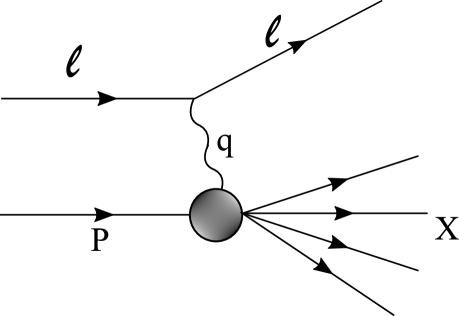
Deep inelastic scattering plays an essential role in the description of nucleon structure. In particular, to study the internal structure of a proton, one can make use of lepton-proton inelastic scattering in which an incoming lepton hits the proton and interacts with it through the exchange of a virtual photon of momentum . With energies high enough above GeV, the virtual photon can probe the internal substructure of a proton. This process is depicted in Fig. 1. The state represents the final state, which is no longer the proton.
The internal structure of a proton can be described by the hadronic tensor in four dimensions, defined as
| (1) |
where represents the electromagnetic hadronic current and the spin of the proton. In this work we are going to deal with an unpolarized target, for which the most general tensor decomposition of can be written as Manohar (1992)
| (2) |
where is the momentum fraction carried by the parton (i.e., the Bjorken parameter), and are the unpolarized DIS structure functions, with and . The lower the value of , the more inelastic the process is. The limit corresponds to the elastic regime.
Inserting a complete set of final states in (1), one can write as
| (3) |
The task is then to compute the matrix element in Eq. (3). In the following section, we describe the holographic prescription put forward by Polchinski and Strassler (2003) to perform this calculation. Later on, in Sec. VI, we proceed with the full calculation of this quantity in our Einstein-Dilaton model.
III Holographic approach for determining structure functions
As discussed in the previous section, the hadronic tensor is given in terms of the matrix element
| (4) |
To calculate (4) using holographic tools, we follow steps similar to the approach used by Polchinski and Strassler in Polchinski and Strassler (2003). The idea is to consider the matrix element above given by an interaction action defined as
| (5) |
where is the holographic coordinate, and is the coupling vertex of the photon field with the initial and final fermionic states and , involved the DIS process, respectively. All these fields live in the bulk of the five-dimensional asymptotic AdS space, and are the four-component Dirac matrices in those dimensions (see Section V.2 for details).
Polschinski and Strassler Polchinski and Strassler (2003), and other related works (see, e.g. Borsa et al. (2023); Kovensky et al. (2018a); Hatta et al. (2008); Ballon Bayona et al. (2008a, b); Cornalba and Costa (2008); Pire et al. (2008); Albacete et al. (2008); Ballon Bayona et al. (2008c); Gao and Xiao (2009); Taliotis (2009); Yoshida (2010); Hatta et al. (2009); Avsar et al. (2009); Cornalba et al. (2010a); Bayona et al. (2010); Cornalba et al. (2010b); Brower et al. (2010); Gao and Mou (2010); Ballon Bayona et al. (2010); Braga and Vega (2012); Koile et al. (2014, 2015a); Gao and Mou (2014); Folco Capossoli and Boschi-Filho (2015); Folco Capossoli et al. (2020a); Koile et al. (2015b); Jorrin et al. (2016a, b); Kovensky et al. (2018b); Amorim et al. (2018); Watanabe et al. (2020); Jorrin et al. (2020); Amorim and Costa (2021); Mamo and Zahed (2021); Tahery et al. (2023); Jorrin and Schvellinger (2022); Bigazzi and Castellani (2024); Mayrhofer (2024)) compute (5) by first solving the equations of motion for the fields, derived from actions of the form
| (6) |
where includes the probe fermionic and gauge fields, and then insert the solutions back into the matrix element in order to read off the structure functions. In previous works, the form of the asymptotic space metric was given, with properties such that some relevant QCD phenomenology could be reproduced, e.g., confinement. In this work, however, we go further and consider a new approach in this context. Instead of choosing an ad hoc particular geometry to reproduce some QCD property, we start from an Einstein-Dilaton general action involving the metric and the scalar field and solve the equations of motion for these fields to determine the bulk geometry. Once the on-shell solution for the background is known, we solve the equations for the probe fields on this background to extract the structure functions. This way, one has greater systematic control about the properties of the bulk geometry, and its regime of validity (for example, concerning its behavior near singularities Gubser (2000)). In the following section, we derive the equations of motion of the background Einstein-Dilaton model, and explain how we solve them numerically.
IV The Einstein-Dilaton model
In this section we give the details about the Einstein-Dilaton model used in this work. We follow Ref. Finazzo and Noronha (2014b), which investigated how the choice of the dilaton potential affects the Debye mass computed from Einstein-Dilaton models. The particular choice of potential used in this work corresponds to model B1 (see Sect. IV.3) in Finazzo and Noronha (2014b), which led to a good description of the tensor glueball spectrum and the thermodynamic properties of large pure Yang-Mills theory.
We start with a general Einstein-Dilaton action (with at most two derivatives) in the Einstein frame to describe the bulk
| (7) |
where , with being Newton’s constant in five dimensions. We consider here the case at zero temperature, and follow the Gubser-Nellore Ansatz Gubser and Nellore (2008) for the metric given by
| (8) |
Above, the holographic radial coordinate is given by the scalar field itself. The functions and depend on . The potential will be specified in Sect. IV.3. In the following, we will derive the equations of motion and solve them in order to determine the functions and to fully specify the background spacetime (8).
IV.1 Equations of motion
The equations of motion obtained from (7) are the Einstein field equations
| (9) |
where is the stress-energy tensor for the scalar field
| (10) |
and the equation for the scalar field is
| (11) |
Here (throughout this work primes will always denote a derivative with respect to ). Equations (9) and (11) with the metric given by (8) lead to the following equations of motion Finazzo and Noronha (2014b)
| (12) | |||
| (13) | |||
| (14) |
IV.2 Obtaining the geometry
A schematic way to obtain the geometry is done here following the master equation procedure pursued in Ref. Gubser and Nellore (2008), adapted here for the case where the temperature is zero Finazzo and Noronha (2014b). The idea is to obtain a first-order equation for and solve it to determine the functions and . Using this definition and combining equations (13) and (14), we find
| (15) |
Using (12) to eliminate from this last equation, one obtains the following
| (16) |
In order to solve (16) for a given potential , we have to specify a boundary condition for .
For the boundary conditions for , we must look at how the potential behaves in deep in the bulk () and at the boundary . To obtain a confining model, the potential must display non-analytical behavior at large , see Gursoy et al. (2008a). In our model, this requirement can be met Gubser et al. (2008b) if our potential has the following asymptotic form in the infrared
| (17) |
with being a positive real number. So, deep in the bulk we have . Eq. (16) then implies
| (18) |
At the UV boundary () the potential asymptotes to the case of a free massive scalar field plus a negative cosmological constant,
| (19) |
leading to an asymptotic AdS5 spacetime with curvature . Its UV asymptotic geometry is given by
| (20) | ||||
| (21) |
where is the UV scaling dimension of the gauge theory operator associated with . According to the holographic dictionary, this quantity is related to bulk parameters by the following relation
| (22) |
with being the mass of the scalar field in the bulk AdS5.
With all this at hand, we can obtain the functions and . Recalling that , we have
| (23) |
Also, from (12), we can write down the answer for as follows
| (24) |
Solving numerically the master equation for in Eq. (16), and then performing the required integrals to determine and , the full geometry in (8) corresponding to the on-shell solution of the Einstein-Dilaton model can be found. The last step in this direction is to choose the scalar potential to be used.
IV.3 Dilaton potential
The construction above and the choice of the scalar potential is inspired by the work in Ref. Finazzo and Noronha (2014b), where the authors use an Einstein-Dilaton model to investigate the thermodynamics and the Debye mass of pure SU() Yang-Mills theory. We use the B1 potential considered in Finazzo and Noronha (2014b), which is given by
| (25) |
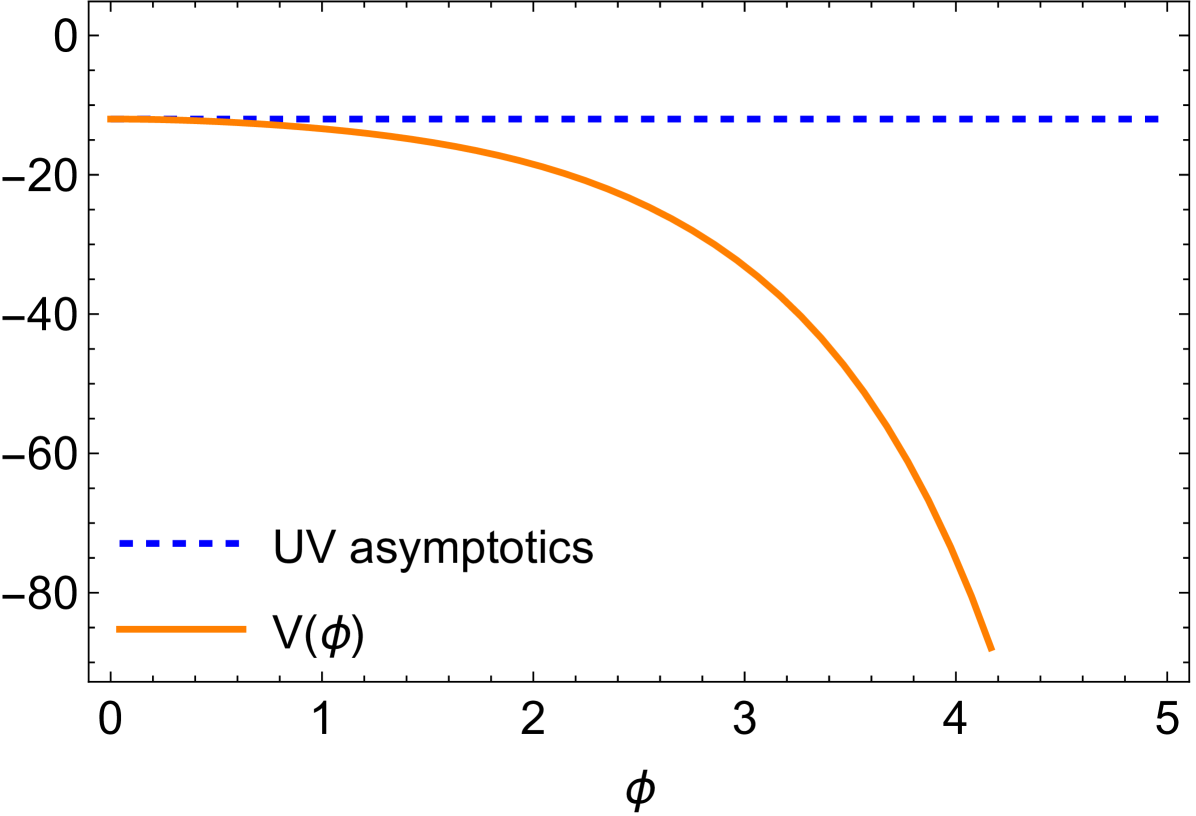
This choice of potential interpolates between the UV behavior and the IR behavior . Besides being confining at zero temperature, at finite temperature a potential with these properties implies that the gauge theory displays a first-order phase transition Gursoy et al. (2008b). The free parameters in (25) are given in Table 1 and the corresponding potential in Fig. 2.
The UV () of the effective bulk action can be extracted from Eq. (25)
| (26) |
With the values in Table 1, we obtain , which satisfies the Breitenlohner-Freedman bound Breitenlohner and Freedman (1982a, b); Mezincescu and Townsend (1985)
| (27) |
Therefore, using the AdS/CFT dictionary entry in Eq. (22), we find that the conformal dimension is . Following the reasoning laid out in Gubser et al. (2008b), we see that in this model asymptotic freedom is replaced by conformal invariance in the UV regime. Also, from now on, we use units where the AdS radius .
Although the potential in (25) was motivated by the investigation of finite temperature properties, the authors of Finazzo and Noronha (2014b) also applied it to vacuum case. In fact, in this limit, they studied the spectra of scalar , tensor , and pseudoscalar glueballs. In particular, the authors found reasonable agreement between the tensor (and axial) glueballs spectra and lattice results for pure Yang-Mills. Inspired by these results in this confining vacuum model, here we employ this zero-temperature setup to study deep inelastic scattering.
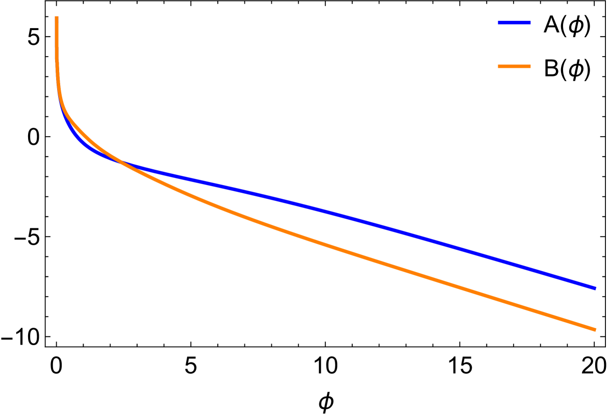
With this potential at hand one can completely determine the functions and in Eqs. (23) and (24), respectively, and use the resulting geometry to obtain the equations of motion and solutions for the fields involved in the DIS problem. This allows us to calculate the hadronic tensor and predict in this configuration. The numerical solution for the profiles of and that determine the metric, with the parameters fixed in Table 1, are presented in Fig. 3. We have checked that we recover the results originally shown in Finazzo and Noronha (2014b).
V Probe Fields
In the DIS process, the particles involved are probe fields in the bulk geometry we have obtained in the last section. We now proceed to obtain their equations of motion. This is done considering the actions for each field, separately.
V.1 Virtual photon field
The virtual photon is described by the following action
| (28) |
with
| (29) |
The equations of motion from the action (28) are
| (30) |
where
| (31) |
The case leads to the following equations
| (32) | |||
| (33) |
while the case leads to
| (34) |
which implies
| (35) | ||||
| (36) |
Using the gauge-fixing
| (37) |
along with (35) and (36), one can write (32) as
| (38) |
Furthermore, we will consider a photon with a particular polarization such that . In this case, only the components will contribute to the scattering process, disregarding . Thus, we just have to solve Eq. (38) for the virtual photon. Also, by imposing the boundary condition,
| (39) |
we shall consider solutions of the form
| (40) |
Inserting (40) into Eq. (38), we find the following equation of motion for
| (41) |
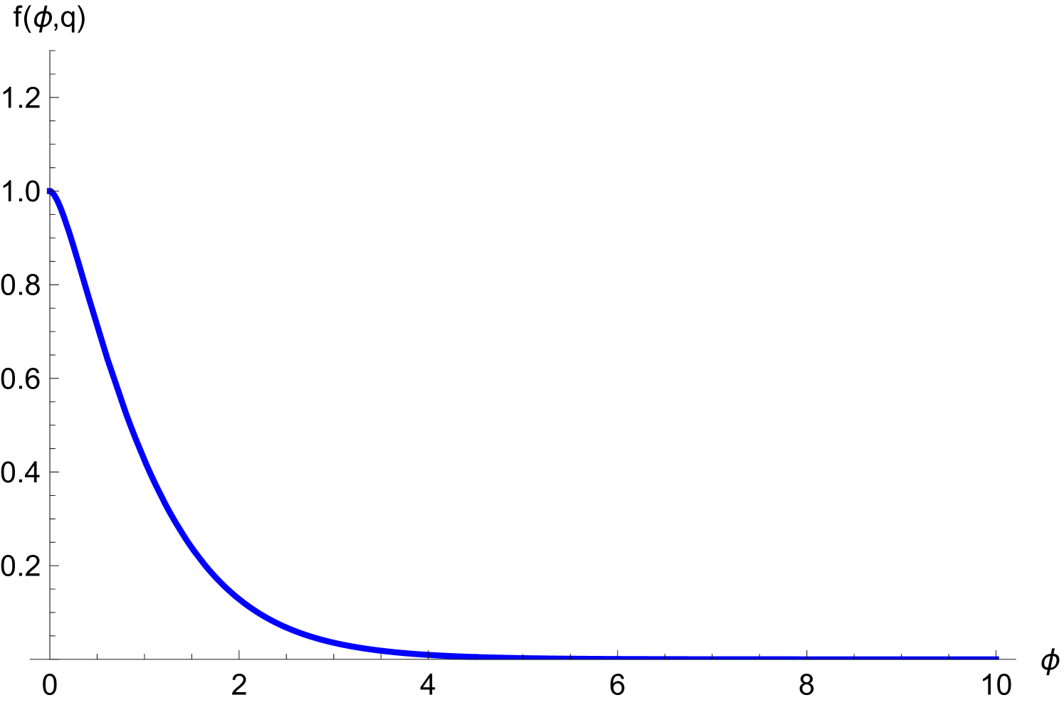
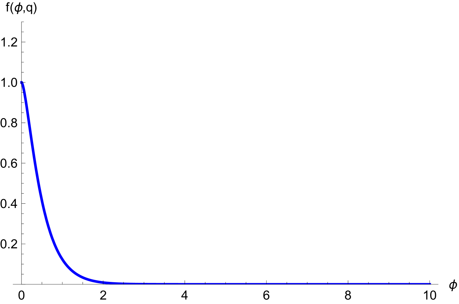
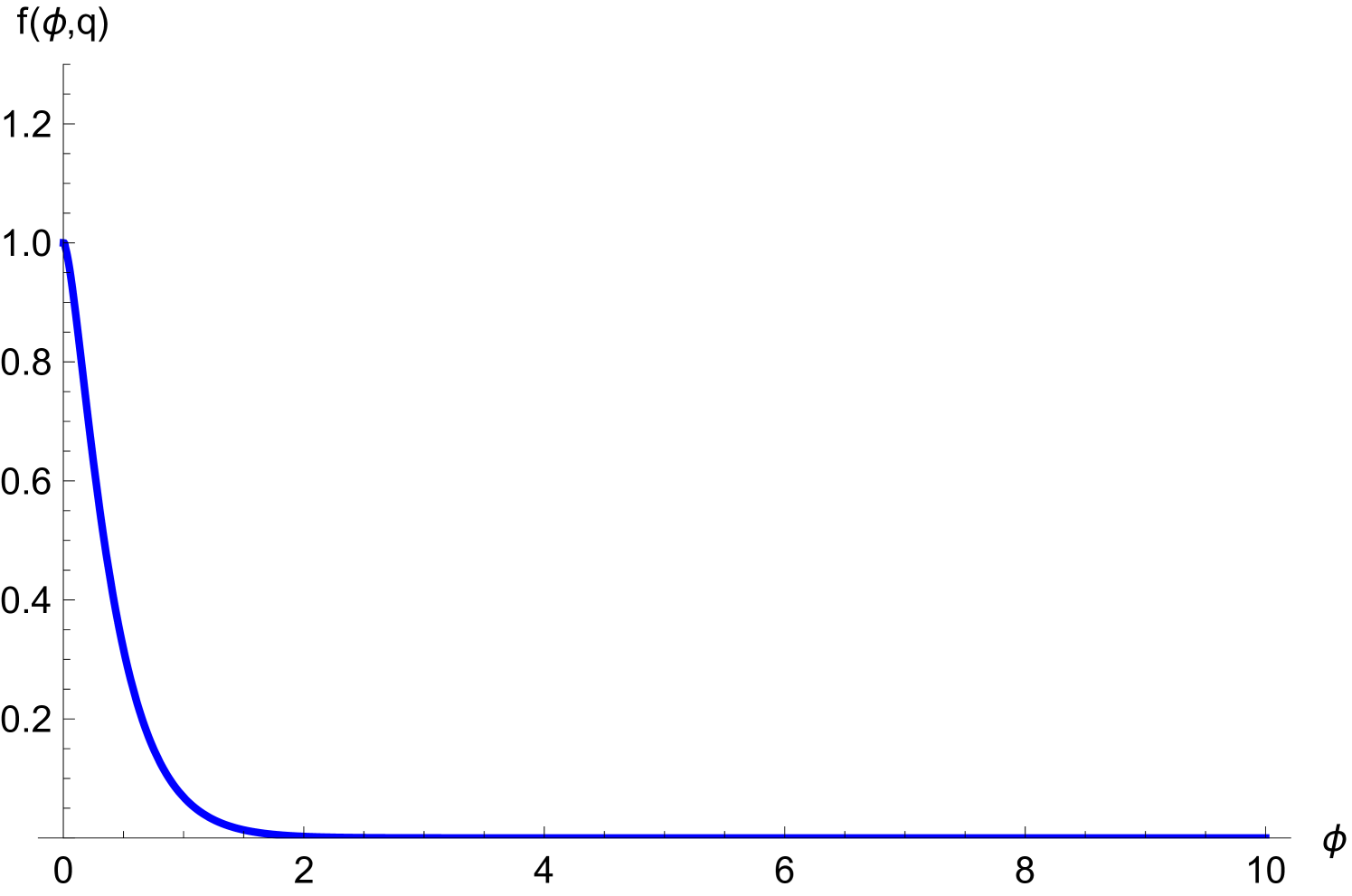
This equation will be solved numerically for , with and given as in the previous section, to determine the virtual photon profile in this model. The result is displayed in Fig. 4.
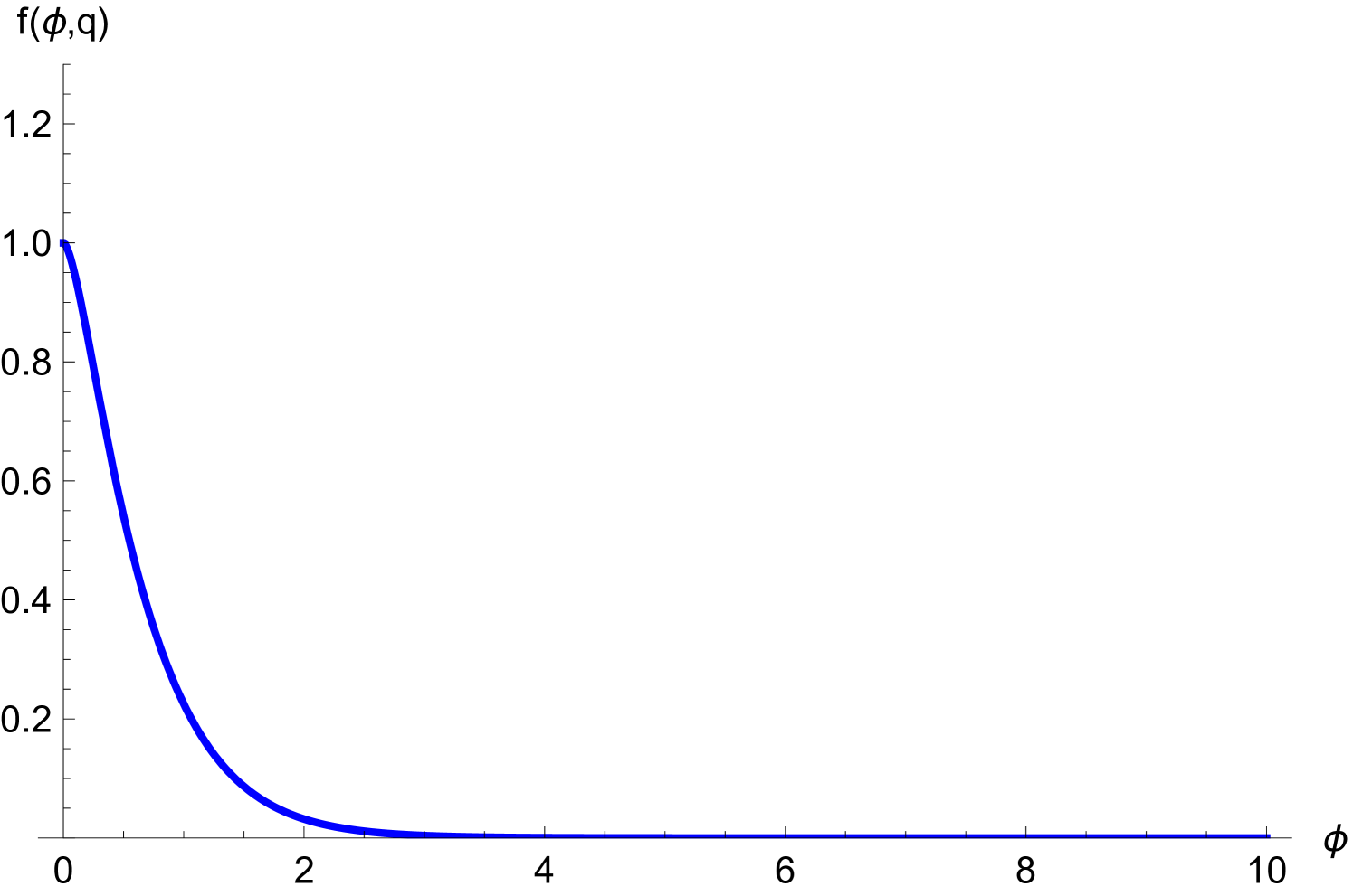
It is also possible to obtain approximate analytical solutions for the photon field. First, if we consider the limit , then, with , the functions and both reduce to , so that , in this limit. The solution in the case is
| (42) |
which is nicely written in terms of Bessel functions of the first and second kind. This is just the solution in pure AdS5, as expected. Note that this solution heavily depends on the sign of , which defines the virtuality of the photon. In the opposite case, , one finds
| (43) |
Thus, we see that solution in Eq. (42) is a sum of monotonically increasing and decreasing functions, while the solution (43) is oscillatory.
Going further in the approximation for the functions and , now including the contribution of linear terms, one finds
| (44) | |||||
| (45) |
where and , as can be extracted from Fig. 3, corresponding to the values of the functions and with the parameters given in Table 1. Substituting the expressions for and given by Eqs. (44) and (45) into equation (41), one finds the general solution for , , and :
| (46) |
where and are arbitrary constants to be fixed by boundary conditions, while and are the confluent hypergeometric function of the second kind and the associated Laguerre function, respectively. Above, we defined the constants
| (47) | |||||
| (48) | |||||
| (49) |
Note that for any , so that , and , implying decreasing exponential factors in both terms in Eq. (46). This behavior is clearly found in Fig. 4 for some values of , including the case , for which a particular solution of Eq. (41) can be also found.
V.2 Baryonic states
The fermionic fields representing the initial and final hadrons are described by the action
| (50) |
where represents a spin 1/2 field with mass in five-dimensional space, and is the five-dimensional Dirac operator defined as:
| (51) |
where again prime denotes derivative with respect to , and the Dirac matrices , with , , and following the convention of Refs. Henningson and Sfetsos (1998); Mueck and Viswanathan (1998); Kirsch (2006); Abidin and Carlson (2009). The indices represent curved spacetime labels, referring to the coordinates in the bulk geometry. represent the quantities of the locally flat tangent space, while represent the Minkowski space indices. Thus, the vielbein are given by:
| (52) |
where the fifth coordinate is the radial coordinate .
For the spin connection , one finds
| (53) |
where the Christoffel symbols are written as:
| (54) |
The only non-vanishing for the asymptotic AdS5 space are
| (55) |
so that
| (56) |
and all other components of the spin connection vanish. Then, the Dirac operator becomes
| (57) |
From the action (50), one can derive the five-dimensional Dirac equations of motion
| (58) |
which can be written as follows
| (59) |
The four-component Dirac spinor defined in the bulk of the five-dimensional space can be decomposed into left- and right-handed chiral components as:
| (60) |
where
| (61) |
Since , the following relations hold
| (62) | ||||
| (63) |
where is the four-dimensional fermionic mass.
Assuming the Kaluza-Klein modes are dual to the chiral spinors, we have
| (64) |
Now, using (64) along with (60) into (59), we arrive at the following set of coupled equations
| (65) | ||||
| (66) |
where are the discrete four dimensional fermionic masses with .
In order to decouple Eqs. (65) and (66), one takes the second derivative with respect to and obtains
| (67) |
From (65) and (66), we can solve for and
| (68) | ||||
| (69) |
Substituting (69) into (68), one finds
| (70) |
Now we have equations (70), (65), and (66) for and , respectively. Inserting these three equations into (67), one obtains
| (71) |
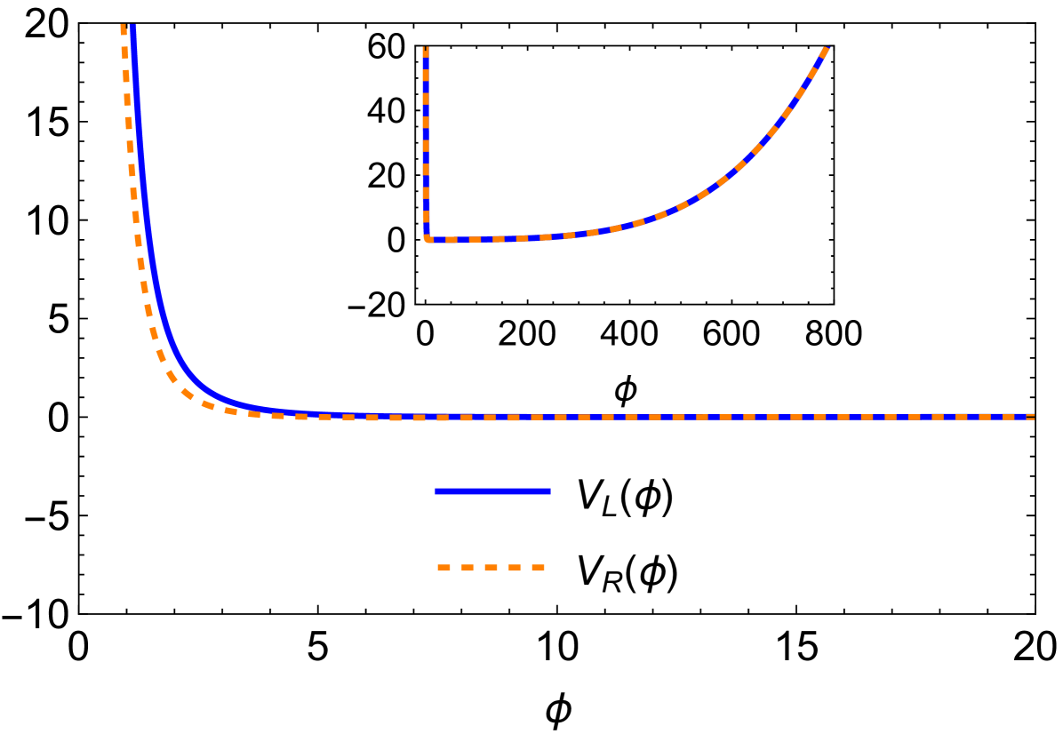
Finally, performing the following transformation
| (72) |
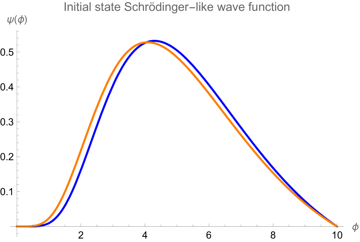
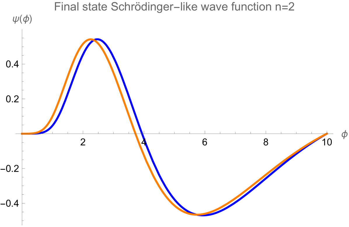
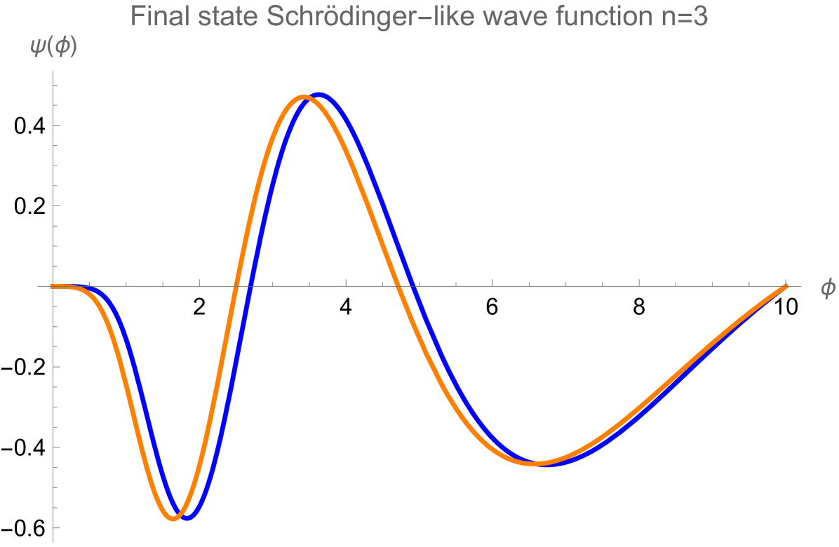
one arrives at a Schrödinger-like equation for
| (73) |
with the right and left potentials given by
| (74) |
These potentials are shown in Figure 7 for the set of parameters defined in Table 1, corresponding to the numerically obtained metric functions and , shown in Fig. 3.
Then, we can write the initial and final baryonic states as linear combinations of solutions :
| (75) | ||||
| (76) |
Before we move on to compute the interaction action, we comment on the role of adding an anomalous dimension to this problem. When solving Eq. (73), we want to fix the ground state to be the proton. According to the holographic dictionary, the bulk fermionic mass is related to the canonical scaling dimension of a fermionic operator at the boundary by the following:
| (77) |
For , we consider the initial state of our problem to be the proton, and regard it as single particle. This choice will be justified by the results we get for for large values of the transferred momentum. Then, we take , the canonical scaling dimension for fermions. However, this procedure does not reproduce the proton mass as the initial state of the eigenvalue problem. Phenomenologically, it is necessary to consider an anomalous dimension to fit the exact value of the proton mass. We thus solve the Schrödinger-like equation (73) considering
| (78) |
By choosing an appropriate , we can obtain the proton mass as the ground state for one of the chiral solutions, as shown in Table 2.
VI The DIS interaction action
In this section, we will explicitly compute the DIS interaction action in Eq. (5), repeated here for convenience
| (79) |
Using the definitions of the vielbein given by Eqs. (52) and (54), associated with the geometry of the metric (8), one can rewrite the interaction action , disregarding the component as discussed in Sect. V.1, as follows
| (80) | |||||
The initial and final spinor states, and , are given, respectively, by Eqs. (75) and (76). We also note that
| (81) |
With these results and the gauge field given by Eq. (40), using , we can write the interaction action as follows,
| (83) |
where the are defined in terms of the solutions of the chiral fermions and the solution of the photon field , so that
| (84) |
From Eqs. (5) and (83), one finds
| (85) | |||||
| (86) | |||||
where is an effective coupling constant related to . Contracting the photon polarization with the hadronic tensor, Eq. (5), one obtains
| (87) | |||||
where is the mass of the final hadronic state. As we are interested in a spin-independent scenario, using the following property, we perform a summation over spin, so that
| (88) |
Thus, one finds
| (89) | |||||
where is the fermionic ground state mass that we identify with that of the proton. Applying some trace engineering in Eq. (89), we obtain
| (90) |
In order to obtain the expression for the structure function , we need to sum over the outgoing states , as presented in Eq. (3). Carrying on this sum to the continuum limit, we can evaluate the invariant mass delta function. Following Ref. Polchinski and Strassler (2003), this integration will be related to the functional form of the mass spectrum of the produced particles with the excitation number ,
that for the soft and hard wall models accounts for the lowest state produced at the collision, since the spectrum is linear with Polchinski and Strassler (2003); Ballon Bayona et al. (2008b). In our case, this delta will account for .
Taking into account our choice of transversal polarization (), the hadronic tensor has the following form
| (91) |
From this equation, one can explicitly construct the baryonic DIS structure functions. We find
| (92) | |||||
| (93) |
where the hadronic masses of the initial and final states, and , respectively, are related by
| (94) |
Note that from Eqs. (92) and (93), the two structure functions and are related by
| (95) |
so that, in the limit of and , with , one finds
| (96) |
which recovering the Callan-Gross relation , for , as expected from the model’s asymptotic conformal invariance. Finally, we note that the ratio between the structure functions does not depend on the parameter , though it would still depend on the anomalous dimension .
VII Results
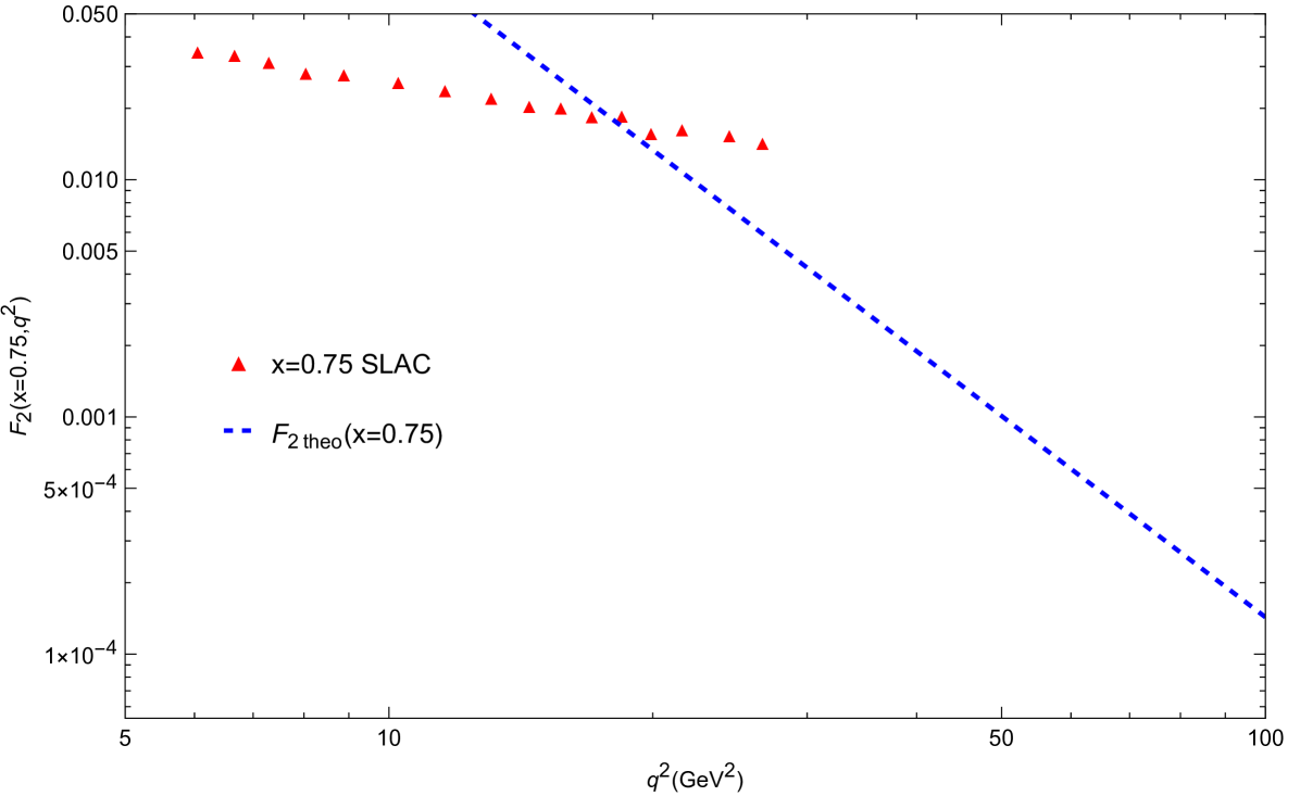
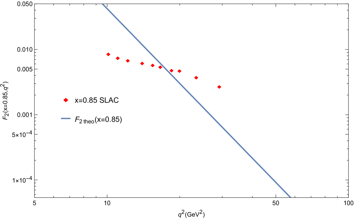
In this section, we show the numerical results for the structure function as a function of for two different values of the Bjorken parameter: and . These are the largest values of measured for Whitlow et al. (1992). The kinematical range for considered above is near the elastic regime ( close to ). In this large domain, it is reasonable to consider the scattering off the entire proton rather than by its constituent partons.
In our analysis of DIS in terms of the probe fields, there are two free parameters involved: and . The effective coupling constant controls the overall magnitude of obtained from Eq. (93). One can then adjust it so that our crosses the data at least at a single point. The anomalous dimension is chosen so that the solutions to Eqs. (73) fit the proton mass in the initial state. These values are displayed in Tables 2 and 3. In addition to that, we also show in Table 2 the values for the ground state masses of the left-chiral and right-chiral fermions, and , respectively, resulting from this choice of . Notice that the right-chiral fermion fits the proton mass , with the left-chiral mass having a different and higher value. For this reason, we take the right chiral solution to represent the initial state of the scattering process.
Our results for and as functions of are shown in Fig. 8. We note that we chose two values of , one for each , though only a single value of was used. With this simple setup, one can make our calculations for to have reasonable values, staying relatively close to the experimental data. More importantly, the model qualitatively reproduces the general trend displayed by which decreases with increasing values, being thus consistent with the interpretation of scattering off the entire proton at large .
VIII Conclusions
In this work, we presented a framework for computing proton structure functions in a general class of Einstein-Dilaton holographic models. Our approach is valid for any choice of the dilaton potential . Different than previous works, the background geometry is determined from a well-defined bulk action, which leads to equations of motion that can be numerically solved to determine the on-shell profiles of the metric and dilaton fields. Following Polchinski and Strassler, we introduce probe gauge and fermionic fields to discuss DIS from a holographic perspective. Using the metric and scalar fields self-consistently obtained from the Einstein-Dilaton model, one can then solve the corresponding equations of motion for the probe fields. With that information at hand, the structure functions can be directly computed. Therefore, from our framework, the dependence of the proton structure functions on and follow from the choices made for the dilaton potential , and the parameters and associated with the probe fields.
As an application, we use a particular realization of the Einstein-Dilaton model with a constructed in such a way that the model displays linear confinement and quantitatively describes the glueball spectrum at zero temperature, in addition to describing the thermodynamic properties of deconfined large pure Yang-Mills theory. In this case, all the parameters that define the background are fixed using QCD input that is not connected to DIS physics.
We solved the equations of motion for the probe fields in this specific background, making choices for the probe field parameters and . We were able to successfully fit the initial state proton mass within this model and, as one can see in Table 2, the initial proton masses for the left and right chiral fermions are close to the actual value of GeV, especially . However, as one can see from Fig. 8, this particular realization of the model does not quantitatively reproduce the experimental data for . Nevertheless, we note that we find the same general qualitative behavior, i.e., a decreasing with increasing , displayed by other holographic models that were tailored for describing in the same range of Bjorken considered here Braga and Vega (2012); Folco Capossoli et al. (2020a).
This provides a nice example of the limitations of holographic approaches when it comes to QCD modeling. This is expected, of course, since these models are not QCD. Each holographic model may capture some individual aspects of quantum chromodynamics which one is interested in. For example, using a different holographic model and a different warp factor in the background geometry that was not obtained from an action, the authors of Folco Capossoli et al. (2020a) calculate and fit to experimental data for a particular choice of the parameters that appear in their model. However, in Folco Capossoli et al. (2020b), a completely different choice of the same parameters is used in the same model to describe the masses of glueballs, scalars, and vector mesons found on the lattice. Thus, the parameters in that model differ depending on the problem at hand. In this paper, we work towards a more self-consistent approach as we keep the of the Einstein-Dilaton model fixed, so that the model describes some relevant non-DIS related properties of QCD, and then show this still allows us to reproduce some general features of deep inelastic scattering.
In principle, a quantitative description of the data should be possible in our framework by performing a combined Bayesian inference analysis to obtain optimal model parameters that can fit multiple observables at once, constructing a family of results. In this regard, we note that Bayesian methods have been used in similar holographic models already in Hippert et al. (2024). We leave this interesting possibility for future work.
Acknowledgments
A.C.P.N. thanks Adão Silva and Leonardo Pazito for their valuable comments on the making of this work. He is supported by Coordenação de Aperfeiçoamento de Pessoal de Nível Superior (CAPES), and also acknowledges the hospitality extended to him at the Illinois Center for Advanced Studies of the Universe & Department of Physics, University of Illinois Urbana-Champaign, during his stay from April through September of 2024, supported by the CAPES PrInt program. H.B.-F. is partially supported by Conselho Nacional de Desenvolvimento Científico e Tecnológico (CNPq) under grant 310346/2023-1, and Fundação Carlos Chagas Filho de Amparo à Pesquisa do Estado do Rio de Janeiro (FAPERJ) under grant E-26/204.095/2024. J.N. was partially supported by the U.S. Department of Energy, Office of Science, Office for Nuclear Physics under Award No. DESC0023861. This research was partially supported by the National Science Foundation under grant No. NSF PHY-1748958.
References
- Breidenbach et al. (1969) M. Breidenbach, J. I. Friedman, H. W. Kendall, E. D. Bloom, D. H. Coward, H. C. DeStaebler, J. Drees, L. W. Mo, and R. E. Taylor, Phys. Rev. Lett. 23, 935 (1969).
- Bloom et al. (1969) E. D. Bloom et al., Phys. Rev. Lett. 23, 930 (1969).
- Whitlow et al. (1992) L. W. Whitlow, E. M. Riordan, S. Dasu, S. Rock, and A. Bodek, Phys. Lett. B 282, 475 (1992).
- Gross and Wilczek (1973) D. J. Gross and F. Wilczek, Phys. Rev. Lett. 30, 1343 (1973).
- Politzer (1973) H. D. Politzer, Phys. Rev. Lett. 30, 1346 (1973).
- Dokshitzer (1977) Y. L. Dokshitzer, Sov. Phys. JETP 46, 641 (1977).
- Gribov and Lipatov (1972) V. N. Gribov and L. N. Lipatov, Sov. J. Nucl. Phys. 15, 438 (1972).
- Altarelli and Parisi (1977) G. Altarelli and G. Parisi, Nucl. Phys. B 126, 298 (1977).
- Gross et al. (1977) D. J. Gross, S. B. Treiman, and F. A. Wilczek, Phys. Rev. D 15, 2486 (1977).
- Jaroszewicz (1982) T. Jaroszewicz, Phys. Lett. B 116, 291 (1982).
- Manohar (1992) A. V. Manohar, in Lake Louise Winter Institute: Symmetry and Spin in the Standard Model (1992) arXiv:hep-ph/9204208 .
- Gelis et al. (2010) F. Gelis, E. Iancu, J. Jalilian-Marian, and R. Venugopalan, Ann. Rev. Nucl. Part. Sci. 60, 463 (2010), arXiv:1002.0333 [hep-ph] .
- Accardi et al. (2016) A. Accardi et al., Eur. Phys. J. A 52, 268 (2016), arXiv:1212.1701 [nucl-ex] .
- Habib (2010) S. Habib (H1, ZEUS), PoS DIS2010, 035 (2010).
- Maldacena (1998) J. M. Maldacena, Adv. Theor. Math. Phys. 2, 231 (1998), arXiv:hep-th/9711200 .
- Gubser et al. (1998) S. S. Gubser, I. R. Klebanov, and A. M. Polyakov, Phys. Lett. B 428, 105 (1998), arXiv:hep-th/9802109 .
- Witten (1998) E. Witten, Adv. Theor. Math. Phys. 2, 253 (1998), arXiv:hep-th/9802150 .
- Aharony et al. (2000) O. Aharony, S. S. Gubser, J. M. Maldacena, H. Ooguri, and Y. Oz, Phys. Rept. 323, 183 (2000), arXiv:hep-th/9905111 .
- Gubser et al. (2002) S. S. Gubser, I. R. Klebanov, and A. M. Polyakov, Nucl. Phys. B 636, 99 (2002), arXiv:hep-th/0204051 .
- Polchinski and Strassler (2003) J. Polchinski and M. J. Strassler, JHEP 05, 012 (2003), arXiv:hep-th/0209211 .
- Borsa et al. (2023) I. Borsa, D. Jorrin, R. Sassot, and M. Schvellinger, Phys. Rev. D 108, 056024 (2023), arXiv:2308.01975 [hep-ph] .
- Kovensky et al. (2018a) N. Kovensky, G. Michalski, and M. Schvellinger, JHEP 10, 084 (2018a), arXiv:1807.11540 [hep-th] .
- Hatta et al. (2008) Y. Hatta, E. Iancu, and A. H. Mueller, JHEP 01, 026 (2008), arXiv:0710.2148 [hep-th] .
- Ballon Bayona et al. (2008a) C. A. Ballon Bayona, H. Boschi-Filho, and N. R. F. Braga, JHEP 10, 088 (2008a), arXiv:0712.3530 [hep-th] .
- Ballon Bayona et al. (2008b) C. A. Ballon Bayona, H. Boschi-Filho, and N. R. F. Braga, JHEP 03, 064 (2008b), arXiv:0711.0221 [hep-th] .
- Cornalba and Costa (2008) L. Cornalba and M. S. Costa, Phys. Rev. D 78, 096010 (2008), arXiv:0804.1562 [hep-ph] .
- Pire et al. (2008) B. Pire, C. Roiesnel, L. Szymanowski, and S. Wallon, Phys. Lett. B 670, 84 (2008), arXiv:0805.4346 [hep-ph] .
- Albacete et al. (2008) J. L. Albacete, Y. V. Kovchegov, and A. Taliotis, JHEP 07, 074 (2008), arXiv:0806.1484 [hep-th] .
- Ballon Bayona et al. (2008c) C. A. Ballon Bayona, H. Boschi-Filho, and N. R. F. Braga, JHEP 09, 114 (2008c), arXiv:0807.1917 [hep-th] .
- Gao and Xiao (2009) J.-H. Gao and B.-W. Xiao, Phys. Rev. D 80, 015025 (2009), arXiv:0904.2870 [hep-ph] .
- Taliotis (2009) A. Taliotis, Nucl. Phys. A 830, 299C (2009), arXiv:0907.4204 [hep-th] .
- Yoshida (2010) Y. Yoshida, Prog. Theor. Phys. 123, 79 (2010), arXiv:0902.1015 [hep-th] .
- Hatta et al. (2009) Y. Hatta, T. Ueda, and B.-W. Xiao, JHEP 08, 007 (2009), arXiv:0905.2493 [hep-ph] .
- Avsar et al. (2009) E. Avsar, E. Iancu, L. McLerran, and D. N. Triantafyllopoulos, JHEP 11, 105 (2009), arXiv:0907.4604 [hep-th] .
- Cornalba et al. (2010a) L. Cornalba, M. S. Costa, and J. Penedones, JHEP 03, 133 (2010a), arXiv:0911.0043 [hep-th] .
- Bayona et al. (2010) C. A. B. Bayona, H. Boschi-Filho, and N. R. F. Braga, Phys. Rev. D 81, 086003 (2010), arXiv:0912.0231 [hep-th] .
- Cornalba et al. (2010b) L. Cornalba, M. S. Costa, and J. Penedones, Phys. Rev. Lett. 105, 072003 (2010b), arXiv:1001.1157 [hep-ph] .
- Brower et al. (2010) R. C. Brower, M. Djuric, I. Sarcevic, and C.-I. Tan, JHEP 11, 051 (2010), arXiv:1007.2259 [hep-ph] .
- Gao and Mou (2010) J.-H. Gao and Z.-G. Mou, Phys. Rev. D 81, 096006 (2010), arXiv:1003.3066 [hep-ph] .
- Ballon Bayona et al. (2010) C. A. Ballon Bayona, H. Boschi-Filho, N. R. F. Braga, and M. A. C. Torres, JHEP 10, 055 (2010), arXiv:1007.2448 [hep-th] .
- Braga and Vega (2012) N. R. F. Braga and A. Vega, Eur. Phys. J. C 72, 2236 (2012), arXiv:1110.2548 [hep-ph] .
- Koile et al. (2014) E. Koile, S. Macaluso, and M. Schvellinger, JHEP 01, 166 (2014), arXiv:1311.2601 [hep-th] .
- Koile et al. (2015a) E. Koile, N. Kovensky, and M. Schvellinger, JHEP 05, 001 (2015a), arXiv:1412.6509 [hep-th] .
- Gao and Mou (2014) J.-H. Gao and Z.-G. Mou, Phys. Rev. D 90, 075018 (2014), arXiv:1406.7576 [hep-ph] .
- Folco Capossoli and Boschi-Filho (2015) E. Folco Capossoli and H. Boschi-Filho, Phys. Rev. D 92, 126012 (2015), arXiv:1509.01761 [hep-th] .
- Folco Capossoli et al. (2020a) E. Folco Capossoli, M. A. Martín Contreras, D. Li, A. Vega, and H. Boschi-Filho, Phys. Rev. D 102, 086004 (2020a), arXiv:2007.09283 [hep-ph] .
- Koile et al. (2015b) E. Koile, N. Kovensky, and M. Schvellinger, JHEP 12, 009 (2015b), arXiv:1507.07942 [hep-th] .
- Jorrin et al. (2016a) D. Jorrin, N. Kovensky, and M. Schvellinger, JHEP 04, 113 (2016a), arXiv:1601.01627 [hep-th] .
- Jorrin et al. (2016b) D. Jorrin, M. Schvellinger, and N. Kovensky, JHEP 12, 003 (2016b), arXiv:1609.01202 [hep-th] .
- Kovensky et al. (2018b) N. Kovensky, G. Michalski, and M. Schvellinger, JHEP 04, 118 (2018b), arXiv:1711.06171 [hep-th] .
- Amorim et al. (2018) A. Amorim, R. Carcassés Quevedo, and M. S. Costa, Phys. Rev. D 98, 026016 (2018), arXiv:1804.07778 [hep-ph] .
- Watanabe et al. (2020) A. Watanabe, T. Sawada, and M. Huang, Phys. Lett. B 805, 135470 (2020), arXiv:1910.10008 [hep-ph] .
- Jorrin et al. (2020) D. Jorrin, G. Michalski, and M. Schvellinger, JHEP 06, 063 (2020), arXiv:2004.02909 [hep-th] .
- Amorim and Costa (2021) A. Amorim and M. S. Costa, Phys. Rev. D 103, 026007 (2021).
- Mamo and Zahed (2021) K. A. Mamo and I. Zahed, Phys. Rev. D 104, 066010 (2021), arXiv:2102.00608 [hep-ph] .
- Tahery et al. (2023) S. Tahery, X. Wang, and X. Chen, Chin. Phys. C 47, 013101 (2023), arXiv:2111.06616 [hep-ph] .
- Jorrin and Schvellinger (2022) D. Jorrin and M. Schvellinger, Phys. Rev. D 106, 066024 (2022), arXiv:2207.02984 [hep-ph] .
- Bigazzi and Castellani (2024) F. Bigazzi and F. Castellani, JHEP 04, 037 (2024), arXiv:2308.16833 [hep-ph] .
- Mayrhofer (2024) C. Mayrhofer, Deep Inelastic Scattering and the WSS Model: A Study of Holographic Pomeron Exchange, Ph.D. thesis, Vienna, Tech. U. (2024).
- Gursoy and Kiritsis (2008) U. Gursoy and E. Kiritsis, JHEP 02, 032 (2008), arXiv:0707.1324 [hep-th] .
- Gursoy et al. (2008a) U. Gursoy, E. Kiritsis, and F. Nitti, JHEP 02, 019 (2008a), arXiv:0707.1349 [hep-th] .
- Erlich et al. (2005) J. Erlich, E. Katz, D. T. Son, and M. A. Stephanov, Phys. Rev. Lett. 95, 261602 (2005), arXiv:hep-ph/0501128 .
- Karch et al. (2006) A. Karch, E. Katz, D. T. Son, and M. A. Stephanov, Phys. Rev. D 74, 015005 (2006), arXiv:hep-ph/0602229 .
- Ballon-Bayona et al. (2018) A. Ballon-Bayona, H. Boschi-Filho, L. A. H. Mamani, A. S. Miranda, and V. T. Zanchin, Phys. Rev. D 97, 046001 (2018), arXiv:1708.08968 [hep-th] .
- Ballon-Bayona et al. (2023) A. Ballon-Bayona, T. Frederico, L. A. H. Mamani, and W. de Paula, Phys. Rev. D 108, 106016 (2023), arXiv:2308.07503 [hep-ph] .
- Ballon-Bayona and Junior (2024) A. Ballon-Bayona and A. a. S. d. S. Junior, Phys. Rev. D 109, 094050 (2024), arXiv:2402.17950 [hep-ph] .
- Gursoy et al. (2009) U. Gursoy, E. Kiritsis, L. Mazzanti, and F. Nitti, JHEP 05, 033 (2009), arXiv:0812.0792 [hep-th] .
- Gursoy et al. (2008b) U. Gursoy, E. Kiritsis, L. Mazzanti, and F. Nitti, Phys. Rev. Lett. 101, 181601 (2008b), arXiv:0804.0899 [hep-th] .
- Gubser and Nellore (2008) S. S. Gubser and A. Nellore, Phys. Rev. D 78, 086007 (2008), arXiv:0804.0434 [hep-th] .
- Gubser et al. (2008a) S. S. Gubser, A. Nellore, S. S. Pufu, and F. D. Rocha, Phys. Rev. Lett. 101, 131601 (2008a), arXiv:0804.1950 [hep-th] .
- Gubser et al. (2008b) S. S. Gubser, S. S. Pufu, and F. D. Rocha, JHEP 08, 085 (2008b), arXiv:0806.0407 [hep-th] .
- Noronha (2010) J. Noronha, Phys. Rev. D 81, 045011 (2010), arXiv:0910.1261 [hep-th] .
- Gursoy et al. (2011) U. Gursoy, E. Kiritsis, L. Mazzanti, G. Michalogiorgakis, and F. Nitti, Lect. Notes Phys. 828, 79 (2011), arXiv:1006.5461 [hep-th] .
- Finazzo and Noronha (2014a) S. I. Finazzo and J. Noronha, Phys. Rev. D 89, 106008 (2014a), arXiv:1311.6675 [hep-th] .
- Finazzo and Noronha (2014b) S. I. Finazzo and J. Noronha, Phys. Rev. D 90, 115028 (2014b), arXiv:1411.4330 [hep-th] .
- DeWolfe et al. (2011a) O. DeWolfe, S. S. Gubser, and C. Rosen, Phys. Rev. D 83, 086005 (2011a), arXiv:1012.1864 [hep-th] .
- DeWolfe et al. (2011b) O. DeWolfe, S. S. Gubser, and C. Rosen, Phys. Rev. D 84, 126014 (2011b), arXiv:1108.2029 [hep-th] .
- Rougemont et al. (2016) R. Rougemont, A. Ficnar, S. Finazzo, and J. Noronha, JHEP 04, 102 (2016), arXiv:1507.06556 [hep-th] .
- Rougemont et al. (2015) R. Rougemont, J. Noronha, and J. Noronha-Hostler, Phys. Rev. Lett. 115, 202301 (2015), arXiv:1507.06972 [hep-ph] .
- Critelli et al. (2017) R. Critelli, J. Noronha, J. Noronha-Hostler, I. Portillo, C. Ratti, and R. Rougemont, Phys. Rev. D 96, 096026 (2017), arXiv:1706.00455 [nucl-th] .
- Ballon-Bayona et al. (2020) A. Ballon-Bayona, H. Boschi-Filho, E. F. Capossoli, and D. M. Rodrigues, Phys. Rev. D 102, 126003 (2020), arXiv:2006.08810 [hep-th] .
- Grefa et al. (2021) J. Grefa, J. Noronha, J. Noronha-Hostler, I. Portillo, C. Ratti, and R. Rougemont, Phys. Rev. D 104, 034002 (2021), arXiv:2102.12042 [nucl-th] .
- Grefa et al. (2022) J. Grefa, M. Hippert, J. Noronha, J. Noronha-Hostler, I. Portillo, C. Ratti, and R. Rougemont, Phys. Rev. D 106, 034024 (2022), arXiv:2203.00139 [nucl-th] .
- Hippert et al. (2024) M. Hippert, J. Grefa, T. A. Manning, J. Noronha, J. Noronha-Hostler, I. Portillo Vazquez, C. Ratti, R. Rougemont, and M. Trujillo, Phys. Rev. D 110, 094006 (2024), arXiv:2309.00579 [nucl-th] .
- Rougemont et al. (2024) R. Rougemont, J. Grefa, M. Hippert, J. Noronha, J. Noronha-Hostler, I. Portillo, and C. Ratti, Prog. Part. Nucl. Phys. 135, 104093 (2024), arXiv:2307.03885 [nucl-th] .
- Jarvinen and Kiritsis (2012) M. Jarvinen and E. Kiritsis, JHEP 03, 002 (2012), arXiv:1112.1261 [hep-ph] .
- Deng and Hou (2025) J. Deng and D. Hou, (2025), arXiv:2502.00771 [nucl-th] .
- Lucini and Teper (2001) B. Lucini and M. Teper, JHEP 06, 050 (2001), arXiv:hep-lat/0103027 .
- Lucini et al. (2010) B. Lucini, A. Rago, and E. Rinaldi, JHEP 08, 119 (2010), arXiv:1007.3879 [hep-lat] .
- Panero (2009) M. Panero, Phys. Rev. Lett. 103, 232001 (2009), arXiv:0907.3719 [hep-lat] .
- Gubser (2000) S. S. Gubser, Adv. Theor. Math. Phys. 4, 679 (2000), arXiv:hep-th/0002160 .
- Breitenlohner and Freedman (1982a) P. Breitenlohner and D. Z. Freedman, Phys. Lett. B 115, 197 (1982a).
- Breitenlohner and Freedman (1982b) P. Breitenlohner and D. Z. Freedman, Annals Phys. 144, 249 (1982b).
- Mezincescu and Townsend (1985) L. Mezincescu and P. K. Townsend, Annals Phys. 160, 406 (1985).
- Henningson and Sfetsos (1998) M. Henningson and K. Sfetsos, Phys. Lett. B 431, 63 (1998), arXiv:hep-th/9803251 .
- Mueck and Viswanathan (1998) W. Mueck and K. S. Viswanathan, Phys. Rev. D 58, 106006 (1998), arXiv:hep-th/9805145 .
- Kirsch (2006) I. Kirsch, JHEP 09, 052 (2006), arXiv:hep-th/0607205 .
- Abidin and Carlson (2009) Z. Abidin and C. E. Carlson, Phys. Rev. D 79, 115003 (2009), arXiv:0903.4818 [hep-ph] .
- Folco Capossoli et al. (2020b) E. Folco Capossoli, M. A. Martín Contreras, D. Li, A. Vega, and H. Boschi-Filho, Chin. Phys. C 44, 064104 (2020b), arXiv:1903.06269 [hep-ph] .