Provable Membership Inference Privacy

We make use of the following notation. We will use $\mathcal{D}$ to refer to our entire dataset, which consists of $n$ samples all of which must remain private. We will use $\mathbf{x}\in\mathcal{D}$ or $\mathbf{x}^{*}\in\mathcal{D}$ to refer to a particular sample. $\mathcal{D}_{\mathrm{train}}\subseteq\mathcal{D}$ refers to a size-$k$ subset of $\mathcal{D}$. We will assume the subset is selected randomly, so $\mathcal{D}_{\mathrm{train}}$ is a random variable. The remaining data $\mathcal{D}\setminus\mathcal{D}_{\mathrm{train}}$ will be referred to as the holdout data. We denote by $\mathbb{D}$ the set of all size-$k$ subsets of $\mathcal{D}$ (i.e., all possible training sets), and we will use $D\in\mathbb{D}$ to refer to a particular realization of the random variable $\mathcal{D}_{\mathrm{train}}$. Finally, given a particular sample $\mathbf{x}^{*}\in\mathcal{D}$, $\mathbb{D}^{\mathrm{in}}$ (resp. $\mathbb{D}^{\mathrm{out}}$) will refer to sets $D\in\mathbb{D}$ for which $\mathbf{x}^{*}\in D$ (resp. $\mathbf{x}^{*}\not\in D$).

The implicit assumption behind the public release of any statistical algorithm–be it a generative or predictive ML model, or even the release of simple population statistics–is that it is acceptable for statistical information about the modelled data to be released publicly. In the context of membership inference, this poses a potential problem: if the population we are modeling is significantly different from the “larger” population, then if our algorithm’s output contains any useful information whatsoever, it should be possible for an attacker to infer whether or not a given record could have plausibly come from our training data or not.

We illustrate this concept with an example. Suppose the goal is to publish an ML model which predicts a patient’s blood pressure from several biomarkers, specifically for patients who suffer from a particular chronic disease. To do this, we collect a dataset of individuals with confirmed cases of the disease, and use this data to train a linear regression model with coefficients $\hat{\theta}$. Formally, we let $\mathbf{x}\in\mathbb{R}^{d}$ denote the features (e.g. biomarker values), $z\in\mathbb{R}$ denote the patient’s blood pressure, and $y=\mathds{1}\{\textrm{patient has the chronic disease in question}\}$. In this case, the private dataset $\mathcal{D}_{\mathrm{train}}$ contains only the patients with $y=1$. Assume that in the general populace, patient features are drawn from a mixture model:

In the membership inference attack scenario, an adversary observes a data point $(\mathbf{x}^{*},z^{*})$ and the model $\hat{\theta}$, and tries to determine whether or not $(\mathbf{x}^{*},z^{*})\in\mathcal{D}_{\mathrm{train}}$. If $\theta_{0}$ and $\theta_{1}$ are well-separated, then an adversary can train an effective classifier to determine the corresponding label $\mathds{1}\{(\mathbf{x}^{*},z^{*})\in\mathcal{D}_{\mathrm{train}}\}$ for $(\mathbf{x}^{*},z^{*})$ by checking whether or not $z^{*}\approx\hat{\theta}^{\top}\mathbf{x}^{*}$. Since only data with $y=1$ belong to $\mathcal{D}_{\mathrm{train}}$, this provides a signal to the adversary as to whether or not $\mathbf{x}^{*}$ could have belonged to $\mathcal{D}_{\mathrm{train}}$ or not. The point is that in this setting, this outcome is unavoidable if $\hat{\theta}$ is to provide any utility whatsoever. In other words:

In order to preserve utility, membership inference privacy must be measured with respect to the distribution from which the private data are drawn.

The example above motivates the following theoretical ideal for our membership inference setting. Let $\mathcal{D}=\{\mathbf{x}_{i}\}_{i=1}^{n}$ be the private dataset and suppose that $\mathbf{x}_{i}\stackrel{{\scriptstyle\tiny{\mathrm{i.i.d.}}}}{{\sim}}\mathcal{P}$ for some probability distribution $\mathcal{P}$. (Note: Here, $\mathbf{x}^{*}$ corresponds to the complete datapoint $(\mathbf{x}^{*},z^{*})$ in the example above.) Let $\mathcal{A}$ be our (randomized) algorithm, and denote its output by $\theta=\mathcal{A}(\mathcal{D})$. We generate a test point based on:

i.e. $\mathbf{x}^{*}$ is a fresh draw from $\mathcal{P}$ or a random element of the private training data with equal probability. Let $\mathcal{I}$ denote any membership inference algorithm which takes as input $\mathbf{x}^{*}$ and the algorithm’s output $\theta=\mathcal{A}(\mathcal{D}_{\mathrm{train}})$. The notion of privacy we wish to enforce is that $\mathcal{I}$ cannot do much better to ascertain the membership of $\mathbf{x}^{*}$ than guessing randomly:

where ideally $\eta\ll 1/2$.

In reality, we do not have access to the underlying distribution $\mathcal{P}$. Instead, we propose to use a bootstrap sampling approach to approximate fresh draws from $\mathcal{P}$.

Definition 1 states that given the output of $\mathcal{A}$, an adversary cannot determine whether a given point was in the holdout set or training set with probability more than $\eta$ better than always guessing the a priori more likely outcome. In the remainder of the paper, we will set $k=n/2$, so that $\mathcal{A}$ is $\eta$-MIP if an attacker cannot have average accuracy greater than $(1/2+\eta)$. This gives the largest a priori entropy for the attacker’s classification task, which creates the highest ceiling on how much of an advantage an attacker can possibly gain from the algorithm’s output, and consequently the most accurate measurement of privacy leakage. The choice $k=n/2$ also keeps us as close as possible to the theoretical motivation in the previous subsection. We note that analogues of all of our results apply for general $k$.

The definition of MIP is phrased with respect to any classifier (whose randomness is independent of the randomness in $\mathcal{A}$; if the adversary knows the algorithm and the random seed, we are doomed). While this definition is compelling in that it shows a bound on what any attacker can hope to accomplish, the need to consider all possible attack algorithms makes it difficult to work with technically. The following proposition shows that MIP is equivalent to a simpler definition which does not need to simultaneously consider all identification algorithms $\mathcal{I}$.

Proposition 2 makes precise the intuition that the optimal attacker should guess the more likely of $\mathbf{x}^{*}\in\mathcal{D}_{\mathrm{train}}$ or $\mathbf{x}^{*}\not\in\mathcal{D}_{\mathrm{train}}$ conditional on the output of $\mathcal{A}$. The optimal attacker’s overall accuracy is then computed by marginalizing this conditional statement.

Finally, MIP also satisfies a post-processing inequality similar to the classical result in DP (Dwork et al., 2014). This states that any local functions of a MIP algorithm’s output cannot degrade the privacy guarantee.

For example, Theorem 3 is important for the application of MIP to generative model training – if we can guarantee that our generative model is $\eta$-MIP, then any output produced by it is $\eta$-MIP as well.

To help interpret this result, we remark that for $\varepsilon\approx 0$, we have $\frac{1}{1+e^{-\varepsilon}}-\frac{1}{2}\approx\varepsilon/4$. Thus in the regime where strong privacy guarantees are required ($\eta\approx 0$), $\eta\approx\varepsilon/4$.

In order to better understand the difference between DP and MIP, let us again examine Proposition 2. Recall that this proposition showed that marginally over the output of $\mathcal{A}$, the conditional probability that $\mathbf{x}^{*}\in\mathcal{D}_{\mathrm{train}}$ given the algorithm output should not differ too much from the unconditional probability that $\mathbf{x}^{*}\in\mathcal{D}_{\mathrm{train}}$. The following proposition shows that DP requires this condition to hold for every output of $\mathcal{A}(\mathcal{D}_{\mathrm{train}})$.

Proposition 6 can be thought of as an extension of the Bayesian interpretation of DP explained by Jordon et al. (2022). Namely, the definition of DP immediately implies that, for any two adjacent sets $D$ and $D^{\prime}$,

We remark that the proof of Proposition 6 indicates that converting between the case of distinguishing between two adjacent datasets (as in the inequality above, and as done in (Wasserman and Zhou, 2010; Kairouz et al., 2015; Nasr et al., 2021)) vs. the case of membership inference is non-trivial: both our proof and a similar one by Thudi et al. (2022) require the construction of a injective function between sets which do/do not contain $\mathbf{x}^{*}$.

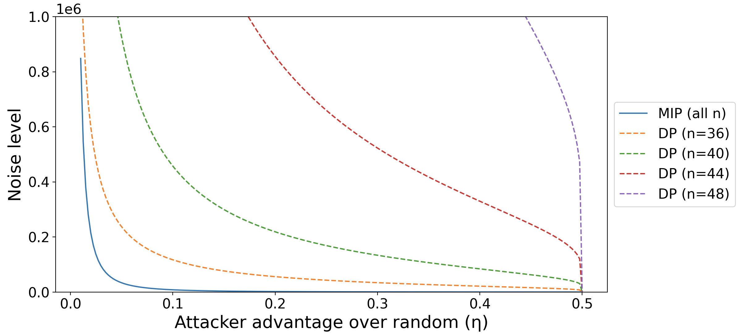
To illustrate our theoretical results, we plot the noise level needed to guarantee MIP vs. the corresponding level of DP (with the correspondence given by Theorem 4) for the example in Proposition 9.

Refer to Fig. 1. Dotted lines refer to DP, while the solid line is for MIP with $M=2$. The $x$-axis gives the best possible bound on the attacker’s improvement in accuracy over random guessing–i.e., the parameter $\eta$ for an $\eta$-MIP method–according to that method’s guarantees. For DP, the value along the $x$-axis is given by the (tight) correspondence in Theorem 4, namely $\eta=\frac{1}{1+e^{-\varepsilon}}-\frac{1}{2}$. $\eta=0$ corresponds to perfect privacy (the attacker cannot do any better than random guessing), while $\eta=\frac{1}{2}$ corresponds to no privacy (the attacker can determine membership with perfect accuracy). The $y$-axis denotes the amount of noise that must be added to the non-private algorithm’s output, as measured by the scale parameter of the Laplace noise that must be added (lower is better). For MIP, by Theorem 7, this is $(6.16/\eta)^{2}\sigma$ where $\sigma$ is an upper bound on the variance of the base algorithm over random subsets, and for DP this is $\frac{\Delta}{\log\frac{1+2\eta}{1-2\eta}}$. (This comes from solving $\eta=\frac{1}{1+e^{-\varepsilon}}-\frac{1}{2}$ for $\varepsilon$, then using the fact that $\mathrm{Laplace}(\Delta/\varepsilon)$ noise must be added to guarantee $\varepsilon$-DP.) For DP, the amount of noise necessary changes with the size $n$ of the private dataset. For MIP, the amount of noise does not change, so there is only one line.

The results show that for even small datasets ($n\geq 36$) and for $\eta\geq 0.01$, direct noise accounting for MIP gives a large advantage over guaranteeing MIP via DP. In practice, such small datasets are uncommon. As $n$ increases above even this modest range, the advantage in terms of noise reduction for MIP vs. DP quickly becomes many orders of magnitude and is not visible on the plot. (Refer to Proposition 9. The noise required for DP grows exponentially in $n$, while it remains constant in $n$ for MIP.)

We conduct an experiment as a representation scenario for private synthetic data generation. We are given a dataset which consists of i.i.d. draws from a private ground truth distribution $P$. Our goal is to learn a generative model $G$ which allows us to (approximately) sample from $P$. That is, given a latent random variable $z$ (we will take $z\sim\mathcal{N}(0,I)$), we have $G(z)\sim P$. If $G$ is itself private and a good approximation for $P$, then by the post-processing theorem (Theorem 3), we can use $G$ to generate synthetic draws from $P$, without violating the privacy of any sample in the training data.

For this experiment, we will take $G$ to be a single-layer linear network with no bias, i.e. $G(z)=Wz$ for some weight matrix $W$. The ground truth distribution $P=\mathcal{N}(0,\Sigma)$ is a mean-0 normal distribution with (unknown) non-identity covariance $\Sigma$. In this setting, $W=\Sigma^{1/2}$ would exactly reproduce $P$.

Let $\{\mathbf{x}_{i}\}_{i=1}^{n}\subseteq\mathbb{R}^{d}$ be the training data. Rather than attempting to learn $W\approx\Sigma^{1/2}$ directly, we will instead try to learn $A\approx\Sigma$. We can then set $W=(A+A^{\top})^{1/2}$. If $A\approx\Sigma$, then we will have $W\approx\Sigma^{1/2}$ and $G(z)\approx P$. We learn $A$ by minimizing the objective

via gradient descent.

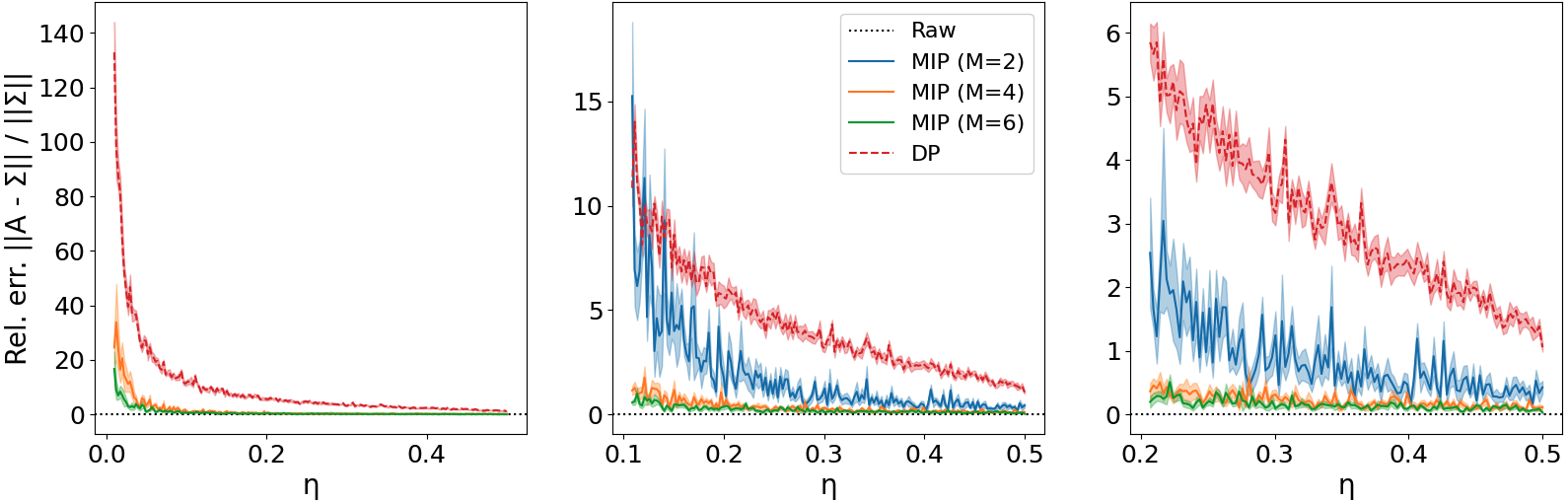
For the DP method, we implement DP-SGD (Abadi et al., 2016) with a full batch. We chose the clipping parameter $C$ according to the authors’ recommendations, i.e. the median of the unclipped gradients over the training procedure. To implement MIP, we used Corollary 8 with $M\in\{2,4,6\}$ and the corresponding $\sigma_{i}$’s computed empirically over 128 random train/holdout splits of the base dataset. The results below use $d=3$ and $n=500,000$.

Refer to Figure 2. The $x$-axes show the theoretical privacy level $\eta$ (again using the tight correspondence between $\varepsilon$ and $\eta$ from Theorem 4), and the $y$-axes show the relative error $\|A-\Sigma\|_{F}/\|\Sigma\|_{F}$ (lower is better). The three plots show the same results zoomed in on different ranges for $\eta$ to see greater granularity, and the shaded region shows the standard error of the mean over 10 runs. For $\eta\geq 0.1$, MIP with any of the tested values of $M$ outperforms DP in terms of accuracy. For the entire tested $\eta$ range (the smallest of which was $\eta=0.01$), MIP with $M=4$ or $6$ outperforms DP. (The first plot does not show MIP with $M=2$ because its error is very large when $\eta<0.1$.) Finally, observe that DP is never able to obtain relative error less than $1$ (meaning the resulting output is mostly noise), while MIP obtains relative error less than $1$ for $\eta\approx 0.2$ and larger.

References

- Abadi et al. (2016) Martin Abadi, Andy Chu, Ian Goodfellow, H Brendan McMahan, Ilya Mironov, Kunal Talwar, and Li Zhang. Deep learning with differential privacy. In Proceedings of the 2016 ACM SIGSAC conference on computer and communications security, pages 308–318, 2016.
- Assefa et al. (2020) Samuel A Assefa, Danial Dervovic, Mahmoud Mahfouz, Robert E Tillman, Prashant Reddy, and Manuela Veloso. Generating synthetic data in finance: opportunities, challenges and pitfalls. In Proceedings of the First ACM International Conference on AI in Finance, pages 1–8, 2020.
- Baluta et al. (2022) Teodora Baluta, Shiqi Shen, S Hitarth, Shruti Tople, and Prateek Saxena. Membership inference attacks and generalization: A causal perspective. ACM SIGSAC Conference on Computer and Communications Security, 2022.
- Bun et al. (2021) Mark Bun, Damien Desfontaines, Cynthia Dwork, Moni Naor, Kobbi Nissim, Aaron Roth, Adam Smith, Thomas Steinke, Jonathan Ullman, and Salil Vadhan. Statistical inference is not a privacy violation. DifferentialPrivacy.org, 06 2021. https://differentialprivacy.org/inference-is-not-a-privacy-violation/.
- Carlini et al. (2021a) Nicholas Carlini, Steve Chien, Milad Nasr, Shuang Song, Andreas Terzis, and Florian Tramer. Membership inference attacks from first principles. arXiv preprint arXiv:2112.03570, 2021a.
- Carlini et al. (2021b) Nicholas Carlini, Florian Tramer, Eric Wallace, Matthew Jagielski, Ariel Herbert-Voss, Katherine Lee, Adam Roberts, Tom Brown, Dawn Song, Ulfar Erlingsson, et al. Extracting training data from large language models. In 30th USENIX Security Symposium (USENIX Security 21), pages 2633–2650, 2021b.
- Chen et al. (2020) Dingfan Chen, Ning Yu, Yang Zhang, and Mario Fritz. Gan-leaks: A taxonomy of membership inference attacks against generative models. In Proceedings of the 2020 ACM SIGSAC conference on computer and communications security, pages 343–362, 2020.
- Dwork and Rothblum (2016) Cynthia Dwork and Guy N Rothblum. Concentrated differential privacy. arXiv preprint arXiv:1603.01887, 2016.
- Dwork et al. (2014) Cynthia Dwork, Aaron Roth, et al. The algorithmic foundations of differential privacy. Foundations and Trends® in Theoretical Computer Science, 9(3–4):211–407, 2014.
- Gerlovina and Hubbard (2019) Inna Gerlovina and Alan E Hubbard. Computer algebra and algorithms for unbiased moment estimation of arbitrary order. Cogent mathematics & statistics, 6(1):1701917, 2019.
- Gilbert and McMillan (2018) Anna C Gilbert and Audra McMillan. Property testing for differential privacy. In 2018 56th Annual Allerton Conference on Communication, Control, and Computing (Allerton), pages 249–258. IEEE, 2018.
- He et al. (2022) Xinlei He, Zheng Li, Weilin Xu, Cory Cornelius, and Yang Zhang. Membership-doctor: Comprehensive assessment of membership inference against machine learning models. arXiv preprint arXiv:2208.10445, 2022.
- Hu et al. (2022) Pingyi Hu, Zihan Wang, Ruoxi Sun, Hu Wang, and Minhui Xue. M^ 4i: Multi-modal models membership inference. Advances in Neural Information Processing Systems, 2022.
- Jagielski et al. (2020) Matthew Jagielski, Jonathan Ullman, and Alina Oprea. Auditing differentially private machine learning: How private is private sgd? Advances in Neural Information Processing Systems, 33:22205–22216, 2020.
- Jayaraman and Evans (2019) Bargav Jayaraman and David Evans. Evaluating differentially private machine learning in practice. In 28th USENIX Security Symposium (USENIX Security 19), pages 1895–1912, 2019.
- Jayaraman and Evans (2022) Bargav Jayaraman and David Evans. Are attribute inference attacks just imputation? ACM SIGSAC Conference on Computer and Communications Security, 2022.
- Jordon et al. (2022) James Jordon, Lukasz Szpruch, Florimond Houssiau, Mirko Bottarelli, Giovanni Cherubin, Carsten Maple, Samuel N Cohen, and Adrian Weller. Synthetic data–what, why and how? arXiv preprint arXiv:2205.03257, 2022.
- Kairouz et al. (2015) Peter Kairouz, Sewoong Oh, and Pramod Viswanath. The composition theorem for differential privacy. In International conference on machine learning, pages 1376–1385. PMLR, 2015.
- Liu et al. (2022) Yiyong Liu, Zhengyu Zhao, Michael Backes, and Yang Zhang. Membership inference attacks by exploiting loss trajectory. ACM SIGSAC Conference on Computer and Communications Security, 2022.
- Mironov (2017) Ilya Mironov. Rényi differential privacy. In 2017 IEEE 30th computer security foundations symposium (CSF), pages 263–275. IEEE, 2017.
- Nasr et al. (2021) Milad Nasr, Shuang Songi, Abhradeep Thakurta, Nicolas Papernot, and Nicholas Carlin. Adversary instantiation: Lower bounds for differentially private machine learning. In 2021 IEEE Symposium on security and privacy (SP), pages 866–882. IEEE, 2021.
- Office for Civil Rights (2002) HHS Office for Civil Rights. Standards for privacy of individually identifiable health information. final rule. Federal register, 67(157):53181–53273, 2002.
- Shokri et al. (2017) Reza Shokri, Marco Stronati, Congzheng Song, and Vitaly Shmatikov. Membership inference attacks against machine learning models. In 2017 IEEE symposium on security and privacy (SP), pages 3–18. IEEE, 2017.
- Stadler et al. (2022) Theresa Stadler, Bristen Oprisanu, and Carmela Troncoso. Synthetic data – anonymisation groundhog day. In 31st USENIX Security Symposium (USENIX Security 22). USENIX Association, 2022.
- Tao et al. (2021) Yuchao Tao, Ryan McKenna, Michael Hay, Ashwin Machanavajjhala, and Gerome Miklau. Benchmarking differentially private synthetic data generation algorithms. arXiv preprint arXiv:2112.09238, 2021.
- Thudi et al. (2022) Anvith Thudi, Ilia Shumailov, Franziska Boenisch, and Nicolas Papernot. Bounding membership inference. arXiv preprint arXiv:2202.12232, 2022.
- Wasserman and Zhou (2010) Larry Wasserman and Shuheng Zhou. A statistical framework for differential privacy. Journal of the American Statistical Association, 105(489):375–389, 2010.
Appendix A Deferred Proofs
For the reader’s convenience, we restate all lemmas, theorems, etc. here. See 2
Proof.
We will show that the membership inference algorithm is optimal, then compute the resulting probability of membership inference. We have
The choice of algorithm just specifies the value of for each sample and each . We see that the maximum membership inference probability is obtained when