Pseudo-Triangle Visibility Graph: Characterization and Reconstruction
Abstract
The visibility graph of a simple polygon represents visibility relations between its vertices. Knowing the correct order of the vertices around the boundary of a polygon and its visibility graph, it is an open problem to locate the vertices in a plane in such a way that it will be consistent with this visibility graph. This problem has been solved for special cases when we know that the target polygon is a tower or a spiral. Knowing that a given visibility graph belongs to a simple polygon with at most three concave chains on its boundary, a pseuodo-triangle, we propose a linear time algorithm for reconstructing one of its corresponding polygons. Moreover, we introduce a set of necessary and sufficient properties for characterizing visibility graphs of pseudo-triangles and propose polynomial algorithms for checking these properties.
keywords:
Computational geometry; Visibility graph; Characterizing visibility graph; Polygon reconstruction; Pseudo-triangle.1 Introduction
The visibility graph of a simple polygon is a graph where is the vertices of and an edge exists in if and only if the line segment lies completely inside , i.e they are visible from each other. Based on this definition, each pair of adjacent vertices on the boundary of the polygon are assumed to be visible from each other. This implies that we have always a Hamiltonian cycle in a visibility graph which determines the order of vertices on the boundary of the corresponding polygon.
Computing the visibility graph of a given simple polygon has many applications in computer graphics, computational geometry and robotics. There are several efficient polynomial time algorithms for this problem. Asano et al. [1] and Welzl [2] proposed time algorithms for computing the visibility graph of a simple polygon of vertices. This was then improved to by Hershberger[3] where is the number of edges in the visibility graph. The term is due to the time required for triangulating a simple polygon. Using the time triangulation algorithm of Chazelle [4] reduces the time complexity of Hershberger’s result to which is optimal.
This concept has been studied in reverse as well: Characterizing a visibility graph problem is to determine whether a give graph is isomorphic to the visibility graph of some simple polygon, and the reconstruction problem is to build such a simple polygon. Everett showed that these probleme are in PSPACE[5], and this is the only result known about the complexity of these problems. These problems have been solved only for special cases of spiral and tower polygons. These results are obtained by Everett and Corneil [6] for spiral polygons and by Colley et al. [7] for tower polygons. In spiral polygons there is at most one concave chain (Fig. 1a) and the boundary of a tower polygon is composed of two concave chains and a single edge (Fig. 1b).
Although there is a bit progress on this type of reconstruction problem, there have been plenty of studies on characterizing visibility graphs [8, 7, 9, 10, 6, 11]. In 1988, Ghosh introduced three necessary conditions for visibility graphs and conjectured their sufficiency[11]. In 1990, Everett proposed a counter-example graph disproving Ghosh’s conjecture[5]. She also refined Ghosh’s third necessary condition to a new stronger condition[12]. In 1992, Abello et al. built a graph satisfying Ghosh’s conditions and the stronger version of the third condition which was not the visibility graph of any simple polygon, disproving the sufficiency of these conditions[13]. In 1997, Ghosh added his fourth necessary condition and conjectured that this condition along with his first two conditions and the stronger version of the third condition are sufficient for a graph to be a visibility graph. This was also disproved by a counter-example from Streinu in 2005[14].
There are also several results about other versions of the visibility graph like point visibility graph[15, 16, 17], pseudo-polygon visibility[18, 19, 20, 21] and terrain visibility[22]. Excellent surveys on visibility graph results can be found in [23, 24, 25].

In this paper, we solve the reconstruction problem for pseudo-triangles. A pseudo-triangle is a simple polygon whose boundary is composed of three concave chains, called side-chains, where each pair shares one convex vertex (called a corner). Let be a pseudo-triangle formed by the concave side-chains , , and where , , and are the corners (Fig. 1c). According to this notation, a concave side-chain joining corner vertices and is denoted by where and are in .
Let be the Hamiltonian cycle of the visibility graph of which indicates the order of vertices on the boundary of . Here, we use the same notation for a vertex on the boundary of and its corresponding vertex in the visibility graph and . For a given pair of Hamiltonian cycle and visibility graph , we introduce a set of necessary properties on and when this pair belongs to a pseudo-triangle and prove that these properties are sufficient as well.
Having these properties, we propose a linear-time algorithm for reconstructing a pseudo-triangle with as its visibility graph. Moreover, we propose algorithms for verifying the properties on a given pair of and . These characterizing algorithms run in linear time in terms of the size of . Therefore, in this paper we solve the characterizing and reconstructing problems for another class of polygons called pseudo-triangles.
Since a tower polygon is a special case of a pseudo-triangle, we use the tower reconstruction algorithm [7] as a sub-routine in our algorithm to build the initial part of the polygon.
Our motivation in solving this problem for pseudo-triangles is that every polygon can be partitioned into pseudo-triangles. Then, an idea for solving a general reconstruction problem is to handle these steps:
-
•
Recognize a pseudo-triangle decomposition for the target polygon from and .
-
•
Reconstruct each pseudo-triangle separately.
-
•
Attach the reconstructed pseudo-triangles satisfying the pseudo-triangle decomposition and the visibility constraints.
In Section 2, we briefly describe the tower reconstruction algorithm [7] for reconstructing tower polygons which is used as a sub-routine in our algorithm. In Section 3, we introduce a set of necessary conditions(properties) of the visibility graph of pseudo-triangles and in Section 4, we prove sufficiency of these conditions by proposing a reconstruction algorithm. Finally, we analyze the running time of the reconstruction algorithm and the algorithms required to check the properties.
2 Reconstructing Tower Polygons
A strong ordering on a bipartite graph with partitions and is a pair, and , of orderings on respectively (resp.) and such that if , , and there are edges and in , the edges and also exist in .
The following theorem by Colley et al. [7] indicates the main property of the visibility graph of a tower polygon and guarantees the existence of a tower polygon consistent with such a visibility graph.
Theorem 2.1.
[7] Removing the edges of the reflex chains from the visibility graph of a tower gives an isolated vertex plus a connected bipartite graph for which the ordering of the vertices in the partitions provides a strong ordering. Conversely, any connected bipartite graph with strong ordering belongs to a tower polygon. Furthermore, such a tower can be constructed in linear time in terms of the number of vertices.

The outline of the reconstruction algorithm proposed by Colley et al. [7] is as follows. As input, it takes the corner vertex and a connected bipartite graph with vertices partitioned into two independent sets and having strong ordering.
In the first step, the position of the corner and the vertices and are determined as in Fig. 2. In a middle step, suppose that the positions of the vertices and have been determined and the directions of the half-lines from and which respectively contain and , where , are also known. To complete such a middle step, position of and the half-line from which contains (where is visible from ) must be determined. For this purpose, is located somewhere on its containing half-line horizontally below the vertex which has the minimum index among vertices of which are visible from . Then, the containing half-line of will be the half-line on the supporting line of and downward from . Here, is a point on with an distance below , when lies on . If does not lie on , then is a point on with an distance below .
According to this construction, will be the intersection of chain and the supporting line of and . Similarly, will be the intersection of and the supporting line of and (Fig. 2). We say “will” because we first fix position of (resp. ) from which position of vertex (resp. ) is determined. We will use this notation once again in Section 4.
3 Properties of Pseudo-Triangle Visibility Graphs
In this section, we describe a set of properties that a pair of and must have to be the Hamiltonian cycle and visibility graph of a pseudo-triangle.
Any sub-sequence on the Hamiltonian cycle is called a chain and is denoted by . A vertex on a chain is a blocking vertex for the invisible pair if there is no visible pair of vertices in and in . Ghosh showed that for every invisible pair of vertices in a visibility graph, there is at least one blocking vertex in or . Furthermore, every vertex on the shortest Euclidean path between and (inside the corresponding polygon) is a blocking vertex for this pair [11]. Note that in a pseudo-triangle the shortest Euclidean path between two invisible vertices turns in only one direction (i.e. clockwise or counterclockwise).
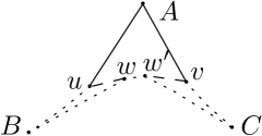
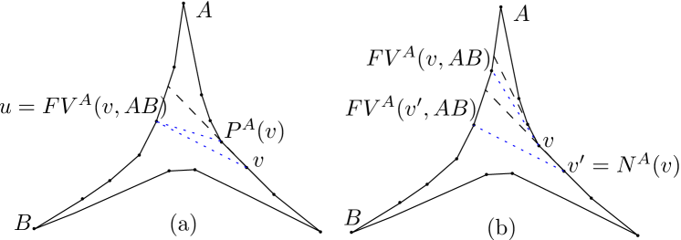
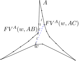
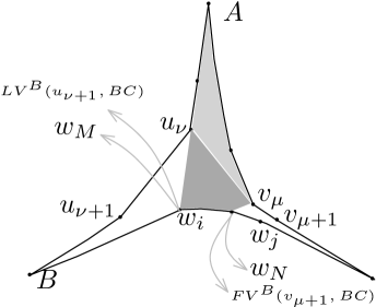
Let , , and be the side-chains of a pseudo-triangle. The order of vertices in these chains is defined with respect to one of their corner vertices. For a vertex in chain , is equal to the number of vertices in chain minus one. According to this definition, is zero and is where is the number of vertices in chain . Then, based on a given vertex indexing we refer to the previous and next vertices of a given vertex on a side-chain. For a vertex in chain with , we use to refer to the vertex with . Similarly, is the vertex with . For the sake of brevity, we use instead of , and instead of . Note that in this notation, can be a positive or negative natural number. For corner vertices which belong to two side-chains we use or notation only when the target chain is known from the context. For a vertex , is a vertex on chain with minimum index that is visible from when the indices start from corner vertex . Similarly, is a vertex on chain with maximum index that is visible from when the indices start from corner vertex . We have used and respectively as abbreviation for first visible and last visible. Fig. 3 depicts this notation.

Lemma 3.1.
It is always possible to identify at least two corners of a pseudo-triangle from its corresponding Hamiltonian cycle and visibility graph.
Proof 3.2.
Since a corner is a convex vertex, it cannot be a blocking vertex for its neighbors. Therefore, in the Hamiltonian cycle of a pseudo-triangle, there are at most three vertices whose adjacent vertices are visible pairs. By traversing the Hamiltonian cycle, these visible pairs, and the corresponding corners, can be identified.
Suppose that this method does not identify all three corners. Without loss of generality, assume that is an unidentified corner and its adjacent vertices on chains and are respectively and . This means that and do not see each other and there must be a blocking vertex for this invisible pair. Due to their concavity, this blocking vertex cannot belong to the chains and . Consider the shortest Euclidean path between and inside the pseudo-triangle(Fig. 4). It is clear that this path is composed of a subchain of , say , and two edges and where and both edges and belong to the visibility graph. The polygon formed by is a tower polygon with base and corner . The corner of this tower is the isolated vertex obtained by removing the edges of its Hamiltonian cycle from its visibility graph. Therefore, the corner vertex is detectable. The same argument holds for the tower polygon formed by from which the corner can be identified. This means that if cannot be identified from the visibility graph, the other two corners will be detectable. ∎
Consider a pseudo-triangle with side-chains , , and , and and as its visibility graph and Hamiltonian cycle, respectively. Assume that the method described in Lemma 3.1, identifies only two corners of . Without loss of generality, assume that is the unidentified vertex. This means that there is a subchain on which blocks the visibility of adjacent vertices of on chains and . Then, there is no visibility edge between a vertex from and a vertex of . By removing the edges of the Hamiltonian cycle from the visibility graph, two isolated vertices and and a connected bipartite graph, with parts and , is obtained where consists of vertices of chains and except the isolated vertices and and consists of vertices of except and . By adding the isolated vertex to , and the boundary edge to this bipartite graph that connects to its adjacent vertex on , we will have a single isolated vertex and a bipartite graph with strong ordering. Then, according to Theorem 2.1 this bipartite graph corresponds to a tower polygon with base edge and and as its visibility graph and Hamiltonian cycle, respectively. Fig. 5 shows how such a pseudo-triangle can be interpreted as a tower polygon.

Therefore, we have the following property about the pair of and of a pseudo-triangle.
Property 1
If and are respectively the Hamiltonian cycle and visibility graph of a pseudo-triangle , at least two corners of can be identified. Furthermore, if only two corners are detectable, the given and belong to a pseudo-triangle if and only if there is a tower polygon with and as its Hamiltonian cycle and visibility graph, respectively.
From this property, we assume for the remainder of this section that the method described in the proof of Lemma 3.1 identifies all three corners. Because otherwise, we can use the tower polygon algorithm to decide whether the given pair of and belong to a tower polygon( which is a special case pseudo-triangle) and obtain the answer.
An interval of a chain with endpoints and is the set of points on this chain connecting to . Note that in this definition, the endpoints of an interval are not necessarily vertices of the chain. For example, for points on edge and on edge of a chain where , the interval defined by and is the chain .
Property 2
Every non-corner vertex of a side-chain sees a single nonempty interval from anyone of the other side-chains.
Proof 3.3.
The inner angle of such a vertex is more than and its inner visibility region cannot be bounded by a single concave chain. Therefore, it will see some parts from any of the other side-chains. The continuity of these visible parts on each side-chain is proved by contradiction. Assume that a vertex sees two disjoint intervals and from meaning that the interval is not visible from . Consider an invisible point in . There must be a blocking vertex for the invisible pair . This blocking vertex must lie on the third side-chain which will also blocks either the visibility of and or and . ∎
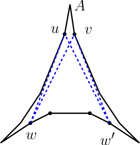
Property 3
(Fig. 6(a)) For any pair of side-chains and and a pair of vertices where , , , and , we have . In other words, the closest vertex to on which is visible to a vertex , for , is also visible from .
Proof 3.4.
Consider the subpolygon . If we triangulate this polygon, there is no internal diagonal connected to which means that must be a triangle in any triangulation. Therefore, the edge is a diagonal and this edge must exist in the visibility graph. ∎
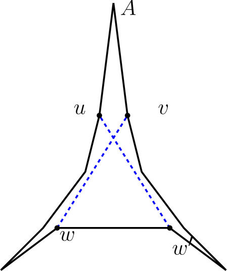
Corollary 3.5.
(Fig. 6(b)) For any pair of side-chains and and a vertex where , if and , then
.
Corollary 3.6.
For any pair of side-chains and and a vertex where , if does not see any vertex from , then does not see any vertex of as well.
Corollary 3.7.
(Fig. 7(a)) For any pair of side-chains and and a pair of vertices where and and , if both and exist in , then .
Proof 3.8.
Corollary 3.9.
(Fig. 7(b)) For any pair of side-chains and and a pair of vertices where and , if both and exist in where , then at least one of the edges or exists in .
Proof 3.10.
We prove this by induction on . For the induction base step, assume that . If is not visible from , must be equal to . Then, Property 3 implies that sees .
For the inductive step, assume that the corollary holds for all where . Lets denote and by and , respectively. If , sees both vertices and which according to Property 2 sees as well. Otherwise, according to Property 3, is visible from . If , then sees and which is farther from than and means that and see each other. Finally, when we obtain a smaller version of the problem with parameters and which holds by induction.∎
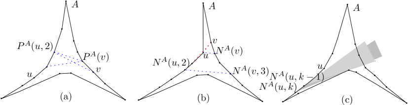
Corollary 3.11.
(Fig. 7(c)) For any pair of side-chains and and a pair of vertices and , where and none of the edges and exist in , all visible vertices of from are also visible from (for any ). This implies that must lie above .
Proof 3.12.
Any visible vertex must belong to . Otherwise, according to Corollary 3.9 either or must exist. According to Corollary 3.5, is closer to than , and because of the continuity of the chain that is visible from (Property 2) , will be visible from . This implies that is visible from all vertices of the chain . ∎
For each pair of vertices and , the diagonal edge in the visibility graph of a pseudo-triangle specifies a tower formed by the boundary vertices . The vertices of this tower satisfy the strong ordering defined earlier. This strong ordering can be derived from Property 2 and corollaries 3.7 and 3.9. Therefore, we do not specify this as a new property.
Property 4
For any pair of side-chains and and a pair of vertices and , where and none of the edges and exist in ,
Proof 3.13.
(a) Triangulating using the edge , the adjacent triangle of this edge in the opposite side of must have its third vertex on . This is due to the invisibility of and pairs. Therefore, this chain contains at least one vertex. From Property 2 we know that the visible part of from any one of vertices and is continuous and the intersection of these parts will be continuous as well.
(b) From (a) we know that the subchain is nonempty. For the sake of a contradiction, assume that is farther from than . Then, the segments and intersect each other inside the pseudo-triangle. Let be this intersection point. The subpolygon formed by the boundary vertices must be a convex polygon which completely lies inside the pseudo-triangle. Otherwise, will prevent and from seeing each other. So, the diagonal edge must exist in which is a contradiction.
(c) Let be and be . For the sake of contradiction, assume that is closer to than . Then, the edges and intersect within the pseudo-triangle. Let be this intersection point. The subpolygon formed by the boundary vertices must be a convex polygon which completely lies inside the pseudo-triangle. Otherwise, will prevent and from seeing each other. So, all diagonal edges , , and must exist in which is a contradiction. ∎
Corollary 3.14.
For any side-chain , there exists at least one vertex that sees some vertices from both of the other side-chains. Furthermore, every vertex where , sees at least one vertex from .
Proof 3.15.
If there is a pair of vertices and satisfying Property 4(a), the first part holds for the vertices of the subchain of the third side-chain which is visible from both and . If there is no such a pair of vertices, without loss of generality assume that sees some vertices of and . Trivially, the adjacent vertex of on side-chain sees both and . This can be obtained directly from Property 4(a) by imaginary cloning as two separate vertices on and . and adding new corner vertex as a point on the supporting line of and in the opposite side of .
Having a vertex satisfying the first part, the second part follows from Property 3. ∎
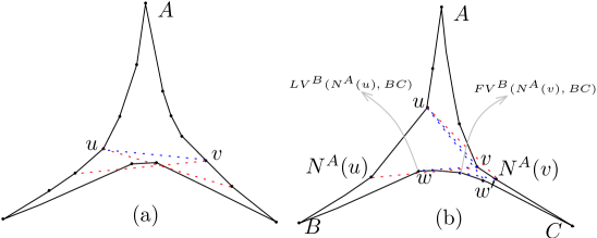
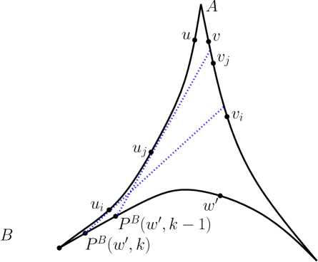
Property 5
(Fig. 9) For any side-chain and a vertex with distinct vertices and , the vertices and are visible from each other.
Proof 3.16.
Let be the subpolygon with as its boundary vertices. The vertex does not see any other vertex of which means that the diagonal must be used to triangulate . This means that and must be visible from each other. ∎
Property 6
(Fig. 10) For any side-chain , let and be respectively the closest vertices on and to which are visible from some vertex (not necessarily the same) of . Then, there exists a nonempty subchain in , and , that either all vertices of this subchain are visible from both and , or, is an edge of and sees and sees .
Proof 3.17.
It is simple to show that . Assume that there is no vertex on that sees both vertices and . Then, we first show that there is a pair of vertices and where sees and sees . Let be and be . Trivially, and is closer to than (otherwise, and will be visible to both and ). To complete the proof, it is enough to show that . This is done by showing that any vertex between and on must see at least one of the vertices and which contradicts the definition of and .
Assume that there is a vertex between and and it sees neither nor . In the tower polygon formed by boundary , the blocking vertex for the invisible pair must lie on . Similarly, in the tower formed by boundary , the blocking vertex for the invisible pair must lie on . Therefore, at least one of the side-chains and must be convex which is a contradiction. So, must see at least one of the vertices and . ∎
 |
 |
Corollary 3.18.
Proof 3.19.
For the sake of contradiction, assume that is closer to than . The diagonal edge along with vertices form a tower polygon which contains the vertices and , and satisfies strong ordering. When both edges and exist in the visibility graph, the edge must also exist in .
Property 7
Let be the subchain of satisfying Property 6 and for any vertex , and are the closest vertices to which are visible to . Then:
-
a
If , then at least one of the pairs and
are invisible. -
b
If and are invisible vertices, then this happens for all vertices in and is not farther from than . This is symmetrically true when and are invisible vertices.
-
c
If is closer to than , then is an invisible pair. Symmetrically, are invisible vertices when is closer to than .
Proof 3.20.
(a) Consider the subpolygon with boundary . The pairs and are invisible. These pairs share the same blocking vertex. If is the blocking vertex, then is an invisible pair, and if is the blocking vertex, then the pair is invisible.
(b) Assume that are invisible from each other. This means that the visible vertices of from is bounded from above by vertices of . This will happen for all vertices in as well. A similar argument holds when is the invisible pair.
(c) It is clear that at least one of the vertices and is farther from than and . For the sake of a contradiction, assume that is a visible pair. Then, in subpolygon , must be the blocking vertex for the pairs and . This vertex also blocks the pairs and . But, for some and and , , , and which contradicts the definition of . ∎
As mentioned earlier, Ghosh introduced four necessary conditions for a visibility graph of a simple polygon. It is simple to show that these conditions are derived from the properties described in this section which meas that these properties includes Ghosh’s conditions.
4 Pseudo-Triangle Reconstruction
In this section, denotes the visibility graph of a pseudo-triangle with , , and side-chains and the order of vertices on the boundary of is specified by a Hamiltonian cycle in . We assume that the inputs and satisfy the properties 1 to 7. We propose an algorithm for reconstructing a pseudo-triangle corresponding to the given pair of and .
In order to reconstruct the pseudo-triangle , we divide into four subpolygons , , , and as shown in Fig. 12 and reconstruct each one separately. For the sake of brevity, on side-chain , on side-chain , and on side-chain where . We assume that and have respectively and vertices.
The subpolygon is formed by subchains and and edge where and . The vertices and are identified by walking alternatively on side-chains and from corner vertex towards and . As a step of this trace, assume that we are at vertices and and want to go one step further on . If is the last vertex on or does not see we fix as . Otherwise, we go to in this step. Walking on side-chain are done similarly. The subpolygon is a tower polygon with strong ordering in its visibility graph. Note that or exists only when the side-chain has more than one edge, otherwise, two identified adjacent corners and compose the base of a tower polygon which can be constructed by the tower reconstruction algorithm. So, we assume that has more than one edge.
The subpolygon is identified as follows: Let be the maximum subchain of visible from both and . According to Property 4(a), this chain is nonempty and continuous. Let and . From Property 4(b), and and from Property 4(c), . We define and as and , respectively. It is clear that chain contains at least one vertex. Then, is defined to be the polygon with as its boundary.
The subpolygon is formed by subchains and and edge . Similarly, subchains and and edge specify the subpolygon . It is clear that is the union of , , , and .
Our reconstruction algorithm first builds using the tower reconstruction algorithm in such a way that vertices of lie to the left of vertices of . Then, we extend this polygon to build (Section 4.1) and build and attach and parts to this polygon (Section 4.2) to complete the construction procedure.
4.1 Reconstructing
In this step, we build the subpolygon . We know the position of vertices and from the previous step, which are also on the boundary of . To locate positions of other vertices, we show that there are nonempty regions in which these vertices can be placed.
For any vertex from which and , we define a region from which each point sees all vertices in the subchains and . Therefore, can be placed in satisfying the visibility constraints between and vertices of . We use instead of whenever and indices are not important. The region is determined as follows: Since sees and , the vertices and always exist and are well-defined. If and are identical, then and the region is defined to be the part of the cone formed by the lines through and restricted to the underneath of the line through points and . Trivially, each point of sees all vertices .
Let be the ‘’ half-plane defined by the line through and where ‘’ is ‘b’ (bottom), ‘r’ (right), or ‘l’ (left). If and are distinct vertices, according to Property 7, at least one of the pairs and do not see each other. The invisible pair is determined by applying Corollary 3.18 and Property 7.
Assume that is the invisible pair. Then, is defined to be (Fig. 13). As defined in Section 2, , and are collinear. We used instead of here because at least for we do not know the position of yet.
Any one of these half-planes forces some visibility constraints for . implies that sees both and ; implies that sees all vertices ; implies that sees all vertices ; prevents from seeing vertices ; and prevents from seeing vertices . Therefore, all points in this region satisfy the visibility constraints from to vertices .
Concavity of and implies that intersections and are not empty. Therefore, will be empty only when is empty or is empty. The first case is impossible, because otherwise, must be visible from which is in contradiction with invisibility assumption of . The second case is also impossible, because then, the pair and must be invisible. But, according to Property 5, and must be visible from each other.
Therefore, the region is nonempty and some part of this intersection lies in half-plane .
According to the above discussion, is defined by and two half-planes of . The apex of is defined to be the intersection of the corresponding lines of these two half-planes which is .
The above discussions was for the assumption that is the invisible pair. The description for the cases where is the invisible pair is symmetric: is and the apex of will be .
If the apex of lies on , Property 7 implies that the apex of will lie on as well. Furthermore, Corollary 3.18 implies that is either completely coinciding or is completely on its left. Similarly, if the apex of lies on , then the apex of lies on as well, and is either coinciding or is completely on its right.
Then, we can place the vertices of on an arbitrary concave chain inside in such a way that . This placement satisfies the visibility constraints for and . However, to guarantee the reconstruction of and , we define some constraints on this concave chain which is described in the rest of this section.
Let () be the intersection of and the line through and , () be the intersection of and the line through and , () be the intersection of and the line through and , and () be the intersection of and the line through and (see Fig. 14).
Note that although we have not yet determined positions of vertices defining , , and , we determine their containing edges from the visibility information as follows: for , if sees at least one vertex from , lies on the segment connecting and and lies on the segment connecting and . On the other hand, if sees no vertex from , then for , both and lie on the segment connecting and where has the highest index among the vertices of that see at least one vertex from . Corollary 3.11 implies that all these points lie on boundary edges of , except when and is visible to both and , for which both and for lie on . The same situation happens for and when .
The containing edge of for is determined as follows: If sees at least one vertex from , then lies on the segment connecting and , otherwise, it lies on the containing edge of (Note that according to our assumption at the beginning of Section 4, and are respectively the greatest indices of vertices and on and side-chains.). Similarly, for , if sees at least one vertex from , then lies on the segment connecting and , and otherwise, it lies on the containing edge of . Property 7 implies that all these points lie on boundary edges of or edges and .
The containing edges of and are respectively called “the floating edge in ” and “the floating edge in ”. We call these edges floating because we increase their length, and reposition their underneath vertices to enforce the concavity in building and .
We define the vertices and as follows: If has two edges, then and are both equal to (the middle vertex of ), and and are also defined to be . When has more than two edges, is defined to be when the apex of does not lie on a vertex of below its floating edge. Otherwise, is defined to be where is the maximum index for which the apex of lies above the floating edge of (this apex may lie on ). If the index of is greater than , the apex of is temporarily assumed to be and is defined to lie between and . The index is defined similarly. It is clear that at least one of the equalities or holds.
We use to denote the ray from towards . In addition, denotes the ray from and parallel to (Fig. 15).
Despite our definition of the regions for all vertices , we refine this definition for (resp. ) when (resp. ) or the floating edge of (resp. ) lies under the line through and . At most one of the floating edges lies under . Because otherwise, either will see or will see which is in contradiction with the selection of and . Let be a point on when the floating edge of lies under , or be otherwise. Similarly, is defined to be either or a point on . The regions and are restricted to lie under the line through and . Moreover, we know that at most one of the indices and is not equal to its corresponding index or . Without loss of generality, assume that . Then, we additionally restrict the region as follows (this restriction is not applied when we reconstruct or ). Let be a point inside the intersection of and and with an arbitrary positive distance from . We determine on its edge and with distance above the lower endpoint of this edge where and is the number of vertices in and whose ’s and ’s lie on this edge. The region is restricted to lie under the line through and (see Fig. 16).
Let be a point on its edge and with distance below the upper endpoint of this edge where and is the number of vertices in whose ’s lie on this edge. Similarly, let be a point on its edge and with distance above the lower endpoint of this edge where and is the number of vertices in and whose ’s and ’s lie on this edge. The value of is small enough such that lies above . The points and are defined similarly.
As shown in Fig. 15, let (resp. ) be the strip defined by the supporting lines of and (resp. and ).
Lemma 4.1.
It is always possible to enlarge the floating edges of and and re-position the vertices which lie under the enlarged edges such that and are not empty and the new position of vertices of satisfy their visibility relations in the visibility graph.
Proof 4.2.
Assume that the intersection of and is empty. According to the definition of , the apex of either lies above the floating edge of or lies on . This implies that enlarging the floating edge of only affects half-plane that defines up-side of . Then, we can enlarge the floating edge of in such a way that the lower defining ray of and the upper defining half-plane of intersect inside which means that the intersection of and is not empty. Moreover, when this intersection is not empty, this extension will just increase the intersection. On the other hand, enlarging this edge changes the position of vertices of which lie under this edge. For these vertices, we have their corresponding points ’s. By enlarging the floating edge of , the new positions will be computed according to their definition (for a vertex it must lie on the supporting line of and ) to satisfy the visibility relations in the visibility graph reduced to vertices of . To complete the proof, it is simple to see that extending the floating edge of will again increase the intersection of and .
The proof for is analogously the same. ∎
After locating the position of vertices in (by possibly extending the floating edges), we place the vertices of as follows: If , then we set as and place inside the intersection of and in such a way that both and be visible to and ; neither blocks the visibility of , nor blocks the visibility of . When , and are positioned analogously. Finally, if and , we select a point from as and a point from as again in such a way that both see and . Then, we put the vertices on a slightly concave chain from to in such a way that each () lies inside and sees and .
Based on the definition of ’s regions and the specified positions of vertices inside these regions, this setting is compatible with the visibility graph restricted to the vertices of and .
4.2 Reconstructing and
In this step, we place the vertices of and to complete the reconstruction procedure. As said before, (resp. ) is a part of the target pseudo-triangle with (resp. ) boundary vertices. Here, we only describe how to build . The construction of is symmetrically the same.
Location of a vertex is determined by the intersection point of the rays and and location of a vertex is an arbitrary point on inside the region . Therefore, to construct we start from and , and in each step we determine the position of one of the vertices and go forward to the next vertex. This is done by incrementally determining direction of the rays , , and as well as regions.
Consider the edges of the pseudo-triangle on which the points , , , , and for , , and and lie. Keep an upper point and a lower point for each edge. Initialize the upper point with the upper endpoint of that edge or the latest located or on this edge. Initialize the lower point with the lower endpoint of the edge. Position of each , , , , and is determined whenever we need the rays passing through them. We place the points , , and , with distance above the current lower point of their edges and place the points and , with distance below the upper point of their edges. Whenever a new , , , , or point is located on an edge, the upper or lower point of that edge is updated properly.
More precisely, assume that we have already determined positions of vertices () as well as the vertices (). To determine position of one of the vertices and we do as follows: Let be . If , then we have already located the position of , and directions of the rays and are known. We will show in Lemma 4.3 that these rays intersect. So, is located on the intersection point of these rays (Fig. 17(a)). Otherwise, we must first determine position of which lies on and inside (Fig. 17(b)). The position of is already known and is determined according to the above paragraph. From these two points the direction of is obtained. The region is determined as follows: Suppose that and . We define as in the previous section with the exception that it may be possible that only one of the vertices and exists. By Corollary 3.14, for , always exists. If sees no vertex from , then it would see a part of the floating edge of . Hence, we consider the upper endpoint of this edge as . From properties 5 and 7 we know that is not empty and lies to the left of . Moreover, it will be shown in Lemma 4.3 that intersects . Since passes through all , passes through . Therefore, we can determine the position of .
Note that the definition of ’s and ’s enforce the concavity of the vertices on and , respectively. According to the definition of and for and and for , in both cases (locating or ), visibility of the newly located vertex is exactly the same as its visibility in the visibility graph (restricted to the vertices of , , and the constructed part of ). This means that at the end of this construction which vertices and are located the visibility graph of the constructed polygon is consistent with the input visibility graph.
Lemma 4.3.
The rays and for are convergent inside .
Proof 4.4.
Remember that is the strip defined by the supporting lines of and . By Corollaries 3.5 and 3.11, we know that lies above the strip and lies below this strip. Then, it is enough to show that for , crosses and crosses . We first prove that intersects . Let . For , it can be easily shown by induction that is located above . Moreover, it is simple to see that must lie below . Then, knowing that crosses implies that intersects as well. From the fact that lies inside , it can also be shown by induction that for lies inside which means that crosses .
To complete the proof, we prove by induction on that crosses . It is clear that is located above which means that intersects . From the previous paragraph we know that intersects . Therefore, and will intersect at a point within . Since we put at this intersection point, as the induction step, assume that lies inside where . Then, intersects . ∎
5 Analysis
In previous sections, we proved several properties on the visibility graph of a pseudo-triangle and proposed an algorithm that constructs a pseudo-triangle for a given pair of visibility graph and Hamiltonian cycle when this pair supports these properties. In this section, we analyze the time complexity of algorithms required to check these properties and the running time of the reconstruction algorithm.
To check Property 1, we need a linear time trace on vertices of according to their order in . This is done in time. If two corners are identified in this way, the existence of a tower polygon corresponding to the pair of and can also be verified in linear time [7]. Property 2 can be verified in by a simple trace of the edge list of the visibility graph. Precisely, for each vertex we maintain the minimum index, maximum index, and number of vertices of the other side-chains and which are visible from . After finishing this trace, from these triple of parameters (minimum index, maximum index, number of visible vertices) the Property 2 is checked in time. In order to verify the rest of the properties, it is required to know the visible subchains from each vertex. These subchains are obtained as by-products using the method proposed for checking Property 2. Having these subchains for each vertex, Property 3 can be verified in .
In Property 4, for each pair of side-chains, we must find all pairs of visible vertices such that and are invisible. Having the visible subchains for each vertex, this check is done in constant time for each edge . Therefore, all pairs of vertices satisfying assumption of this property can be obtained in . Then, for each pair the three necessary conditions are checked in constant time using the maintained visible subchains of and vertices. Checking properties 5, 6 and 7 can be done in by simple trace on the side-chains. Therefore, all properties can be verified in .
To complete the analysis, we compute the running time of the reconstruction algorithm presented in Section 4. Assume that satisfies all of the properties introduced in Section 3 and we know the visible subchains of each vertex according to their order in . The side-chains of the target pseudo-triangle are identified in linear time according to the algorithm described in the proof of Lemma 3.1. Reconstructing is done using the tower reconstruction algorithm whose running time is linear in terms of the number of edges in the visibility graph reduced to . To reconstruct , the algorithm needs to determine the floating edges of and which can be done in constant time. Computing the -type regions (for each vertex ) and determining the vertices and needs time. If the conditions of Lemma 4.1 are not satisfied, the floating edges of and must be extended which is done in : A lower bound for the increase in floating edges can be computed by using Thales’ theorem and trigonometric functions. Locating each vertex of is also done in constant time. Finally, placing each vertex of and takes constant time, as well. Therefore, the total running time of the algorithm is . We can combine all results as:
Theorem 5.1.
The visibility graph and the boundary vertices of a pseudo-triangle satisfy properties 1 to 7, and conversely, for any pair of graph and Hamiltonian cycle satisfying these properties, there is a pseudo-triangle whose visibility graph and boundary vertices are respectively isomorphic to and . Checking these properties and reconstructing such a polygon can be done in .
6 Conclusion
In this paper, we considered properties of the visibility graph of a pseudo-triangle and obtained a set of necessary and sufficient conditions that such graphs must have. Then, we propose an algorithm to reconstruct a polygon from a given visibility graph which supports these properties. This characterizing and reconstructing problem, despite its long history, is still at the start of its way to be solved for all polygons.
References
- [1] T. Asano, T. Asano, L. Guibas, J. Hershberger, H. Imai, Visibility of disjoint polygons, Algorithmica 1 (1986) 49–63.
- [2] E. Welzl, Constructing the visibility graph for -line segments in time, Information Processing Letters 20 (4) (1985) 167–171.
- [3] J. Hershberger, Finding the visibility graph of a simple polygon in time proportional to its size, in: Third Annual Symposium on Computational Geometry, 1987, pp. 11–20.
- [4] B. Chazelle, Triangulating a simple polygon in linear time, Discrete and Computational Geometry 6 (1991) 485–424.
- [5] H. Everett, Visibility graph recognition, Ph.D. thesis, University of Toronto, Department of Computer Science (1990).
- [6] H. Everett, D. G. Corneil, Recognizing visibility graphs of spiral polygons, Journal of Algorithms 11 (1) (1990) 1–26.
- [7] P. Colley, A. Lubiw, J. Spinrad, Visibility graphs of towers, Computational Geometry 7 (1997) 161–172.
- [8] J. Abello, O. Egecioglu, K. Kumar, Visibility graphs of staircase polygons and the weak Bruhat order, i: From visibility graphs to maximal chains, Discrete & Computational Geometry 14 (3) (1995) 331–358.
- [9] C. R. Coullard, A. Lubiw, Distance visibility graphs, International Journal of Computational Geometry & Applications 2 (4) (1992) 349–362.
- [10] H. ElGindy, Hierarchical decomposition of polygons with applications, Ph.D. thesis, McGill University, Department of Computer Science (1985).
- [11] S. K. Ghosh, On recognizing and characterizing visibility graphs of simple polygons, in: SWAT, 1988, pp. 96–104.
- [12] S. K. Ghosh, On recognizing and characterizing visibility graphs of simple polygons, Discrete & Computational Geometry 17 (2) (1997) 143–162.
- [13] J. Abello, H. Lin, S. Pisupati, On visibility graphs of simple polygons, Congressus Numerantium (90) (1992) 119–128.
- [14] I. Streinu, Non-stretchable pseudo-visibility graphs, Computational Geometry 31 (3) (2005) 195–206.
- [15] J. Cardinal, U. Hoffmann, Recognition and Complexity of Point Visibility Graphs, in: 31st International Symposium on Computational Geometry (SoCG 2015), Vol. 34, 2015, pp. 171–185.
- [16] S. K. Ghosh, B. Roy, Some results on point visibility graphs, in: In Algorithms and Computation (WALCOM), Vol. 8344 of Lecture Notes in Computer Science, 2014, pp. 163–175.
- [17] J. Kara, A.Por, D. Wood, On the chromatic number of the visibility graph of a set of points in the plane, Discrete & Computational Geometry 34 (3) (2005) 497–506.
- [18] M. Gibson, E. Krohn, Q. Wang, A characterization of visibility graphs for pseudo-polygons, in: In Algorithms – ESA, Vol. 9294 of Lecture Notes in Computer Science, 2015, pp. 607–618.
- [19] J. O’Rourke, I. Streinu, Vertex-edge pseudo-visibility graphs: Characterization and recognition, in: In: Symposium on Computational Geometry, 1997, pp. 119–128.
- [20] J. O’Rourke, I. Streinu, The vertex-edge visibility graph of a polygon, Computational Geometry 10 (2) (1998) 105–120.
- [21] I. Streinu, Non-stretchable pseudo-visibility graphs, Computational Geometry 31 (3) (2005) 195–206.
- [22] N. S. Bidokhti, On fully characterizing terrain visibility graphs (2012).
- [23] S. Ghosh, P. Goswami, Unsolved problems in visibility graphs of points, segments and polygons, ACM Computing Surveys (CSUR) 46 (2) (2013) 22.
- [24] S. K. Ghosh, Visibility algorithms in the plane, Cambridge University Press, 2007.
- [25] J. O’Rourke, Computational geometry column 18, SIGACT News 24 (1993) 20–25.