Pseudospectra of the heat operator pencil

Krishna Kumar G Department of Mathematics, University of Kerala, Kariavattom Campus, Thiruvananthapuram, Kerala, India, 695581. krishna.math@keralauniversity.ac.in and Judy Augustine Department of Mathematics, University of Kerala, Kariavattom Campus, Thiruvananthapuram, Kerala, India, 695581. judyaugustine9@gmail.com

Abstract.

This article undertakes an analysis of the one-dimensional heat equation, wherein the Dirichlet condition is applied at the left end and Neumann condition at the right end. The heat equation is restructured as a non-self-adjoint $2\times 2$ unbounded block operator matrix pencil. The spectral, pseudospectral, and $(n,\epsilon)$ -pseudospectral enclosures of the $2\times 2$ unbounded block operator matrix pencil are explored to scrutinize the heat operator pencil. The plots of the discretized equation are depicted to illustrate the observations.

Key words and phrases:

Heat equation, operator pencil, block operator matrices, non-self-adjoint, eigenvalue, pseudospectrum

2020 Mathematics Subject Classification:

Primary ; Secondary

2020 Mathematics Subject Classification:

Primary 35K05, 47A08, 47A10; Secondary 15A22, 47A30, 80M20

The first author is supported through the SERB MATRICS grant with project reference no. MTR/2021/000028 and the PLEASE scheme, Department of Higher Education, Government of Kerala, Kerala, India.

The second author thanks Kerala State Council for Science, Technology and Environment (KSCSTE), Kerala, India (Ref No: KSCSTE/990/2021-FSHP-MS) for financial support.

1. Introduction

The heat transfer through an ideal rod of length $d$ with thermal diffusivity $c^{2}$ subject to the Dirichlet condition at the left and Neumann condition at the right end is formulated as,

(1.1)

\displaystyle\frac{\partial\phi}{\partial t}=c^{2}\frac{\partial^{2}\phi}{\partial x^{2}},\ \ 0\leq x\leq d,\ \ t\geq 0,\ \ \phi(0,t)=\phi_{x}(d,t)=0.

The domain of the solution (one-dimensional heat equation) is a semi-infinite strip of width $d$ that continues indefinitely in time. The probabilistic approach, variational iteration, finite difference, and finite element are among the few methods used to study the one-dimensional heat equation; see [2, 12, 16, 22]. The one-dimensional heat equation is reformulated in this article as a linear evolution process on a suitable Hilbert space. The closed linear operator pencil arising from the heat equation is illustrated as follows. Let $u=\begin{pmatrix}u_{1}\\ u_{2}\end{pmatrix}=\begin{pmatrix}\phi\\ \phi_{x}\end{pmatrix}$ , then the system (1.1) is converted into

(1.2)

\displaystyle\mathcal{B}u_{t}=\mathcal{A}u,\ \ \mathcal{A}=\begin{pmatrix}c^{2}\cfrac{\partial^{2}}{\partial x^{2}}&&\\ &&\end{pmatrix},\ \ \mathcal{B}=\begin{pmatrix}I&\\ \cfrac{\partial}{\partial x}&-I\end{pmatrix},\ \ u_{1}(0,t)=u_{2}(d,t)=0.

Suppose $u$ is variably separable and let

u(x,t)=e^{\lambda t}\psi(x)=e^{\lambda t}\begin{pmatrix}\psi_{1}(x)\\ \psi_{2}(x)\end{pmatrix}.

Then the system (1.2) is converted into the generalized eigenvalue problem of the form

(1.3)

\displaystyle(\lambda B-A)\psi=0,\ \ A=\begin{pmatrix}c^{2}\cfrac{d^{2}}{dx^{2}}&&\\ &&\end{pmatrix},\ \ B=\begin{pmatrix}I&\\ \cfrac{d}{dx}&-I\end{pmatrix},\ \ \psi_{1}(0)=\psi_{2}(d)=0.

Thus, the one-dimensional heat equation defined in (1.1) is transformed into a linear operator pencil, a $2\times 2$ unbounded block operator matrix pencil. If $(\lambda B-A)\psi=0$ for some $\psi\neq 0$ , then $\lambda$ is called the generalized eigenvalue and $\psi$ is the corresponding generalized eigenfunction. The domains $D(A)$ and $D(B)$ are suitable subspaces of the Hilbert space $L^{2}[0,d]\times L^{2}[0,d]$ defined by

\displaystyle D(A)

\displaystyle=\left\{v\in L^{2}[0,d]:v^{\prime}\ \textnormal{is absolutely continous},\ v^{\prime\prime}\in L^{2}[0,d]\right\}\times L^{2}[0,d],

and

\displaystyle D(B)

\displaystyle=\left\{v\in L^{2}[0,d]:v\ \textnormal{is absolutely continous},\ v^{\prime}\in L^{2}[0,d]\right\}\times L^{2}[0,d].

Note that $B^{2}=I$ on $D(B)$ and for $\psi=\begin{pmatrix}\psi_{1}\\ \psi_{2}\end{pmatrix}\in L^{2}[0,d]\times L^{2}[0,d]$ ,

\displaystyle\|\psi\|^{2}=\int_{0}^{d}\left(\left|\psi_{1}(x)\right|^{2}+\left|\psi_{2}(x)\right|^{2}\right)\ dx.

In [11], Nagel introduces the matrix theory for unbounded operator matrices. One can find vast information about block operator matrices in [21]. This article focuses on the pseudospectral study of closed linear operator pencil and $2\times 2$ unbounded block operator matrix pencil to analyze the one-dimensional heat equation.

1.1. Background and Outline

The operators that arise from the physical applications are closed but unbounded, and due to this, closed operators gained attention in the mathematical field. For more about closed operators, refer [7, 8]. Throughout this article, $\mathbb{H}$ denotes a complex Hilbert space, and $I,{\bf 0}$ are the identity operator, zero operators on $\mathbb{H}$ . Further $\mathcal{C}(\mathbb{H}),\mathcal{B}(\mathbb{H})$ are the set of all closed, bounded operators on $\mathbb{H}$ . The domain of $A\in\mathcal{C}(\mathbb{H})$ is denoted as $D(A)$ .

Let $A,B\in\mathcal{C}(\mathbb{H})$ and $\lambda\in\mathbb{C}$ , then the closed linear operator pencil

(A,B)(\lambda)=\lambda B-A

is defined on $D(A)\cap D(B)$ . If both $A$ and $B$ are self-adjoint, then $(A,B)$ is called a self-adjoint pencil. For more information on self-adjoint operator pencils, see [10]. The generalized resolvent of $(A,B)$ is defined by

\rho(A,B)=\{\lambda\in\mathbb{C}:(\lambda B-A)^{-1}\in\mathcal{B}(\mathbb{H})\}.

The spectrum of $(A,B)$ is defined by $\sigma(A,B)=\mathbb{C}\setminus\rho(A,B)$ . The generalized eigenvalues of $(A,B)$ is defined by

\sigma_{e}(A,B)=\{\lambda\in\mathbb{C}:\lambda B-A\ \textnormal{is not one-one}\}.

The spectral analysis of operators fails to provide the correct information while dealing with non-normal operators. During the 1990s, Trefethen advocated the concept of pseudospectrum in the context of non-normal operators resulting from the discretization of certain non-symmetric differential operators; see [18, 19].

Definition 1.1.

Let $A\in\mathcal{C}(\mathbb{H})$ and $\epsilon>0$ , the $\epsilon$ -pseudospectrum of $A$ is defined by

\Lambda_{\epsilon}(A)=\sigma(A)\cup\left\{\lambda\in\mathbb{C}:\left\|(\lambda I-A)^{-1}\right\|\geq\epsilon^{-1}\right\}.

Pseudospectra has been extensively studied due to its applications in numerical analysis and differential equations. It is used to study the norm behavior of $A^{n}$ ( $n=1,2,\ldots$ ) and $e^{tA}$ ( $t>0$ ), analyze iterative methods for the solutions of $Ax=b$ , and in stability analysis of the method of lines discretizations of time-dependent partial differential equations; see [13, 18, 20]. Over the periods, pseudospectrum has been studied for various differential operators like wave, convection-diffusion, and Orr-Sommerfield operators; see [3, 14, 15]. Pseudospectra provides more stable information about non-self-adjoint operators under various limiting procedures than the spectrum; see [1]. Later on, Hansen introduced the more general $(n,\epsilon)$ -pseudospectra for linear operators on separable Hilbert spaces and pointed out that they have numerous attractive features with pseudospectra but offer a better insight into the approximation of the spectrum; see [4, 5]. The $(n,\epsilon)$ -pseudospectrum of bounded linear operator pencils is studied in [9].

The article is organized as follows. Section 1 illustrates the formulation of the one-dimensional heat equation into a closed linear operator pencil. The suitable substitution and the separation of variables transform the one-dimensional heat equation to a $2\times 2$ unbounded block operator matrix pencil. Section 2 studies the $(n,\epsilon)$ -pseudospectra of closed linear operator pencil. Several important properties of the $(n,\epsilon)$ -pseudospectrum of a closed linear operator pencil are developed. The equivalent definitions for the $(n,\epsilon)$ -pseudospectra of closed linear operator pencil and the characterization of the $(n,\epsilon)$ -pseudospectra of self-adjoint operator pencil are done. Section 3 concerns the $2\times 2$ unbounded block operator matrix pencil. Using the generalized Frobenius-Schur factorization, we furnish the spectral, pseudospectral, and $(n,\epsilon)$ -pseudospectral enclosures for $2\times 2$ unbounded block operator matrix pencil. Section 4 identifies the heat operator pencil as a non-self-adjoint pencil. The eigenvalue analysis and the pseudospectral enclosure of the heat operator pencil are done. The pseudospectrum of discretized heat equation is plotted to illustrate the results.

2. $(n,\epsilon)$ -pseudopsectra of the closed linear operator pencil

This section studies the $(n,\epsilon)$ -pseudospectrum of a closed linear operator pencil for a general purpose. Let $\mathbb{Z}_{+}$ denote the set of all positive integers. For $z\in\mathbb{C}$ and $r>0$ , $D(z,r):=\{\lambda:|\lambda-z|\leq r\}$ and $D(0,r)$ is denoted as $\Delta_{r}$ . For $\Omega\subseteq\mathbb{C}$ , $\overline{\Omega}:=\{\overline{\lambda}:\lambda\in\Omega\}$ .

Definition 2.1.

Let $A,B\in\mathcal{C}(\mathbb{H})$ , $n\in\mathbb{Z}_{+}\cup\{0\}$ , and $\epsilon>0$ . The $(n,\epsilon)$ -pseudospectrum of $(A,B)$ is denoted by $\Lambda_{n,\epsilon}(A,B)$ and is defined by

\Lambda_{n,\epsilon}(A,B)=\sigma(A,B)\cup\left\{\lambda\in\mathbb{C}:\left\|(\lambda B-A)^{-2^{n}}\right\|^{\frac{1}{2^{n}}}\geq\epsilon^{-1}\right\}.

The generalized $(n,\epsilon)$ -pseudoresolvent of $(A,B)$ is denoted by $\rho_{n,\epsilon}(A,B)$ and is defined by

\rho_{n,\epsilon}(A,B)=\rho(A,B)\cap\left\{\lambda\in\mathbb{C}:\left\|(\lambda B-A)^{-2^{n}}\right\|^{\frac{1}{2^{n}}}<\epsilon^{-1}\right\}.

The following observations about the pseudospectra of closed linear operator pencil are trivial.

Remark 2.2.

Let $A,B\in\mathcal{C}(\mathbb{H})$ , $n\in\mathbb{Z}_{+}\cup\{0\}$ , and $\epsilon>0$ . Then

(1)

$\sigma(A,B)\subseteq\Lambda_{n,\epsilon}(A,B)$ .
(2)

If $B=I$ , then $\Lambda_{n,\epsilon}(A,I)=\Lambda_{n,\epsilon}(A)$ .
(3)

If $n=0$ , then $\Lambda_{n,\epsilon}(A,B)=\Lambda_{\epsilon}(A,B)$ .

Lemma 2.3.

Let $A,B\in\mathcal{C}(\mathbb{H})$ and $\epsilon>0$ . Then $\sigma(A+C,B)\subseteq\Lambda_{\epsilon}(A,B)$ for every $C\in\mathcal{B}(\mathbb{H})$ with $\|C\|\leq\epsilon$ .

Proof.

Suppose $\lambda\in\sigma(A+C,B)$ and $\lambda\notin\sigma(A,B)$ , then

\lambda B-A-C=\left(\lambda B-A\right)\left(I-\left(\lambda B-A\right)^{-1}C\right).

It follows that

1\leq\left\|\left(\lambda B-A\right)^{-1}C\right\|\leq\left\|\left(\lambda B-A\right)^{-1}\right\|\left\|C\right\|.

Hence $\lambda\in\Lambda_{\epsilon}(A,B)$ for $\|C\|\leq\epsilon$ . ∎

Theorem 2.4.

Let $A,B\in\mathcal{C}(\mathbb{H})$ , $n\in\mathbb{Z}_{+}\cup\{0\}$ , and $\epsilon>0$ . Then the following holds.

(1)

$\Lambda_{n+1,\epsilon}(A,B)\subseteq\Lambda_{n,\epsilon}(A,B)$ .
(2)

$\Lambda_{n,\epsilon_{1}}(A,B)\subseteq\Lambda_{n,\epsilon_{2}}(A,B)$ for every $0<\epsilon_{1}\leq\epsilon_{2}$ .
(3)

$\displaystyle\sigma(A,B)=\bigcap_{\epsilon>0}\Lambda_{n,\epsilon}(A,B)$ .
(4)

$\Lambda_{n,\epsilon}(A,B)+\Delta_{\delta}\subseteq\Lambda_{\epsilon}(A,B)+\Delta_{\delta}\subseteq\Lambda_{\epsilon+\delta\|B\|}(A,B)$ for every $B\in\mathcal{B}(\mathbb{H})$ and $\delta>0$ .
(5)

$\Lambda_{n,\epsilon}(\alpha A,\alpha B)=\Lambda_{n,\frac{\epsilon}{|\alpha|}}(A,B)$ for every $\alpha\neq 0$ .
(6)

$\Lambda_{n,\epsilon}(\beta A+\alpha B,B)=\alpha+\beta\,\Lambda_{n,\frac{\epsilon}{|\beta|}}(A,B)$ for every $\alpha,\beta\in\mathbb{C}$ with $\beta\neq 0.$

Proof.

(1)

Suppose $\lambda\in\Lambda_{n+1,\epsilon}(A,B)\setminus\sigma(A,B)$ . Then

	$\displaystyle\epsilon^{-1}\leq\left\\|[(\lambda B-A)^{-1}]^{2^{n+1}}\right\\|^{\frac{1}{2^{n+1}}}$	$\displaystyle\leq\left\\|[(\lambda B-A)^{-1}]^{2^{n}}\right\\|^{\frac{1}{2^{n+1}}}\left\\|[(\lambda B-A)^{-1}]^{2^{n}}\right\\|^{\frac{1}{2^{n+1}}}$
		$\displaystyle=\left\\|[(\lambda B-A)^{-1}]^{2^{n}}\right\\|^{\frac{1}{2^{n}}}.$

Hence $\lambda\in\Lambda_{n,\epsilon}(A,B)\setminus\sigma(A,B)$ .

(2)

Let $0<\epsilon_{1}\leq\epsilon_{2}$ and $\lambda\in\Lambda_{n,\epsilon_{1}}(A,B)$ . If $\lambda\in\sigma(A,B)$ , then $\lambda\in\Lambda_{n,\epsilon_{2}}(A,B)$ . If $\lambda\in\Lambda_{n,\epsilon_{1}}(A,B)\setminus\sigma(A,B)$ , then

$\left\|(\lambda B-A)^{-2^{n}}\right\|^{\frac{1}{2^{n}}}\geq\epsilon_{1}^{-1}\geq\epsilon_{2}^{-1}.$

Hence $\lambda\in\Lambda_{n,\epsilon_{2}}(A,B)$ .
(3)

If $\lambda\in\sigma(A,B)$ , then $\lambda\in\Lambda_{n,\epsilon}(A,B)$ for every $\epsilon>0$ and $\displaystyle\lambda\in\bigcap_{\epsilon>0}\Lambda_{n,\epsilon}(A,B)$ . Next assume that $\displaystyle\lambda\in\bigcap_{\epsilon>0}\Lambda_{n,\epsilon}(A,B)$ and $\lambda\notin\sigma(A,B)$ , then

$\left\|(\lambda B-A)^{-2^{n}}\right\|^{\frac{1}{2^{n}}}\geq\epsilon^{-1}\ \ \ \ \text{for every}\ \epsilon>0.$

Hence $\left\|(\lambda B-A)^{-2^{n}}\right\|=0$ , a contradiction.

(4)

From (1), $\Lambda_{n,\epsilon}(A,B)\subseteq\Lambda_{\epsilon}(A,B)$ and hence $\Lambda_{n,\epsilon}(A,B)+\Delta_{\delta}\subseteq\Lambda_{\epsilon}(A,B)+\Delta_{\delta}$ . Let $\lambda\in\Lambda_{\epsilon}(A,B)$ , $\mu\in\mathbb{C}$ , and $|\mu|\leq\delta$ . If $\lambda\in\sigma(A,B)$ , from Lemma 2.3,

\lambda+\mu\in\sigma(A+\mu B,B)\subseteq\Lambda_{\delta\|B\|}(A,B)\subseteq\Lambda_{\epsilon+\delta\|B\|}(A,B).

If $\lambda\in\Lambda_{\epsilon}(A,B)\setminus\sigma(A,B)$ and $\lambda+\mu\in\sigma(A,B)$ , then $\lambda+\mu\in\Lambda_{\epsilon+\delta\|B\|}(A,B)$ . Further if $\lambda\in\Lambda_{\epsilon}(A,B)\setminus\sigma(A,B)$ and $(\lambda+\mu)B-A$ is invertible. Choose $x\in D(A)$ with $\|x\|=1$ such that $\|(\lambda B-A)x\|\leq\epsilon$ , then

	$\displaystyle 1=\\|x\\|$	$\displaystyle=\left\\|\left(\left(\lambda+\mu\right)B-A\right)^{-1}\left(\left(\lambda+\mu\right)B-A\right)x\right\\|$
		$\displaystyle\leq\left(\epsilon+\delta\\|B\\|\right)\left\\|\left(\left(\lambda+\mu\right)B-A\right)^{-1}\right\\|.$

Hence $\lambda+\mu\in\Lambda_{\epsilon+\delta\|B\|}(A,B)$ .

(5)

Let $\alpha\neq 0$ , then $\sigma(\alpha A,\alpha B)=\sigma(A,B)$ . Also

	$\displaystyle\lambda\in\Lambda_{n,\epsilon}(\alpha A,\alpha B)\setminus\sigma(\alpha A,\alpha B)$	$\displaystyle\Longleftrightarrow\left\\|(\lambda\alpha B-\alpha A)^{-2^{n}}\right\\|^{\frac{1}{2^{n}}}\geq\epsilon^{-1}$
		$\displaystyle\Longleftrightarrow\left\\|(\lambda B-A)^{-2^{n}}\right\\|^{\frac{1}{2^{n}}}\geq\frac{\|\alpha\|}{\epsilon}$
		$\displaystyle\Longleftrightarrow\lambda\in\Lambda_{n,\frac{\epsilon}{\|\alpha\|}}(A,B)\setminus\sigma(A,B).$

(6)

Let $\alpha,\beta\in\mathbb{C}$ and $\beta\neq 0$ , then

	$\displaystyle\rho(\beta A+\alpha B,B)$	$\displaystyle=\{\lambda\in\mathbb{C}:\left(\lambda B-\beta A-\alpha B\right)^{-1}\in\mathcal{B}(\mathbb{H})\}$
		$\displaystyle=\left\{\lambda\in\mathbb{C}:\left(\frac{\lambda-\alpha}{\beta}B-A\right)^{-1}\in\mathcal{B}(\mathbb{H})\right\}.$

i.e., $\lambda\in\sigma(\beta A+\alpha B,B)\Longleftrightarrow\frac{\lambda-\alpha}{\beta}\in\sigma(A,B)\Longleftrightarrow\lambda\in\alpha+\beta\,\sigma(A,B).$ Also

	$\displaystyle\lambda\in\Lambda_{n,\epsilon}(\beta A+\alpha B,B)\setminus\sigma(\beta A+\alpha B,B)$	$\displaystyle\Longleftrightarrow\left\\|(\lambda B-\beta A-\alpha B)^{-2^{n}}\right\\|^{\frac{1}{2^{n}}}\geq\epsilon^{-1}$
		$\displaystyle\Longleftrightarrow\ \frac{1}{\|\beta\|}\left\\|\left(\frac{\lambda-\alpha}{\beta}B-A\right)^{-2^{n}}\right\\|^{\frac{1}{2^{n}}}\geq\epsilon^{-1}$
		$\displaystyle\Longleftrightarrow\ \frac{\lambda-\alpha}{\beta}\in\Lambda_{n,\frac{\epsilon}{\|\beta\|}}(A,B)\setminus\sigma(A,B)$
		$\displaystyle\Longleftrightarrow\ \lambda\in\alpha+\beta\,\Lambda_{n,\frac{\epsilon}{\|\beta\|}}(A,B)\setminus\sigma(A,B).$

∎

The following theorem presents some equivalent definitions for $(n,\epsilon)$ -pseudospectra of closed linear operator pencil.

Theorem 2.5.

Let $A,B\in\mathcal{C}(\mathbb{H})$ , $n\in\mathbb{Z}_{+}\cup\{0\}$ , and $\epsilon>0$ . Then the following are equivalent.

(1)

$z\in\Lambda_{n,\epsilon}(A,B)$ .
(2)

$z\in\sigma(A,B)\cup\left\{\lambda\in\mathbb{C}:\,\left\|(\lambda B-A)^{2^{n}}u\right\|\leq{\epsilon}^{2^{n}},u\in D(A)\cap D(B),\|u\|=1\right\}.$
(3)

$z\in\sigma(A,B)\cup\Big{\{}\lambda\in\mathbb{C}:\left[(\lambda B-A)^{2^{n}}-E\right]u=0,\|E\|\leq{\epsilon}^{2^{n}},u\in D(A)\cap D(B),\|u\|=1\Big{\}}.$

Proof.

(1) $\Longrightarrow$ (2). If $z\in\Lambda_{n,\epsilon}(A,B)\setminus\sigma(A,B)$ , then $\left\|(zB-A)^{-2^{n}}\right\|^{\frac{1}{2^{n}}}\geq\epsilon^{-1}$ also there exists $x\in D(A)\cap D(B)$ with $\|x\|=1$ such that $\left\|(zB-A)^{-2^{n}}x\right\|^{\frac{1}{2^{n}}}\geq\epsilon^{-1}$ . Define $v=(zB-A)^{-2^{n}}x$ and $\displaystyle u=\frac{v}{\|v\|}$ . Then $v\neq 0$ and

\left\|(zB-A)^{2^{n}}\frac{v}{\|v\|}\right\|=\frac{\|x\|}{\left\|(zB-A)^{-2^{n}}x\right\|}\leq\epsilon^{2^{n}}.

(2) $\Longrightarrow$ (3). Suppose $\left\|(zB-A)^{2^{n}}u\right\|\leq{\epsilon}^{2^{n}}$ for some $u\in D(A)\cap D(B)$ with $\|u\|=1$ . Then there exists $\phi\in\mathbb{H}^{\prime}$ such that $\|\phi\|=1$ and $\phi(u)=\|u\|=1$ . Define rank one operator $E:\mathbb{H}\rightarrow\mathbb{H}$

E(x)=\phi(x)(zB-A)^{2^{n}}u.

Then $\|E\|\leq{\epsilon}^{2^{n}}$ and $\left[(zB-A)^{2^{n}}-E\right]u=0$ .
(3) $\Longrightarrow$ (1). Suppose $\left[(zB-A)^{2^{n}}-E\right]u=0$ for some $E\in\mathcal{B}(\mathbb{H})$ with $\|E\|\leq{\epsilon}^{2^{n}}$ and $u\in D(A)\cap D(B)$ with $\|u\|=1$ . For $z\notin\sigma(A,B)$ , we have $u=(zB-A)^{-2^{n}}Eu$ , also

\displaystyle 1=\|u\|=\left\|(zB-A)^{-2^{n}}Eu\right\|

\displaystyle\leq\left\|(zB-A)^{-2^{n}}\right\|{\epsilon}^{2^{n}}.

Thus $z\in\Lambda_{n,\epsilon}(A,B).$ ∎

Theorem 2.6.

Let $A,B\in\mathcal{C}(\mathbb{H})$ and $B(\lambda_{0}B-A)^{-1}$ is bounded for some $\lambda_{0}\in\rho(A,B)$ . Then

(\lambda B-A)^{-1}=(\lambda_{0}B-A)^{-1}\sum_{m=0}^{\infty}\left(\lambda-\lambda_{0}\right)^{m}\left[B(\lambda_{0}B-A)^{-1}\right]^{m},

for every $\lambda$ with $\displaystyle\left|\lambda-\lambda_{0}\right|<\frac{1}{\left\|B(\lambda_{0}B-A)^{-1}\right\|}$ .

Proof.

Let $\lambda\in\rho(A,B)$ , then

	$\displaystyle(\lambda B-A)^{-1}$	$\displaystyle=-\left[\left(A-\lambda_{0}B\right)-\left(\lambda-\lambda_{0}\right)B\right]^{-1}$
		$\displaystyle=-\left(A-\lambda_{0}B\right)^{-1}\left[I-\left(\lambda-\lambda_{0}\right)B\left(A-\lambda_{0}B\right)^{-1}\right]^{-1}$
		$\displaystyle=(\lambda_{0}B-A)^{-1}\left[I-\left(\lambda-\lambda_{0}\right)B(\lambda_{0}B-A)^{-1}\right]^{-1}.$

If $\displaystyle\left|\lambda-\lambda_{0}\right|<\frac{1}{\left\|B(\lambda_{0}B-A)^{-1}\right\|}$ , then

(\lambda B-A)^{-1}=(\lambda_{0}B-A)^{-1}\sum_{m=0}^{\infty}\left(\lambda-\lambda_{0}\right)^{m}\left[B(\lambda_{0}B-A)^{-1}\right]^{m}.

∎

Lemma 2.7.

Let $A,B\in\mathcal{C}(\mathbb{H})$ and $B(\lambda B-A)^{-1}$ is bounded for every $\lambda\in\rho(A,B)$ . Then the resolvent function of the operator pencil $(A,B)$ is analytic on $\rho(A,B)$ .

Proof.

Let $\lambda,\mu\in\rho(A,B)$ ,

(\lambda B-A)^{-1}-(\mu B-A)^{-1}=(\mu-\lambda)(\lambda B-A)^{-1}B(\mu B-A)^{-1}.

Then

\lim_{\lambda\rightarrow\mu}\frac{(\lambda B-A)^{-1}-(\mu B-A)^{-1}}{\lambda-\mu}=-(\mu B-A)^{-1}B(\mu B-A)^{-1}.

∎

Theorem 2.8.

Let $A,B\in\mathcal{C}(\mathbb{H})$ , $n\in\mathbb{Z}_{+}\cup\{0\}$ , and $\epsilon>0$ . If $B(\lambda B-A)^{-1}$ is bounded for every $\lambda\in\rho(A,B)$ , then

(i)

$\Lambda_{n,\epsilon}(A,B)$ is a closed subset of $\mathbb{C}$ .
(ii)

Any bounded component of $\Lambda_{n,\epsilon}(A,B)$ has non empty intersection with $\sigma(A,B)$ .

Proof.

(i)

From Theorem 2.6, $\sigma(A,B)$ is closed. Define $f:\rho(A,B)\rightarrow[0,\infty)$ by

f(\lambda)=\left\|(\lambda B-A)^{-2^{n}}\right\|^{\frac{1}{2^{n}}}.

Then $f$ is continuous and

\left\{\lambda\in\rho(A,B):\left\|(\lambda B-A)^{-2^{n}}\right\|^{\frac{1}{2^{n}}}\geq\epsilon^{-1}\right\}=f^{-1}\left(\left[\epsilon^{-1},\infty\right)\right),

is closed. Hence $\Lambda_{n,\epsilon}(A,B)$ is closed.

(ii)

Suppose $\Omega$ be a bounded component of $\Lambda_{n,\epsilon}(A,B)$ such that $\Omega\cap\sigma(A,B)=\emptyset$ . Then

\Omega\subseteq\rho(A,B)\cap\left\{\lambda\in\rho(A,B):\left\|(\lambda B-A)^{-2^{n}}\right\|^{\frac{1}{2^{n}}}\geq\epsilon^{-1}\right\}.

Let $G=\Omega\cap\left\{\lambda\in\rho(A,B):\left\|(\lambda B-A)^{-2^{n}}\right\|>\epsilon^{-{2^{n}}}\right\}$ . We claim that $G$ is open. Let $\mu\in G$ , since $\mu\in\left\{\lambda\in\rho(A,B):\left\|(\lambda B-A)^{-2^{n}}\right\|>\epsilon^{-{2^{n}}}\right\}$ , there exists $r_{\mu}>0$ , such that $D(\mu,r_{\mu})\subset\left\{\lambda\in\rho(A,B):\left\|(\lambda B-A)^{-2^{n}}\right\|>\epsilon^{-{2^{n}}}\right\}.$ Since $\Omega$ is component, $\mu\in\Omega$ and $D(\mu,r_{\mu})$ is connected, $D(\mu,r_{\mu})\subset\Omega.$ Hence $D(\mu,r_{\mu})\subset G$ . Now the map

\lambda\mapsto\left\|(\lambda B-A)^{-2^{n}}\right\|,

defined from $G$ to $\mathbb{C}$ is subharmonic and continuous on $\overline{G}$ . For any boundary point $\lambda\in G$ , $\left\|(\lambda B-A)^{-2^{n}}\right\|=\epsilon^{-{2^{n}}}$ . But for $\lambda\in G$ , $\left\|(\lambda B-A)^{-2^{n}}\right\|>\epsilon^{-{2^{n}}}$ . This contradicts the maximum principle.

∎

Theorem 2.9.

Let $A,B\in\mathcal{C}(\mathbb{H})$ such that $D(A),D(B),D(A+B),D(AB)$ are dense in $\mathbb{H}$ , $n\in\mathbb{Z}_{+}\cup\{0\}$ , and $\epsilon>0$ .

(i)

If $A$ or $B$ in $\mathcal{B}(\mathbb{H})$ , then $\Lambda_{\epsilon}(A^{*},B^{*})=\overline{\Lambda_{\epsilon}(A^{*},B^{*})}$ .
(ii)

If $A,B\in\mathcal{B}(\mathbb{H})$ , then $\Lambda_{n,\epsilon}(A^{*},B^{*})=\overline{\Lambda_{n,\epsilon}(A^{*},B^{*})}$ .

Proof.

(i)

Let $A$ or $B$ in $\mathcal{B}(\mathbb{H})$ , then $A^{*}+B^{*}=\left(A+B\right)^{*}$ ; see [17]. If $\lambda\in\sigma(A,B)$ then $\overline{\lambda}\in\sigma(A^{*},B^{*})$ . Further if $\lambda\in\Lambda_{\epsilon}(A,B)\setminus\sigma(A,B)$ , then

$\left\|(\lambda B-A)^{-1}\right\|=\left\|\left(\ \overline{\lambda}B^{*}-A^{*}\right)^{-1}\right\|\geq\epsilon^{-1}.$

The latest step follows as $(\lambda B-A)^{-1}\in\mathcal{B}(\mathbb{H})$ ; see [18]. Hence $\Lambda_{\epsilon}(A,B)\subseteq\overline{\Lambda_{\epsilon}(A^{*},B^{*})}$ . Since $D(A),D(B)$ are dense in $\mathbb{H}$ , the other inclusion follows.

(ii)

Let $A\in\mathcal{B}(\mathbb{H})$ , then $(A+B)^{*}=A^{*}+B^{*}$ and $B^{*}A^{*}=\left(AB\right)^{*}$ ; see [17]. If $\lambda\in\sigma(A,B)$ then $\overline{\lambda}\in\sigma(A^{*},B^{*})$ . Further if $\lambda\in\Lambda_{n,\epsilon}(A,B)\setminus\sigma(A,B)$ and $B\in\mathcal{B}(\mathbb{H})$ ,

\left(\left(\lambda B-A\right)^{-2^{n}}\right)^{*}=\left(\left(\left(\lambda B-A\right)^{2^{n}}\right)^{-1}\right)^{*}=\left(\left(\left(\lambda B-A\right)^{2^{n}}\right)^{*}\right)^{-1}=\left(\overline{\lambda}B^{*}-A^{*}\right)^{-2^{n}}.

Thus

\left\|(\lambda B-A)^{-2^{n}}\right\|^{\frac{1}{2^{n}}}=\left\|\left(\left(\lambda B-A\right)^{-2^{n}}\right)^{*}\right\|^{\frac{1}{2^{n}}}=\left\|\left(\ \overline{\lambda}B^{*}-A^{*}\right)^{-2^{n}}\right\|^{\frac{1}{2^{n}}}\geq\epsilon^{-1}.

Hence $\Lambda_{n,\epsilon}(A,B)\subseteq\overline{\Lambda_{n,\epsilon}(A^{*},B^{*})}$ . Since $D(A),D(B)$ are dense in $\mathbb{H}$ , the other inclusion follows.

∎

The following theorem characterizes the $(n,\epsilon)$ -pseudospectrum of a self-adjoint operator pencil.

Theorem 2.10.

Let $A,B\in\mathcal{C}(\mathbb{H})$ be self-adjoint operators with $B$ invertible and $AB=BA$ . For $n\in\mathbb{Z}_{+}\cup\{0\}$ and $\epsilon>0$ ,

\Lambda_{n,\epsilon}(A,B)\subseteq\sigma(A,B)+\Delta_{\epsilon\left\|B^{-2^{n}}\right\|^{\frac{1}{2^{n}}}}\subseteq\mathbb{R}+\Delta_{\epsilon\left\|B^{-2^{n}}\right\|^{\frac{1}{2^{n}}}}.

Proof.

Suppose $B$ is invertible and self-adjoint. Then $B^{-1}A$ is self-adjoint and $\sigma(A,B)=\sigma(B^{-1}A)\subseteq\mathbb{R}$ ; see [8]. Since $AB=BA$ , for $\lambda\notin\sigma(A,B)$ , (refer [7])

\left\|(\lambda B-A)^{-2^{n}}\right\|^{\frac{1}{2^{n}}}\leq\left\|B^{-2^{n}}\right\|^{\frac{1}{2^{n}}}\left\|(\lambda I-B^{-1}A)^{-1}\right\|=\frac{\left\|B^{-2^{n}}\right\|^{\frac{1}{2^{n}}}}{\text{dist}\left(\lambda,\sigma(B^{-1}A)\right)}.

Thus

\Lambda_{n,\epsilon}(A,B)\subseteq\sigma(A,B)+\Delta_{\epsilon\left\|B^{-2^{n}}\right\|^{\frac{1}{2^{n}}}}\subseteq\mathbb{R}+\Delta_{\epsilon\left\|B^{-2^{n}}\right\|^{\frac{1}{2^{n}}}}.

∎

Corollary 2.11.

If $A\in\mathcal{C}(\mathbb{H})$ is self-adjoint, $n\in\mathbb{Z}_{+}\cup\{0\}$ , and $\epsilon>0$ . Then

\Lambda_{n,\epsilon}(A)\subseteq\sigma(A)+\Delta_{\epsilon}\subseteq\mathbb{R}+\Delta_{\epsilon}.

3. Pseudospectra of the $2\times 2$ unbounded block operator matrix pencil

The transformation of the one-dimensional heat equation into $2\times 2$ unbounded block operator matrix pencil stimulates the development of this section. The generalized Frobenius-Schur factorization examines the spectral, pseudospectral, and $(n,\epsilon)$ -pseudospectral enclosures of the $2\times 2$ unbounded block operator pencil. The following provides the generalized Frobenius-Schur factorization for $2\times 2$ unbounded block operator matrix pencil. For more on Frobenius-Schur factorization of block operator matrices, see [6, 21]. Consider the $2\times 2$ block operator matrices with the entries as closed operators (unbounded operators) on $\mathbb{H}$ . Let $A_{i},B_{i}\in\mathcal{C}(\mathbb{H})$ ( $i=1,2,3,4$ ),

\mathcal{A}=\begin{pmatrix}A_{1}&A_{2}\\ A_{3}&A_{4}\end{pmatrix}\quad\textnormal{and}\quad\mathcal{B}=\begin{pmatrix}B_{1}&B_{2}\\ B_{3}&B_{4}\end{pmatrix}.

Then

	$\displaystyle D(\mathcal{A})$	$\displaystyle=\left(D(A_{1})\cap D(A_{3})\right)\times\left(D(A_{2})\cap D(A_{4})\right),$
	$\displaystyle D(\mathcal{B})$	$\displaystyle=\left(D(B_{1})\cap D(B_{3})\right)\times\left(D(B_{2})\cap D(B_{4})\right).$

Let $\lambda\in\mathbb{C}$ , then

(\mathcal{A},\mathcal{B})(\lambda)=\lambda\mathcal{B}-\mathcal{A}=\begin{pmatrix}\lambda B_{1}-A_{1}&\lambda B_{2}-A_{2}\\ \lambda B_{3}-A_{3}&\lambda B_{4}-A_{4}\end{pmatrix}

is defined on $D(\mathcal{A})\cap D(\mathcal{B})$ . If $\lambda\in\rho(A_{4},B_{4})$ , then

(3.1)

\lambda\mathcal{B}-\mathcal{A}=\begin{pmatrix}I&F_{1}(\lambda)\\ &I\end{pmatrix}\begin{pmatrix}\lambda B_{1}-S_{1}(\lambda)&\\ &\lambda B_{4}-A_{4}\end{pmatrix}\begin{pmatrix}I&\\ G_{1}(\lambda)&I\end{pmatrix},

where $S_{1}(\lambda)=\left(\lambda B_{2}-A_{2}\right)\left(\lambda B_{4}-A_{4}\right)^{-1}\left(\lambda B_{3}-A_{3}\right)+A_{1}$ , $F_{1}(\lambda)=\left(\lambda B_{2}-A_{2}\right)\left(\lambda B_{4}-A_{4}\right)^{-1}$ , and $G_{1}(\lambda)=\left(\lambda B_{4}-A_{4}\right)^{-1}\left(\lambda B_{3}-A_{3}\right)$ . This factorization is called the generalized Frobenius-Schur factorization along the first complement. If $\lambda\in\rho(A_{1},B_{1})$ , then

(3.2)

\displaystyle\lambda\mathcal{B}-\mathcal{A}=\begin{pmatrix}I&\\ F_{2}(\lambda)&I\end{pmatrix}\begin{pmatrix}\lambda B_{1}-A_{1}&\\ &\lambda B_{4}-S_{2}(\lambda)\end{pmatrix}\begin{pmatrix}I&G_{2}(\lambda)\\ &I\end{pmatrix},

where $S_{2}(\lambda)=\left(\lambda B_{3}-A_{3}\right)\left(\lambda B_{1}-A_{1}\right)^{-1}\left(\lambda B_{2}-A_{2}\right)+A_{4}$ , $F_{2}(\lambda)=\left(\lambda B_{3}-A_{3}\right)\left(\lambda B_{1}-A_{1}\right)^{-1}$ , and $G_{2}(\lambda)=\left(\lambda B_{1}-A_{1}\right)^{-1}\left(\lambda B_{2}-A_{2}\right)$ . This factorization is called generalized Frobenius-Schur factorization along the second complement. The following hypotheses are considered for further development.

(L1)

$(A_{4},B_{4})$ is closed and densely defined, $\rho(A_{4},B_{4})\neq\emptyset$ .
(L2)

$D(A_{4})\cap D(B_{4})\subseteq D(A_{2})\cap D(B_{2})$ and $F_{1}(\lambda)$ is bounded for every $\lambda\in\rho(A_{4},B_{4})$ .
(L3)

$G_{1}(\lambda)$ is bounded on $D(A_{3})\cap D(B_{3})$ for every $\lambda\in\rho(A_{4},B_{4})$ .
(L4)

$D(A_{1})\cap D(B_{1})\cap D(A_{3})\cap D(B_{3})$ is dense and $\lambda B_{1}-S_{1}(\lambda)$ is closed for every $\lambda\in\rho(A_{4},B_{4})$ .

(H1)

$(A_{1},B_{1})$ is closed and densely defined, $\rho(A_{1},B_{1})\neq\emptyset$ .
(H2)

$D(A_{1})\cap D(B_{1})\subseteq D(A_{3})\cap D(B_{3})$ and $F_{2}(\lambda)$ is bounded for every $\lambda\in\rho(A_{1},B_{1})$ .
(H3)

$G_{2}(\lambda)$ is bounded on $D(A_{2})\cap D(B_{2})$ for every $\lambda\in\rho(A_{1},B_{1})$ .
(H4)

$D(A_{2})\cap D(B_{2})\cap D(A_{4})\cap D(B_{4})$ is dense and $\lambda B_{4}-S_{2}(\lambda)$ is closed for every $\lambda\in\rho(A_{1},B_{1})$ .

Theorem 3.1.

Let the block operator matrix pencil $(\mathcal{A},\mathcal{B})$ satisfies (L1)-(L4). Then $\lambda\in\sigma(\mathcal{A},\mathcal{B})$ if and only if $\lambda\in\sigma(S_{1}(\lambda),B_{1})$ . Further for $\lambda\in\rho(\mathcal{A},\mathcal{B})$ ,

\left(\lambda\mathcal{B}-\mathcal{A}\right)^{-1}=\begin{pmatrix}I&\\ -G_{1}(\lambda)&I\end{pmatrix}\begin{pmatrix}\left(\lambda B_{1}-S_{1}(\lambda)\right)^{-1}\\ &\left(\lambda B_{4}-A_{4}\right)^{-1}\end{pmatrix}\begin{pmatrix}I&-F_{1}(\lambda)\\ &I\end{pmatrix}.

Proof.

Suppose the block operator matrix pencil $(\mathcal{A},\mathcal{B})$ satisfies (L1)-(L4). Then the generalized Frobenius-Schur factoriztion along the first complement $(\ref{fbs2})$ for the block operator matrix pencil $\lambda\mathcal{B}-\mathcal{A}$ gives $\lambda\in\rho(\mathcal{A},\mathcal{B})$ if and only if $\lambda\in\rho(S_{1}(\lambda),B_{1})$ , and

\left(\lambda\mathcal{B}-\mathcal{A}\right)^{-1}=\begin{pmatrix}I&\\ -G_{1}(\lambda)&I\end{pmatrix}\begin{pmatrix}\left(\lambda B_{1}-S_{1}(\lambda)\right)^{-1}\\ &\left(\lambda B_{4}-A_{4}\right)^{-1}\end{pmatrix}\begin{pmatrix}I&-F_{1}(\lambda)\\ &I\end{pmatrix}.

∎

Theorem 3.2.

Let the block operator matrix pencil $(\mathcal{A},\mathcal{B})$ satisfies (H1)-(H4). Then $\lambda\in\sigma(\mathcal{A},\mathcal{B})$ if and only if $\lambda\in\sigma(S_{2}(\lambda),B_{4})$ . Further for $\lambda\in\rho(\mathcal{A},\mathcal{B})$ ,

\left(\lambda\mathcal{B}-\mathcal{A}\right)^{-1}=\begin{pmatrix}I&-G_{2}(\lambda)\\ &I\end{pmatrix}\begin{pmatrix}\left(\lambda B_{1}-A_{1}\right)^{-1}&\\ &\left(\lambda B_{4}-S_{2}(\lambda)\right)^{-1}\end{pmatrix}\begin{pmatrix}I&\\ -F_{2}(\lambda)&I\end{pmatrix}.

Proof.

Suppose the block operator matrix pencil $(\mathcal{A},\mathcal{B})$ satisfies (H1)-(H4). Then the generalized Frobenius-Schur factoriztion along the second complement (3.2) for the block operator matrix pencil $\lambda\mathcal{B}-\mathcal{A}$ gives $\lambda\in\rho(\mathcal{A},\mathcal{B})$ if and only if $\lambda\in\rho(S_{2}(\lambda),B_{4})$ , and

\left(\lambda\mathcal{B}-\mathcal{A}\right)^{-1}=\begin{pmatrix}I&-G_{2}(\lambda)\\ &I\end{pmatrix}\begin{pmatrix}\left(\lambda B_{1}-A_{1}\right)^{-1}&\\ &\left(\lambda B_{4}-S_{2}(\lambda)\right)^{-1}\end{pmatrix}\begin{pmatrix}I&\\ -F_{2}(\lambda)&I\end{pmatrix}.

∎

The following theorem identifies the spectral inclusion of the $2\times 2$ unbounded block operator matrix pencil using generalized Frobenius-Schur factorizations.

Theorem 3.3.

Let the block operator matrix pencil $(\mathcal{A},\mathcal{B})$ satisfies (L1)-(L4) and (H1)-(H4). Then

\sigma(\mathcal{A},\mathcal{B})\subseteq\big{\{}\lambda\in\mathbb{C}:\min\left\{\left\|M_{S_{1}}(\lambda)\right\|,\left\|N_{S_{1}}(\lambda)\right\|,\left\|M_{S_{2}}(\lambda)\right\|,\left\|N_{S_{2}}(\lambda)\right\|\right\}\geq 1\big{\}},

where $M_{S_{1}}(\lambda),N_{S_{1}}(\lambda),M_{S_{2}}(\lambda),N_{S_{2}}(\lambda)$ are defined subsequently.

Proof.

Suppose $(\mathcal{A},\mathcal{B})$ satisfies (L1)-(L4) and (H1)-(H4), then

	$\displaystyle\lambda B_{1}-S_{1}(\lambda)$	$\displaystyle=\left(\lambda B_{1}-A_{1}\right)-\left(\lambda B_{2}-A_{2}\right)\left(\lambda B_{4}-A_{4}\right)^{-1}\left(\lambda B_{3}-A_{3}\right),$
	$\displaystyle\left(\lambda B_{1}-S_{1}(\lambda)\right)\left(\lambda B_{1}-A_{1}\right)^{-1}$	$\displaystyle=I-\left[\left(\lambda B_{2}-A_{2}\right)\left(\lambda B_{4}-A_{4}\right)^{-1}\left(\lambda B_{3}-A_{3}\right)\left(\lambda B_{1}-A_{1}\right)^{-1}\right],$
	$\displaystyle\left(\lambda B_{1}-A_{1}\right)^{-1}\left(\lambda B_{1}-S_{1}(\lambda)\right)$	$\displaystyle=I-\left[\left(\lambda B_{1}-A_{1}\right)^{-1}\left(\lambda B_{2}-A_{2}\right)\left(\lambda B_{4}-A_{4}\right)^{-1}\left(\lambda B_{3}-A_{3}\right)\right].$

For $\lambda\in\rho(A_{1},B_{1})\cap\rho(A_{4},B_{4})$ , define

M_{S_{1}}(\lambda)=\left(\lambda B_{2}-A_{2}\right)\left(\lambda B_{4}-A_{4}\right)^{-1}\left(\lambda B_{3}-A_{3}\right)\left(\lambda B_{1}-A_{1}\right)^{-1}.

If $\left\|M_{S_{1}}(\lambda)\right\|<1$ , then $\lambda\in\rho(S_{1}(\lambda),B_{1})$ . For $\lambda\in\rho(A_{1},B_{1})\cap\rho(A_{4},B_{4})$ , define

N_{S_{1}}(\lambda)=\left(\lambda B_{1}-A_{1}\right)^{-1}\left(\lambda B_{2}-A_{2}\right)\left(\lambda B_{4}-A_{4}\right)^{-1}\left(\lambda B_{3}-A_{3}\right).

If $\left\|N_{S_{1}}(\lambda)\right\|<1$ , then $\lambda\in\rho(S_{1}(\lambda),B_{1})$ . From Theorem 3.1, we obtain the spectral inclusion

(3.3)

\sigma(\mathcal{A},\mathcal{B})\subseteq\left\{\lambda\in\mathbb{C}:\left\|M_{S_{1}}(\lambda)\right\|\geq 1\right\}\cap\left\{\lambda\in\mathbb{C}:\left\|N_{S_{1}}(\lambda)\right\|\geq 1\right\}.

Similarly,

	$\displaystyle\lambda B_{4}-S_{2}(\lambda)$	$\displaystyle=\lambda B_{4}-A_{4}-\left(\lambda B_{3}-A_{3}\right)\left(\lambda B_{1}-A_{1}\right)^{-1}\left(\lambda B_{2}-A_{2}\right)$
	$\displaystyle\left(\lambda B_{4}-S_{2}(\lambda)\right)\left(\lambda B_{4}-A_{4}\right)^{-1}$	$\displaystyle=I-\left[\left(\lambda B_{3}-A_{3}\right)\left(\lambda B_{1}-A_{1}\right)^{-1}\left(\lambda B_{2}-A_{2}\right)\left(\lambda B_{4}-A_{4}\right)^{-1}\right]$
	$\displaystyle\left(\lambda B_{4}-A_{4}\right)^{-1}\left(\lambda B_{4}-S_{2}(\lambda)\right)$	$\displaystyle=I-\left[\left(\lambda B_{4}-A_{4}\right)^{-1}\left(\lambda B_{3}-A_{3}\right)\left(\lambda B_{1}-A_{1}\right)^{-1}\left(\lambda B_{2}-A_{2}\right)\right].$

For $\lambda\in\rho(A_{1},B_{1})\cap\rho(A_{4},B_{4})$ , define

M_{S_{2}}(\lambda)=\left(\lambda B_{3}-A_{3}\right)\left(\lambda B_{1}-A_{1}\right)^{-1}\left(\lambda B_{2}-A_{2}\right)\left(\lambda B_{4}-A_{4}\right)^{-1}.

If $\left\|M_{S_{2}}(\lambda)\right\|<1$ , then $\lambda\in\rho(S_{2}(\lambda),B_{4})$ . For $\lambda\in\rho(A_{1},B_{1})\cap\rho(A_{4},B_{4})$ , define

N_{S_{2}}(\lambda)=\left(\lambda B_{4}-A_{4}\right)^{-1}\left(\lambda B_{3}-A_{3}\right)\left(\lambda B_{1}-A_{1}\right)^{-1}\left(\lambda B_{2}-A_{2}\right).

If $\left\|N_{S_{2}}(\lambda)\right\|<1$ , then $\lambda\in\rho(S_{2}(\lambda),B_{4})$ . From Theorem 3.2,

(3.4)

\sigma(\mathcal{A},\mathcal{B})\subseteq\left\{\lambda\in\mathbb{C}:\left\|M_{S_{2}}(\lambda)\right\|\geq 1\right\}\cap\left\{\lambda\in\mathbb{C}:\left\|N_{S_{2}}(\lambda)\right\|\geq 1\right\}.

Combining the inclusions $(\ref{sp1})$ and $(\ref{sp2})$ , we obtain

\sigma(\mathcal{A},\mathcal{B})\subseteq\big{\{}\lambda\in\mathbb{C}:\min\left\{\left\|M_{S_{1}}(\lambda)\right\|,\left\|N_{S_{1}}(\lambda)\right\|,\left\|M_{S_{2}}(\lambda)\right\|,\left\|N_{S_{2}}(\lambda)\right\|\right\}\geq 1\big{\}}.

∎

Using the generalized Frobenius-Schur factorizations, the following theorems identify pseudospectral inclusions for the $2\times 2$ unbounded block operator matrix pencil.

Theorem 3.4.

Let the block operator matrix pencil $(\mathcal{A},\mathcal{B})$ satisfies (H1)-(H4). Then for $\epsilon>0$ ,

\Lambda_{\epsilon}(\mathcal{A},\mathcal{B})\subseteq\left(\Lambda_{\epsilon(1+\delta_{1})(1+\delta_{2})}\left(A_{1},B_{1}\right)\right)\cup\left(\Lambda_{\epsilon(1+\delta_{1})(1+\delta_{2})}\left(S_{2}(\lambda),B_{4}\right)\right),

where $\delta_{1}=\left\|\left(\lambda B_{1}-A_{1}\right)^{-1}\left(\lambda B_{2}-A_{2}\right)\right\|$ and $\delta_{2}=\left\|\left(\lambda B_{3}-A_{3}\right)\left(\lambda B_{1}-A_{1}\right)^{-1}\right\|$ .

Proof.

Suppose $(\mathcal{A},\mathcal{B})$ satisfies (H1)-(H4) and $\lambda\in\rho(\mathcal{A},\mathcal{B})$ . From Theorem 3.2, $\lambda\in\rho(A_{1},B_{1})\cap\rho(S_{2}(\lambda),B_{4})$ and

\left(\lambda\mathcal{B}-\mathcal{A}\right)^{-1}=\begin{pmatrix}I&-G_{2}(\lambda)\\ &I\end{pmatrix}\begin{pmatrix}\left(\lambda B_{1}-A_{1}\right)^{-1}&\\ &\left(\lambda B_{4}-S_{2}(\lambda)\right)^{-1}\end{pmatrix}\begin{pmatrix}I&\\ -F_{2}(\lambda)&I\end{pmatrix},

where $G_{2}(\lambda)=\left(\lambda B_{1}-A_{1}\right)^{-1}\left(\lambda B_{2}-A_{2}\right)$ and $F_{2}(\lambda)=\left(\lambda B_{3}-A_{3}\right)\left(\lambda B_{1}-A_{1}\right)^{-1}$ . Then

	$\displaystyle\left\\|\begin{pmatrix}I&-\left(\lambda B_{1}-A_{1}\right)^{-1}\left(\lambda B_{2}-A_{2}\right)\\ &I\end{pmatrix}\right\\|$	$\displaystyle\leq\left\\|\begin{pmatrix}I&\\ &I\end{pmatrix}\right\\|+\left\\|\begin{pmatrix}&&-\left(\lambda B_{1}-A_{1}\right)^{-1}\left(\lambda B_{2}-A_{2}\right)\\ &&\end{pmatrix}\right\\|$
		$\displaystyle\leq 1+\left\\|\left(\lambda B_{1}-A_{1}\right)^{-1}\left(\lambda B_{2}-A_{2}\right)\right\\|,$

and

	$\displaystyle\left\\|\begin{pmatrix}I&\\ -\left(\lambda B_{3}-A_{3}\right)\left(\lambda B_{1}-A_{1}\right)^{-1}&I\end{pmatrix}\right\\|$	$\displaystyle\leq\left\\|\begin{pmatrix}I&\\ &I\end{pmatrix}\right\\|+\left\\|\begin{pmatrix}&&\\ -\left(\lambda B_{3}-A_{3}\right)\left(\lambda B_{1}-A_{1}\right)^{-1}&&\end{pmatrix}\right\\|$
		$\displaystyle\leq 1+\left\\|\left(\lambda B_{3}-A_{3}\right)\left(\lambda B_{1}-A_{1}\right)^{-1}\right\\|.$

Denote $\delta_{1}=\left\|\left(\lambda B_{1}-A_{1}\right)^{-1}\left(\lambda B_{2}-A_{2}\right)\right\|$ and $\delta_{2}=\left\|\left(\lambda B_{3}-A_{3}\right)\left(\lambda B_{1}-A_{1}\right)^{-1}\right\|$ . Then

\left\|\left(\lambda\mathcal{B}-\mathcal{A}\right)^{-1}\right\|\leq\left(1+\delta_{1}\right)\left(1+\delta_{2}\right)\max\left\{\left\|\left(\lambda B_{1}-A_{1}\right)^{-1}\right\|,\left\|\left(\lambda B_{4}-S_{2}(\lambda)\right)^{-1}\right\|\right\}.

Thus for $\epsilon>0$ ,

\Lambda_{\epsilon}(\mathcal{A},\mathcal{B})\subseteq\left(\Lambda_{\epsilon(1+\delta_{1})(1+\delta_{2})}\left(A_{1},B_{1}\right)\right)\cup\left(\Lambda_{\epsilon(1+\delta_{1})(1+\delta_{2})}\left(S_{2}(\lambda),B_{4}\right)\right).

∎

Theorem 3.5.

Let the block operator matrix pencil $(\mathcal{A},\mathcal{B})$ satisfies (L1)-(L4). Then for $\epsilon>0$ ,

\Lambda_{\epsilon}(\mathcal{A},\mathcal{B})\subseteq\left(\Lambda_{\epsilon(1+\eta_{1})(1+\eta_{2})}\left(A_{4},B_{4}\right)\right)\cup\left(\Lambda_{\epsilon(1+\eta_{1})(1+\eta_{2})}\left(S_{1}(\lambda),B_{1}\right)\right),

where $\eta_{1}=\left\|\left(\lambda B_{4}-A_{4}\right)^{-1}\left(\lambda B_{3}-A_{3}\right)\right\|$ and $\eta_{2}=\left\|\left(\lambda B_{2}-A_{2}\right)\left(\lambda B_{4}-A_{4}\right)^{-1}\right\|$ .

Proof.

Suppose $(\mathcal{A},\mathcal{B})$ satisfies (L1)-(L4) and $\lambda\in\rho(\mathcal{A},\mathcal{B})$ . From Theorem 3.1, $\lambda\in\rho(A_{4},B_{4})\cap\rho(S_{1}(\lambda),B_{1})$ and

\left(\lambda\mathcal{B}-\mathcal{A}\right)^{-1}=\begin{pmatrix}I&\\ -G_{1}(\lambda)&I\end{pmatrix}\begin{pmatrix}\left(\lambda B_{1}-S_{1}(\lambda)\right)^{-1}&\\ &\left(\lambda B_{4}-A_{4}\right)^{-1}\end{pmatrix}\begin{pmatrix}I&-F_{1}(\lambda)\\ &I\end{pmatrix},

where $G_{1}(\lambda)=\left(\lambda B_{4}-A_{4}\right)^{-1}\left(\lambda B_{3}-A_{3}\right)$ and $F_{1}(\lambda)=\left(\lambda B_{2}-A_{2}\right)\left(\lambda B_{4}-A_{4}\right)^{-1}$ . Denote $\eta_{1}=\left\|\left(\lambda B_{4}-A_{4}\right)^{-1}\left(\lambda B_{3}-A_{3}\right)\right\|$ and $\eta_{2}=\left\|\left(\lambda B_{2}-A_{2}\right)\left(\lambda B_{4}-A_{4}\right)^{-1}\right\|$ . Then

\left\|\left(\lambda\mathcal{B}-\mathcal{A}\right)^{-1}\right\|\leq\left(1+\eta_{1}\right)\left(1+\eta_{2}\right)\max\left\{\left\|\left(\lambda B_{4}-A_{4}\right)^{-1}\right\|,\left\|\left(\lambda B_{1}-S_{1}(\lambda)\right)^{-1}\right\|\right\}.

Hence the result follows. ∎

The following theorems use the generalized Frobenius-Schur factorizations to identify the $(n,\epsilon)$ -pseudospectral inclusions of the $2\times 2$ unbounded block operator matrix pencil.

Theorem 3.6.

Let the block operator matrix pencil $(\mathcal{A},\mathcal{B})$ satisfies (H1)-(H4), $n\in\mathbb{Z}_{+}$ , and $\epsilon>0$ . Further $G_{2}(\lambda)F_{2}(\lambda)=F_{2}(\lambda)G_{2}(\lambda)=0$ , $G_{2}(\lambda)(\lambda B_{4}-S_{2}(\lambda))^{-1}=(\lambda B_{1}-A_{1})^{-1}G_{2}(\lambda)$ , and $F_{2}(\lambda)(\lambda B_{1}-A_{1})^{-1}=(\lambda B_{4}-S_{2}(\lambda))^{-1}F_{2}(\lambda)$ for every $\lambda\in\rho(\mathcal{A},\mathcal{B})$ . Then

\Lambda_{n,\epsilon}(\mathcal{A},\mathcal{B})\subseteq\left(\Lambda_{n,\epsilon\left(1+\delta_{1}^{2^{n}}\right)^{\frac{1}{2^{n}}}\left(1+\delta_{2}^{2^{n}}\right)^{\frac{1}{2^{n}}}}\left(A_{1},B_{1}\right)\right)\cup\left(\Lambda_{n,\epsilon\left(1+\delta_{1}^{2^{n}}\right)^{\frac{1}{2^{n}}}\left(1+\delta_{2}^{2^{n}}\right)^{\frac{1}{2^{n}}}}\left(S_{2}(\lambda),B_{4}\right)\right),

Proof.

Suppose $\lambda\in\rho(\mathcal{A},\mathcal{B})$ , from Theorem 3.2,

\left(\lambda\mathcal{B}-\mathcal{A}\right)^{-1}=\begin{pmatrix}I&-G_{2}(\lambda)\\ &I\end{pmatrix}\begin{pmatrix}\left(\lambda B_{1}-A_{1}\right)^{-1}&\\ &\left(\lambda B_{4}-S_{2}(\lambda)\right)^{-1}\end{pmatrix}\begin{pmatrix}I&\\ -F_{2}(\lambda)&I\end{pmatrix}.

If $G_{2}(\lambda)F_{2}(\lambda)=F_{2}(\lambda)G_{2}(\lambda)=0$ , $G_{2}(\lambda)(\lambda B_{4}-S_{2}(\lambda))^{-1}=(\lambda B_{1}-A_{1})^{-1}G_{2}(\lambda)$ , and $F_{2}(\lambda)(\lambda B_{1}-A_{1})^{-1}=(\lambda B_{4}-S_{2}(\lambda))^{-1}F_{2}(\lambda)$ , then the decomposition matrices are mutually commutative. For $n\in\mathbb{Z}_{+}$ ,

\left(\lambda\mathcal{B}-\mathcal{A}\right)^{-2^{n}}=\begin{pmatrix}I&G_{2}(\lambda)^{2^{n}}\\ &I\end{pmatrix}\begin{pmatrix}\left(\lambda B_{1}-A_{1}\right)^{-2^{n}}&\\ &\left(\lambda B_{4}-S_{2}(\lambda)\right)^{-2^{n}}\end{pmatrix}\begin{pmatrix}I&\\ F_{2}(\lambda)^{2^{n}}&I\end{pmatrix}.

Also

	$\displaystyle\left\\|\begin{pmatrix}I&G_{2}(\lambda)^{2^{n}}\\ &I\end{pmatrix}\right\\|$	$\displaystyle=\left\\|\begin{pmatrix}I&\left(\left(\lambda B_{1}-A_{1}\right)^{-1}\left(\lambda B_{2}-A_{2}\right)\right)^{2^{n}}\\ &I\end{pmatrix}\right\\|$
		$\displaystyle\leq\left\\|\begin{pmatrix}I&\\ &I\end{pmatrix}\right\\|+\left\\|\begin{pmatrix}&&\left(\left(\lambda B_{1}-A_{1}\right)^{-1}\left(\lambda B_{2}-A_{2}\right)\right)^{2^{n}}\\ &&\end{pmatrix}\right\\|$
		$\displaystyle\leq 1+\left\\|\left(\left(\lambda B_{1}-A_{1}\right)^{-1}\left(\lambda B_{2}-A_{2}\right)\right)^{2^{n}}\right\\|.$

Similarly

	$\displaystyle\left\\|\begin{pmatrix}I&\\ F_{2}(\lambda)^{2^{n}}&I\end{pmatrix}\right\\|$	$\displaystyle=\begin{pmatrix}I&\\ \left(\left(\lambda B_{3}-A_{3}\right)\left(\lambda B_{1}-A_{1}\right)^{-1}\right)^{2^{n}}&I\end{pmatrix}$
		$\displaystyle\leq\left\\|\begin{pmatrix}I&\\ &I\end{pmatrix}\right\\|+\left\\|\begin{pmatrix}&&\\ \left(\left(\lambda B_{3}-A_{3}\right)\left(\lambda B_{1}-A_{1}\right)^{-1}\right)^{2^{n}}&&\end{pmatrix}\right\\|$
		$\displaystyle\leq 1+\left\\|\left(\left(\lambda B_{3}-A_{3}\right)\left(\lambda B_{1}-A_{1}\right)^{-1}\right)^{2^{n}}\right\\|.$

	$\displaystyle\left\\|\left(\left(\lambda B_{1}-A_{1}\right)^{-1}\left(\lambda B_{2}-A_{2}\right)\right)^{2^{n}}\right\\|$	$\displaystyle\leq\left\\|\left(\lambda B_{1}-A_{1}\right)^{-1}\left(\lambda B_{2}-A_{2}\right)\right\\|^{2^{n}}=\delta_{1}^{2^{n}},$
	$\displaystyle\left\\|\left(\left(\lambda B_{3}-A_{3}\right)\left(\lambda B_{1}-A_{1}\right)^{-1}\right)^{2^{n}}\right\\|$	$\displaystyle\leq\left\\|\left(\lambda B_{3}-A_{3}\right)\left(\lambda B_{1}-A_{1}\right)^{-1}\right\\|^{2^{n}}=\delta_{2}^{2^{n}}.$

Combining the above inequalities,

\left\|\left(\lambda\mathcal{B}-\mathcal{A}\right)^{-2^{n}}\right\|\leq\left(1+\delta_{1}^{2^{n}}\right)\left(1+\delta_{2}^{2^{n}}\right)\max\left\{\left\|\left(\lambda B_{1}-A_{1}\right)^{-{2^{n}}}\right\|,\left\|\left(\lambda B_{4}-S_{2}(\lambda)\right)^{-{2^{n}}}\right\|\right\}.

Hence for $n\in\mathbb{Z}_{+}$ and $\epsilon>0$ ,

\Lambda_{n,\epsilon}(\mathcal{A},\mathcal{B})\subseteq\left(\Lambda_{n,\epsilon\left(1+\delta_{1}^{2^{n}}\right)^{\frac{1}{2^{n}}}\left(1+\delta_{2}^{2^{n}}\right)^{\frac{1}{2^{n}}}}\left(A_{1},B_{1}\right)\right)\cup\left(\Lambda_{n,\epsilon\left(1+\delta_{1}^{2^{n}}\right)^{\frac{1}{2^{n}}}\left(1+\delta_{2}^{2^{n}}\right)^{\frac{1}{2^{n}}}}\left(S_{2}(\lambda),B_{4}\right)\right).

∎

Theorem 3.7.

Let the block operator matrix pencil $(\mathcal{A},\mathcal{B})$ satisfies (L1)-(L4), $n\in\mathbb{Z}_{+}$ , and $\epsilon>0$ . Further $G_{1}(\lambda)F_{1}(\lambda)=F_{1}(\lambda)G_{1}(\lambda)=0$ , $\left(\lambda B_{4}-A_{4}\right)^{-1}G_{1}(\lambda)=G_{1}(\lambda)\left(\lambda B_{1}-S_{1}(\lambda)\right)^{-1}$ , and $\left(\lambda B_{1}-S_{1}(\lambda)\right)^{-1}F_{1}(\lambda)=F_{1}(\lambda)\left(\lambda B_{4}-A_{4}\right)^{-1}$ for every $\lambda\in\rho(\mathcal{A},\mathcal{B})$ . Then

\Lambda_{n,\epsilon}(\mathcal{A},\mathcal{B})\subseteq\left(\Lambda_{n,\epsilon\left(1+\eta_{1}^{2^{n}}\right)^{\frac{1}{2^{n}}}\left(1+\eta_{2}^{2^{n}}\right)^{\frac{1}{2^{n}}}}\left(A_{4},B_{4}\right)\right)\cup\left(\Lambda_{n,\epsilon\left(1+\eta_{1}^{2^{n}}\right)^{\frac{1}{2^{n}}}\left(1+\eta_{2}^{2^{n}}\right)^{\frac{1}{2^{n}}}}\left(S_{1}(\lambda),B_{1}\right)\right),

Proof.

Suppose $\lambda\in\rho(\mathcal{A},\mathcal{B})$ , from Theorem 3.1,

\left(\lambda\mathcal{B}-\mathcal{A}\right)^{-1}=\begin{pmatrix}I&\\ -G_{1}(\lambda)&I\end{pmatrix}\begin{pmatrix}\left(\lambda B_{1}-S_{1}(\lambda)\right)^{-1}&\\ &\left(\lambda B_{4}-A_{4}\right)^{-1}\end{pmatrix}\begin{pmatrix}I&-F_{1}(\lambda)\\ &I\end{pmatrix}.

The conditions assumed in the statement implies the decomposition matrices are mutually commutative. The proof follows similar as Theorem 3.6. ∎

4. Pseudospectra of the one-dimensional heat operator pencil

4.1. Eigenvalue analysis

Consider the heat transfer through a rod of thermal diffusivity $c^{2}$ and length $d$ . The reformulation of the one-dimensional heat equation subject to the Dirichlet condition at the left and Neumann condition at the right end, along with the variable separable condition, leads to $2\times 2$ block operator matrix pencil $(A,B)$ , where

(4.1)

A=\begin{pmatrix}c^{2}\cfrac{d^{2}}{dx^{2}}&&\\ &&\end{pmatrix}\ \ \ \text{and}\ \ \ B=\begin{pmatrix}I&\\ \cfrac{d}{dx}&-I\end{pmatrix}.

Let $\lambda$ be a generalized eigenvalue and $\psi=\begin{pmatrix}\psi_{1}\\ \psi_{2}\end{pmatrix}$ be the corresponding generalized eigenfunction of the heat operator pencil, then the boundary conditions give $\psi_{1}(0)=\psi_{2}(d)=0$ . The adjoint of $A$ and $B$ are

A^{*}=\begin{pmatrix}c^{2}\cfrac{d^{2}}{dx^{2}}&&\\ &&\end{pmatrix}\ \ \ \text{and}\ \ \ B^{*}=\begin{pmatrix}I&\cfrac{d}{dx}\\ &-I\end{pmatrix}.

The domains $D(A^{*}),D(B^{*})$ are dense subspaces of Hilbert space $L^{2}[0,d]\times L^{2}[0,d]$ defined by

	$\displaystyle D(A^{*})$	$\displaystyle=\left\{v\in L^{2}[0,d]:v^{\prime}\ \textnormal{is absolutely continous},\ v^{\prime\prime}\in L^{2}[0,d]\right\}\times L^{2}[0,d],$
	$\displaystyle D(B^{*})$	$\displaystyle=L^{2}[0,d]\times\left\{v\in L^{2}[0,d]:v\ \textnormal{is absolutely continous},\ v^{\prime}\in L^{2}[0,d]\right\}.$

The $2\times 2$ block operator matrix pencil $(A,B)$ corresponding to the one-dimensional heat equation is non-self-adjoint. The generalized eigenvalues and the generalized eigenfunctions of $(A,B)$ are determined as follows. Let $\psi=\begin{pmatrix}\psi_{1}\\ \psi_{2}\end{pmatrix}$ , then

\displaystyle(\lambda B-A)\psi=\begin{pmatrix}\lambda I-c^{2}\cfrac{d^{2}}{dx^{2}}&\\ \lambda\cfrac{d}{dx}&-\lambda I\end{pmatrix}\begin{pmatrix}\psi_{1}\\ \psi_{2}\end{pmatrix}.

Thus $(\lambda B-A)\psi=0$ gives two simultaneous differential equations

\displaystyle c^{2}\cfrac{d^{2}\psi_{1}}{dx^{2}}=\lambda\psi_{1}\ \ \ \text{and}\ \ \ \lambda\cfrac{d\psi_{1}}{dx}=\lambda\psi_{2}.

By solving the above system of equations, we get

\psi_{1}(x)=\left(\alpha e^{\frac{\sqrt{\lambda}x}{c}}+\beta e^{-\frac{\sqrt{\lambda}x}{c}}\right)\qquad\textnormal{and}\qquad\psi_{2}(x)=\frac{\sqrt{\lambda}}{c}\left(\alpha e^{\frac{\sqrt{\lambda}x}{c}}-\beta e^{-\frac{\sqrt{\lambda}x}{c}}\right),

for some arbitary constants $\alpha,\beta$ . The boundary conditions are $\psi_{1}(0)=\psi_{2}(d)=0$ and hence $\lambda=0$ can not be an eigenvalue. The boundary condition $\psi_{1}(0)=0$ implies

\psi(x)=\begin{pmatrix}\sinh\frac{\sqrt{\lambda}x}{c}\\ \frac{\sqrt{\lambda}}{c}\,\cosh\frac{\sqrt{\lambda}x}{c}\end{pmatrix},

where $\lambda$ is the non-zero generalized eigenvalue of the operator pencil $(A,B)$ . The condition $\psi_{2}(d)=0$ implies $\cosh\frac{\sqrt{\lambda}d}{c}=0$ and

\sqrt{\lambda_{n}}=c\left(n+\frac{1}{2}\right)\frac{\pi i}{d}.

Hence the generalized eigenvalues of the operator pencil $(A,B)$ are

\lambda_{n}=-c^{2}\left(n+\frac{1}{2}\right)^{2}\left(\frac{\pi}{d}\right)^{2},

and the corresponding generalized eigenfunctions are

\psi^{n}(x)=\begin{pmatrix}\sinh\frac{\sqrt{\lambda_{n}}x}{c}\\ \frac{\sqrt{\lambda_{n}}}{c}\,\cosh\frac{\sqrt{\lambda_{n}}x}{c}\end{pmatrix}.

4.2. Psuedospectral analysis

This section identifies the pseudospectral enclosure of the heat operator pencil $(A,B)$ using Theorem 3.4. Denote $D=\cfrac{d}{dx}$ . The generalized Frobenius-Schur factorization along the first complement decomposes the heat operator pencil $(A,B)$ into

\lambda B-A=\begin{pmatrix}I&\\ &I\end{pmatrix}\begin{pmatrix}\lambda I-c^{2}D^{2}&\\ &-\lambda I\end{pmatrix}\begin{pmatrix}I&\\ -D&I\end{pmatrix}.

The generalized Frobenius-Schur factorization along the second complement decomposes the heat operator pencil $(A,B)$ into

\lambda B-A=\begin{pmatrix}I&\\ \lambda D\left(\lambda I-c^{2}D^{2}\right)^{-1}&I\end{pmatrix}\begin{pmatrix}\lambda I-c^{2}D^{2}&\\ &-\lambda I\end{pmatrix}\begin{pmatrix}I&\\ &I\end{pmatrix}.

Theorem 4.1.

Let $(A,B)$ be the heat operator pencil and $\epsilon>0$ . Then

\Lambda_{\epsilon}(A,B)\subseteq c^{2}\sigma(D^{2})+\Delta_{\epsilon(1+\delta_{1})},

where $\delta_{1}=|\lambda|\left\|D\left(\lambda I-c^{2}D^{2}\right)^{-1}\right\|$ and $\Delta_{\epsilon(1+\delta_{1})}=\{z\in\mathbb{C}:|z|<\epsilon(1+\delta_{1})\}$ .

Proof.

For $\lambda\in\mathbb{C}$ ,

\lambda B-A=\begin{pmatrix}\lambda I-c^{2}\cfrac{d^{2}}{dx^{2}}&\\ \lambda\cfrac{d}{dx}&-\lambda I\end{pmatrix}=\begin{pmatrix}\lambda I-c^{2}D^{2}&\\ \lambda D&-\lambda I\end{pmatrix}

For $\lambda\in\rho(D^{2})$ , the generalized Frobenius-Schur factorization along the second complement decomposes the heat operator pencil $(A,B)$ into

\lambda B-A=\begin{pmatrix}I&\\ \lambda D\left(\lambda I-c^{2}D^{2}\right)^{-1}&I\end{pmatrix}\begin{pmatrix}\lambda I-c^{2}D^{2}&\\ &-\lambda I\end{pmatrix}\begin{pmatrix}I&\\ &I\end{pmatrix}

From Theorem 3.2, for $\lambda\in\rho(D^{2})$ ,

(\lambda B-A)^{-1}=\begin{pmatrix}I&\\ &I\end{pmatrix}\begin{pmatrix}(\lambda I-c^{2}D^{2})^{-1}&\\ &-\cfrac{1}{\lambda}I\end{pmatrix}\begin{pmatrix}I&\\ -\lambda D\left(\lambda I-c^{2}D^{2}\right)^{-1}&I\end{pmatrix}.

From Green’s function, for $f\in L^{2}[0,d]$ ,

\left(\lambda I-c^{2}D^{2}\right)^{-1}(f)=\frac{1}{2\sqrt{\lambda}c}\int_{x}^{d}\left(e^{\frac{\sqrt{\lambda}(x-t)}{c}}-e^{-\frac{\sqrt{\lambda}(x-t)}{c}}\right)\,f(t)\ dt.

Then

	$\displaystyle D\left(\lambda I-c^{2}D^{2}\right)^{-1}(f)$	$\displaystyle=\frac{1}{2c^{2}}\int_{x}^{d}\left(e^{\frac{\sqrt{\lambda}(x-t)}{c}}+e^{-\frac{\sqrt{\lambda}(x-t)}{c}}\right)\,f(t)\ dt$
		$\displaystyle=\frac{1}{2c}\left[\frac{1}{c}\int_{x}^{d}e^{\frac{\sqrt{\lambda}(x-t)}{c}}f(t)\,dt+\frac{1}{c}\int_{x}^{d}e^{-\frac{\sqrt{\lambda}(x-t)}{c}}f(t)\,dt\right]$
		$\displaystyle=\frac{1}{2c}\left[\left(\sqrt{\lambda}I-cD\right)^{-1}(f)+\left(\sqrt{\lambda}I+cD\right)^{-1}(f)\right].$

Hence

\lambda D\left(\lambda I-c^{2}D^{2}\right)^{-1}=\frac{\lambda}{2c}\left[\left(\sqrt{\lambda}I-cD\right)^{-1}+\left(\sqrt{\lambda}I+cD\right)^{-1}\right].

From Theorem 3.4,

\Lambda_{\epsilon}(A,B)\subseteq\Lambda_{\epsilon(1+\delta_{1})}\left(c^{2}D^{2}\right)\cup\Lambda_{\epsilon(1+\delta_{1})}({\bf 0})=c^{2}\,\Lambda_{\frac{\epsilon(1+\delta_{1})}{c^{2}}}\left(D^{2}\right)\cup\Delta_{\epsilon(1+\delta_{1})},

where $\delta_{1}=\left\|\lambda D\left(\lambda I-c^{2}D^{2}\right)^{-1}\right\|$ and $\Delta_{\epsilon(1+\delta_{1})}=\left\{z\in\mathbb{C}:|z|\leq\epsilon(1+\delta_{1})\right\}$ . Since $D^{2}$ is self-adjoint and $0\in\sigma(D^{2})$ , from Corollary 2.11,

c^{2}\,\Lambda_{\frac{\epsilon(1+\delta_{1})}{c^{2}}}\left(D^{2}\right)\cup\Delta_{\epsilon(1+\delta_{1})}=c^{2}\sigma(D^{2})+\Delta_{\epsilon(1+\delta_{1})}.

∎

Proposition 4.2.

Let $v=\begin{pmatrix}v_{1}\\ v_{2}\end{pmatrix}\in L^{2}[0,d]\times L^{2}[0,d]$ . Define

\displaystyle w(x)=\begin{cases}\frac{-v_{1}(-x)+v_{2}(-x)}{\sqrt{2}},&-d\leq x\leq 0,\\ \frac{v_{1}(x)+v_{2}(x)}{\sqrt{2}},&0\leq x\leq d.\end{cases}

Then $w\in L^{2}[-d,d]$ and $\|w\|=\|v\|$ .

Proof.

Suppose $v_{1},v_{2}\in L^{2}[0,d]$ and $w$ be defined as above, then

	$\displaystyle\\|w\\|^{2}$	$\displaystyle=\int_{-d}^{d}\left\|v(x)\right\|^{2}dx=\frac{1}{2}\int_{-d}^{0}\left\|-v_{1}(-x)+v_{2}(-x)\right\|^{2}dx+\frac{1}{2}\int^{d}_{0}\left\|v_{1}(x)+v_{2}(x)\right\|^{2}dx$
		$\displaystyle=-\frac{1}{2}\int_{d}^{0}\left\|-v_{1}(x)+v_{2}(x)\right\|^{2}dx+\frac{1}{2}\int^{d}_{0}\left\|v_{1}(x)+v_{2}(x)\right\|^{2}dx$
		$\displaystyle=\frac{1}{2}\int^{d}_{0}\left\|-v_{1}(x)+v_{2}(x)\right\|^{2}dx+\frac{1}{2}\int^{d}_{0}\left\|v_{1}(x)+v_{2}(x)\right\|^{2}dx$
		$\displaystyle=\int^{d}_{0}\left\|v_{1}(x)\right\|^{2}+\left\|v_{2}(x)\right\|^{2}dx=\\|v\\|^{2}.$

∎

The following provides another reformulation of the one-dimensional heat equation.

Remark 4.3.

Consider the heat equation

\displaystyle\frac{\partial\phi}{\partial t}=c^{2}\frac{\partial^{2}\phi}{\partial x^{2}},\ \ 0\leq x\leq d,\ \ t\geq 0,\ \ \phi(0,t)=\phi_{x}(d,t)=0.

Suppose $\phi$ is variable separable and $\phi(x,t)=\phi_{1}(x)\,\phi_{2}(t)$ . Define $\xi\in L^{2}[-d,d]$ by

\xi(x)=\begin{cases}\frac{-\phi_{1}(-x)+\phi_{1}^{\prime}(-x)}{\sqrt{2}},&-d\leq x\leq 0,\\ \frac{\phi_{1}(x)+\phi_{1}^{\prime}(x)}{\sqrt{2}},&0\leq x\leq d.\end{cases}

From Proposition 4.2, $\|\xi\|=\|\phi_{1}\|$ . For $\phi_{1}(x)=\xi(x)$ and $\phi_{2}(t)=e^{\lambda t}$ , the system becomes an eigenvalue problem of the form

(\lambda I-L)\xi=0,\ \ L=c^{2}\cfrac{d^{2}}{dx^{2}},\ \ \xi(d)=-\xi(-d).

4.3. Discretization

Consider a grid $0=x_{0}<x_{1}<\cdots<x_{m}=d$ , $x_{i}=i\,\delta x$ and $0=t_{0}<t_{1}<\cdots$ , $t_{j}=t_{0}+j\,\delta_{t}$ . Denote $\phi_{i}^{j}=\phi(x_{i},t_{j})$ , the forward time and centered space approximation of the one-dimensional heat equation results in

\phi_{i}^{j+1}=\phi_{i}^{j}+\frac{c^{2}\,\delta t}{(\delta x)^{2}}\left(\phi_{i+1}^{j}-2\phi_{i}^{j}+\phi_{i-1}^{j}\right),

where $i=0,1,\ldots,m$ and $j=0,1,\ldots$ . The boundary conditions implies $\phi_{0}^{j}=0$ and $\cfrac{\phi_{m}^{j}-\phi_{m-1}^{j}}{\delta x}=0$ for $j=0,1,\ldots$ . The above becomes a linear system

T\phi^{(j)}=r^{(j)},

where $\phi^{(j)}=\left(\phi_{0}^{j},\ldots,\phi_{m}^{j}\right)^{T}$ and $r^{(j)}=\left(r_{0}^{j},\ldots,r_{m}^{j}\right)^{T}$ where $r_{i}^{j}=\phi_{i}^{j+1},r_{m}^{j}=0$ . Denote $a=\cfrac{c^{2}\,\delta t}{(\delta x)^{2}}$ , then

T=\begin{pmatrix}1&0\\ a&1-2a&a\\ &a&1-2a&a\\ &&\ddots&\ddots&\ddots\\ &&&a&1-2a&a\\ &&&&-1&1\end{pmatrix}.

The first and last rows are adjusted as per the boundary conditions. We depict the plots of pseudospectrum for $T_{10\times 10}$ for various values of $a$ and $\epsilon$ .

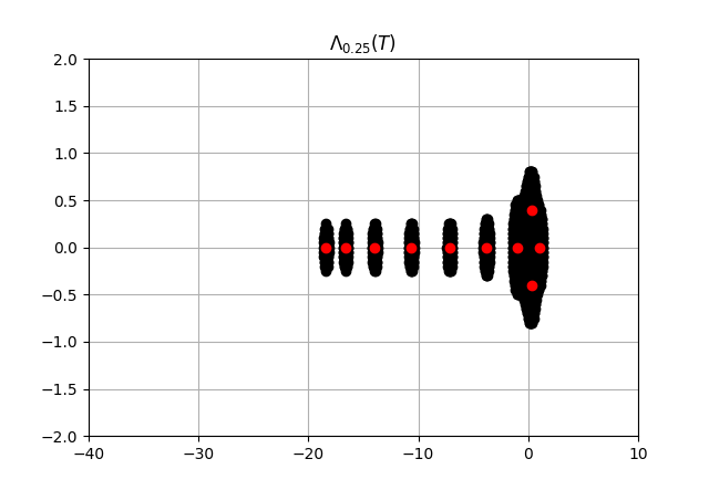
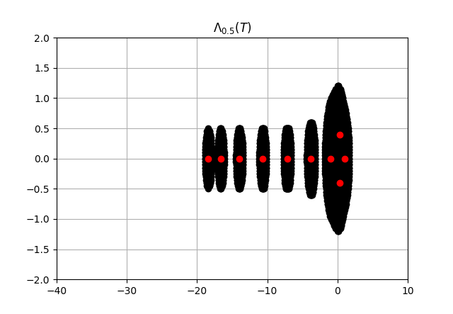
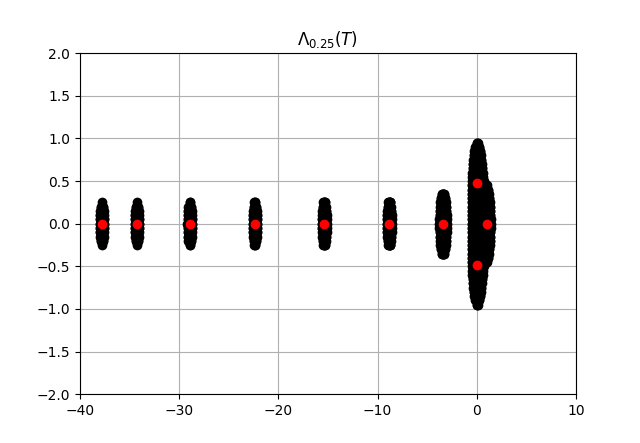
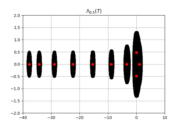
The pseudospectra is used to measure the departure from normality or self-adjoint. In Theorem 4.1, we have seen that the pseudospectra of the heat operator pencil $(A,B)$ is contained in the pseudospectra of the self-adjoint operator $D^{2}$ . The plots of pseudospectra of the discretized one-dimensional heat equation behave in a well-mannered way towards the negative real axis, and we have observed that the eigenvalues away from the origin are less sensitive to perturbations.

References

[1] E. B. Davies, Pseudospectra of differential operators, J. Operator Theory 43 (2000), no. 2, 243–262. MR1753408
[2] J. L. Doob, A probability approach to the heat equation, Trans. Amer. Math. Soc. 80 (1955), 216–280. MR0079376
[3] T. A. Driscoll and L. N. Trefethen, Pseudospectra for the wave equation with an absorbing boundary, J. Comput. Appl. Math. 69 (1996), no. 1, 125–142. MR1391615
[4] A. C. Hansen, On the approximation of spectra of linear operators on Hilbert spaces, J. Funct. Anal. 254 (2008), no. 8, 2092–2126. MR2402104
[5] A. C. Hansen, On the solvability complexity index, the $n$ -pseudospectrum and approximations of spectra of operators, J. Amer. Math. Soc. 24 (2011), no. 1, 81–124. MR2726600
[6] A. Jeribi, Spectral theory and applications of linear operators and block operator matrices, Springer, Cham, 2015. MR3408559
[7] T. Kato, Perturbation theory for linear operators, reprint of the 1980 edition, Classics in Mathematics, Springer, Berlin, 1995. MR1335452
[8] E. Kreyszig, Introductory functional analysis with applications, Wiley Classics Library, John Wiley & Sons, Inc., New York, 1989. MR0992618
[9] G. Krishna Kumar and Judy Augustine, A pseudospectral mapping theorem for operator pencils, Oper. Matrices 16 (2022), no. 3, 709–732. MR4502031
[10] A. S. Markus, Introduction to the spectral theory of polynomial operator pencils, translated from the Russian by H. H. McFaden, translation edited by Ben Silver, Translations of Mathematical Monographs, 71, Amer. Math. Soc., Providence, RI, 1988. MR0971506
[11] R. J. Nagel, Towards a “matrix theory” for unbounded operator matrices, Math. Z. 201 (1989), no. 1, 57–68. MR0990188
[12] E. Rama, A. Chandulal and K. Sambaiah, Application of variational iteration method to obtain the solution of one dimensional heat equation and heat-like equations with variable coefficients, Malaya J. Mat. 9 (2021), no. 1, 996–999. MR4275198
[13] S. C. Reddy, Pseudospectra of operators and discretization matrices and an application to stability of the method of lines, ProQuest LLC, Ann Arbor, MI, 1991. MR2716352
[14] S. C. Reddy and L. N. Trefethen, Pseudospectra of the convection-diffusion operator, SIAM J. Appl. Math. 54 (1994), no. 6, 1634–1649. MR1301275
[15] S. C. Reddy, P. J. Schmid and D. S. Henningson, Pseudospectra of the Orr-Sommerfeld operator, SIAM J. Appl. Math. 53 (1993), no. 1, 15–47. MR1202838
[16] M. S. Sahimi et al., Parabolic-elliptic correspondence of a three-level finite difference approximation to the heat equation, Bull. Malays. Math. Sci. Soc. (2) 26 (2003), no. 1, 79–85. MR2055768
[17] V. S. Sunder, Functional analysis, Birkhäuser Advanced Texts: Basler Lehrbücher., Birkhäuser Verlag, Basel, 1997. MR1646508
[18] L. N. Trefethen and M. Embree, Spectra and pseudospectra, Princeton University Press, Princeton, NJ, 2005. MR2155029
[19] L. N. Trefethen, Pseudospectra of linear operators, SIAM Rev. 39 (1997), no. 3, 383–406. MR1469941
[20] L. N. Trefethen, Approximation theory and numerical linear algebra, in Algorithms for approximation, II (Shrivenham, 1988), 336–360, Chapman and Hall, London. MR1071991
[21] C. Tretter, Spectral theory of block operator matrices and applications, Imp. Coll. Press, London, 2008. MR2463978
[22] M. Zlámal, A finite element solution of the nonlinear heat equation, RAIRO Anal. Numér. 14 (1980), no. 2, 203–216. MR0571315

	$\displaystyle\lambda\in\Lambda_{n,\epsilon}(\alpha A,\alpha B)\setminus\sigma(\alpha A,\alpha B)$	$\displaystyle\Longleftrightarrow\left\\|(\lambda\alpha B-\alpha A)^{-2^{n}}\right\\|^{\frac{1}{2^{n}}}\geq\epsilon^{-1}$
		$\displaystyle\Longleftrightarrow\left\\|(\lambda B-A)^{-2^{n}}\right\\|^{\frac{1}{2^{n}}}\geq\frac{\|\alpha\|}{\epsilon}$
		$\displaystyle\Longleftrightarrow\lambda\in\Lambda_{n,\frac{\epsilon}{\|\alpha\|}}(A,B)\setminus\sigma(A,B).$

	$\displaystyle\lambda\in\Lambda_{n,\epsilon}(\beta A+\alpha B,B)\setminus\sigma(\beta A+\alpha B,B)$	$\displaystyle\Longleftrightarrow\left\\|(\lambda B-\beta A-\alpha B)^{-2^{n}}\right\\|^{\frac{1}{2^{n}}}\geq\epsilon^{-1}$
		$\displaystyle\Longleftrightarrow\ \frac{1}{\|\beta\|}\left\\|\left(\frac{\lambda-\alpha}{\beta}B-A\right)^{-2^{n}}\right\\|^{\frac{1}{2^{n}}}\geq\epsilon^{-1}$
		$\displaystyle\Longleftrightarrow\ \frac{\lambda-\alpha}{\beta}\in\Lambda_{n,\frac{\epsilon}{\|\beta\|}}(A,B)\setminus\sigma(A,B)$
		$\displaystyle\Longleftrightarrow\ \lambda\in\alpha+\beta\,\Lambda_{n,\frac{\epsilon}{\|\beta\|}}(A,B)\setminus\sigma(A,B).$

	$\displaystyle\left\\|\begin{pmatrix}I&G_{2}(\lambda)^{2^{n}}\\ &I\end{pmatrix}\right\\|$	$\displaystyle=\left\\|\begin{pmatrix}I&\left(\left(\lambda B_{1}-A_{1}\right)^{-1}\left(\lambda B_{2}-A_{2}\right)\right)^{2^{n}}\\ &I\end{pmatrix}\right\\|$
		$\displaystyle\leq\left\\|\begin{pmatrix}I&\\ &I\end{pmatrix}\right\\|+\left\\|\begin{pmatrix}&&\left(\left(\lambda B_{1}-A_{1}\right)^{-1}\left(\lambda B_{2}-A_{2}\right)\right)^{2^{n}}\\ &&\end{pmatrix}\right\\|$
		$\displaystyle\leq 1+\left\\|\left(\left(\lambda B_{1}-A_{1}\right)^{-1}\left(\lambda B_{2}-A_{2}\right)\right)^{2^{n}}\right\\|.$

	$\displaystyle\left\\|\begin{pmatrix}I&\\ F_{2}(\lambda)^{2^{n}}&I\end{pmatrix}\right\\|$	$\displaystyle=\begin{pmatrix}I&\\ \left(\left(\lambda B_{3}-A_{3}\right)\left(\lambda B_{1}-A_{1}\right)^{-1}\right)^{2^{n}}&I\end{pmatrix}$
		$\displaystyle\leq\left\\|\begin{pmatrix}I&\\ &I\end{pmatrix}\right\\|+\left\\|\begin{pmatrix}&&\\ \left(\left(\lambda B_{3}-A_{3}\right)\left(\lambda B_{1}-A_{1}\right)^{-1}\right)^{2^{n}}&&\end{pmatrix}\right\\|$
		$\displaystyle\leq 1+\left\\|\left(\left(\lambda B_{3}-A_{3}\right)\left(\lambda B_{1}-A_{1}\right)^{-1}\right)^{2^{n}}\right\\|.$

	$\displaystyle\left\\|\left(\left(\lambda B_{1}-A_{1}\right)^{-1}\left(\lambda B_{2}-A_{2}\right)\right)^{2^{n}}\right\\|$	$\displaystyle\leq\left\\|\left(\lambda B_{1}-A_{1}\right)^{-1}\left(\lambda B_{2}-A_{2}\right)\right\\|^{2^{n}}=\delta_{1}^{2^{n}},$
	$\displaystyle\left\\|\left(\left(\lambda B_{3}-A_{3}\right)\left(\lambda B_{1}-A_{1}\right)^{-1}\right)^{2^{n}}\right\\|$	$\displaystyle\leq\left\\|\left(\lambda B_{3}-A_{3}\right)\left(\lambda B_{1}-A_{1}\right)^{-1}\right\\|^{2^{n}}=\delta_{2}^{2^{n}}.$

Pseudospectra of the heat operator pencil

Abstract.

Key words and phrases:

2020 Mathematics Subject Classification:

2020 Mathematics Subject Classification:

1. Introduction

1.1. Background and Outline

Definition 1.1.

2. (n,ϵ)(n,\epsilon)-pseudopsectra of the closed linear operator pencil

Definition 2.1.

Remark 2.2.

Lemma 2.3.

Proof.

Theorem 2.4.

Proof.

Theorem 2.5.

Proof.

Theorem 2.6.

Proof.

Lemma 2.7.

Proof.

Theorem 2.8.

Proof.

Theorem 2.9.

Proof.

Theorem 2.10.

Proof.

Corollary 2.11.

3. Pseudospectra of the 2×22\times 2 unbounded block operator matrix pencil

Theorem 3.1.

Proof.

Theorem 3.2.

Proof.

Theorem 3.3.

Proof.

Theorem 3.4.

Proof.

Theorem 3.5.

Proof.

Theorem 3.6.

Proof.

Theorem 3.7.

Proof.

4. Pseudospectra of the one-dimensional heat operator pencil

4.1. Eigenvalue analysis

4.2. Psuedospectral analysis

Theorem 4.1.

Proof.

Proposition 4.2.

Proof.

Remark 4.3.

4.3. Discretization

References

2. $(n,\epsilon)$ -pseudopsectra of the closed linear operator pencil

3. Pseudospectra of the $2\times 2$ unbounded block operator matrix pencil