Pure Tone Modes
for a Elliptic Drum
1 Expository Lump
In 1868 Émile Mathieu published a memoir showing how to find the modes, often called standing modes, that generate pure tones in the vibration of an elliptic drum of arbitrary aspect ratio [8]. In preparing [1], together with my co-authors Chris Brimacombe and Mair Zamir, I read that memoir in detail; indeed we asked my colleague Robert H. C. Moir to translate the memoir from French in order to make that job easier. We learned that Mathieu had solved the linear model PDE problem completely, and had given a detailed discussion of the possible nodal lines—that is, places on the membrane that would not move if the drum was oscillating in that mode, including a complete zero-counting discussion using Sturm theory, which he extended to the periodic case. But he published no pictures; perhaps he had sketched them for himself, but we know of none that survive from that time. Later authors, of course, have supplied such pictures: see for instance [7] or [2] or [3]. Once one has seen such pictures, Mathieu’s verbal descriptions of the number and location of nodal lines (hyperbolas and ellipses, actually) make more sense. In this note I show some of the pictures I computed for myself using the (somewhat quixotic) software that I wrote for the Mathieu functions and for solving the Mathieu equation.
We parameterize the elliptic geometry as Mathieu did (he credited the change of coordinates to Lamé who called the result “thermometric” coordinates) through what is now called the confocal elliptic coordinates , , or equivalently . The real parameter gives the distance between the foci of the ellipse. These coordinates are singular in the case when the ellipse becomes a circle, which is a bit of a headache: the proper analysis of the reduction to the circular case requires a double limit process (see Appendix B of [1] for a sketch of such an analysis). Mathieu starts with a wave equation, containing a material parameter representing the ratio of stress to density in the membrane, and then by separation of variables with the frequency of oscillation parameter dealing with the physical parameter; here is a solution of the so-called Mathieu differential equation and is a solution of the so-called modified Mathieu equation. These are also called the angular and radial Mathieu equations.
The Mathieu differential equation is
| (1) |
and the modified Mathieu differential equation is
| (2) |
where is a parameter that depends on the focal parameter and the frequency of oscillation ; the parameter is an eigenvalue of the differential equation (1). The eigenvalue depends on the value of , and must be chosen to make the solution periodic with period either or . Mathieu also divided solutions up into even and odd categories, analogous to cosine and to sine. As in [1] we follow Mathieu and denote the Mathieu functions by for the even solutions and for the odd, and the modified Mathieu functions by and . Here is an integer (Mathieu used the letter in this way, and it might seem unusual to modern eyes that are now used to the Fortran I-N convention of single-letter integer variables being , , , , , or ). We have for the even solutions and for the odd. We normalize the eigenfunctions as follows:
| (3) |
We normalize the modified Mathieu functions analogously, so that and . This normalization is used in some places in the literature, but most people use a different one involving the square integral over the period. See [1] for a discussion of why we chose this one.
The frequency of vibration associated with a particular standing mode depends also on the material properties of the membrane as encapsulated in the parameter , the ratio of tension to density in the (homogeneous) membrane. If the membrane is oscillating like then via we have
| (4) |
Some authors use in place of .
It is the so-called modified Mathieu functions and which determine, through the boundary conditions (the membrane is fixed at the edges, so there), the value of . Mathieu established that every natural mode of the membrane is of the form
| (5) |
or
| (6) |
The dependence on the frequency of oscillation can be made clearer by writing a mode in full as
| (7) |
That is, multiple values of are possible for the same PDE with fixed parameter because different modes of vibration can be excited at the same time. Therefore a general solution composed of a sum of different excited modes would be a sum over modes with different values of and therefore of .
If we have a fixed elliptical drum in mind, then it will have a given aspect ratio or equivalently eccentricity. Say, for the sake of argument, that the aspect ratio is . Then we have (putting the major axis on the -axis)
defining the outer boundary of the ellipse (this also defines the units we use): this is quickly solved111 so and . to get and . Part of the attraction of choosing this aspect ratio for demonstration is that the numbers are so simple.
To find the permissible values of that leave the edge of the drum fixed, then, we have to solve either
| (8) |
or
| (9) |
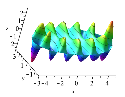
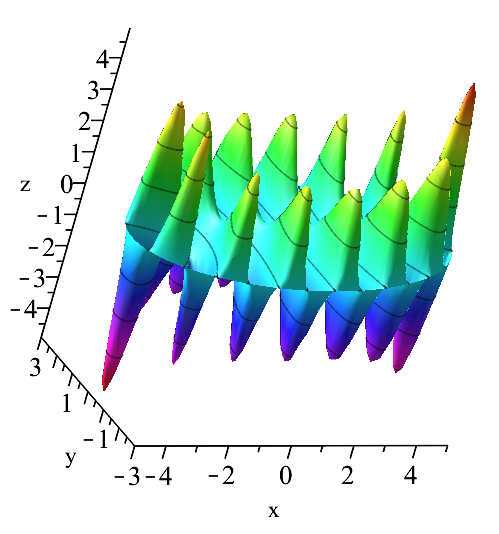
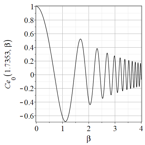
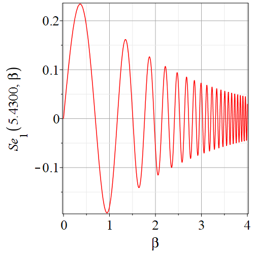
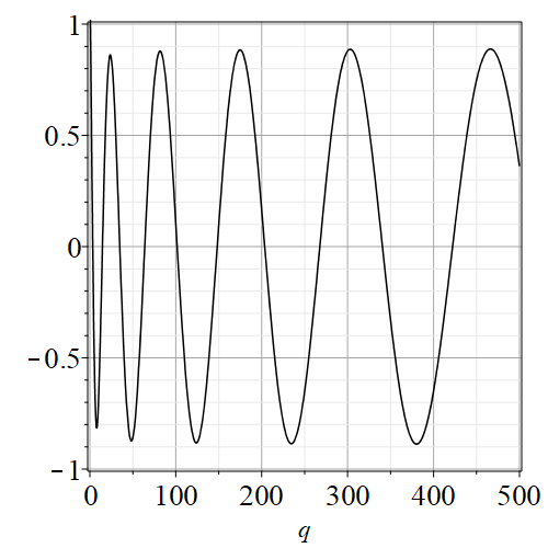
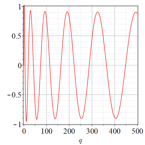
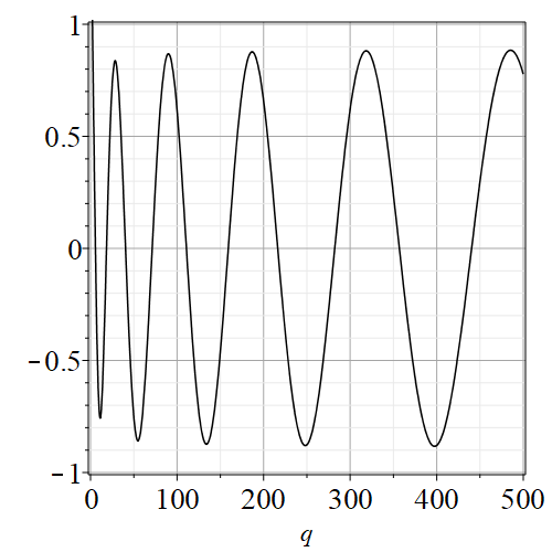
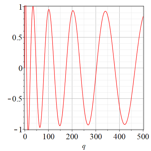
for the parameter . These are (of course) nonlinear equations, and for real values of and turn out always to have an infinite number of solutions, for each value of the index . See figure 1 where we show a representative pair of modified Mathieu equations and see figure 2 where we fix and vary , exhibiting an oscillatory function which apparently has an infinite number of zeros. In practice we are only interested in the first few; the very large values of giving distant zeros will give impractically high-frequency standing modes anyway.
2 Finding numerically
We wish to find, for a given nonnegative integer and choice of “even” or “odd”, the values of for which , where is either (even case) or (odd case) for the appropriate . Either way this is a nonlinear equation in the real parameter that has an infinite number of solutions, as evidenced by figures 2(a)–2(d). In those figures, it is important that we chose to normalize by making while its derivative with respect to was zero there; if instead we had chosen to use the integral normalization then these values seem to decay root-exponentially, i.e. like .
We also wish to find so that is the first zero of the function , and then another value of so that is the second zero, and so on. Each choice of and of “even” versus “odd’ will give a countably infinite number of values of . There is no standard notation for these zeros. For now we will write for the for the value of that makes the th zero of (the even case), for , , , . Similarly we will write for the value of that makes the th zero of (note that for all and we can say this is the th zero, if we like: then here as with the index starts at ).
By trying to plot as a function of for various (we need first to find the appropriate eigenvalue , and how to do this is described in [1] for example) we see that in general increasing brings the first zero closer to the origin. However, the motion of the zeros is not, in general, monotonic. Nonetheless, by simply plotting the function for a few values of one can quickly get an initial estimate of the value of for which .
Once one has a decent initial estimate , one would like to use Newton’s method to find the value of more precisely. This requires derivatives with respect to , which ordinarily would require a Fréchet derivative and the use of a Green’s function (which works perfectly well) but I can report with pleasure that the simple Squire-Trapp formula [9] for numerical differentiation works beautifully here (see [5, p. 479] for a discussion of the excellent numerical properties of this formula). The derivation of the formula is simple: if is analytic and and are real, then
| (10) |
Therefore, taking the imaginary part gives
| (11) |
So all we need to do to compute is to compute near to but with a small purely imaginary perturbation. The formula does require to be analytic because it effectively uses the Cauchy-Riemann equations (here is in fact entire) and requires to be real when is real and to be computed to high relative accuracy in both the real and imaginary part. This holds in our case.
That is, instead of computing with our real value of , we choose an smaller than the square root of machine epsilon (or whatever tolerance we are computing to) and compute instead with ; we use the real part of the answer for and the imaginary part (divided by ) as . Since will then be smaller than machine epsilon, we can ignore the effects of the perturbation on the real part. This is a kind of finite difference formula, but one that for analytic suffers no instability as . Really, it’s ridiculously effective.
We may then use Newton’s method
where the prime now denotes differentiation with respect to . All of the results in tables 1 and 2 were computed in this way. I only report the values of to a few figures; more can be computed on demand.
The eigenvalues and were computed with an even faster iteration, the Inverse Cubic Iteration described in [4], essentially just for fun. The results are not tabulated here because they can be recomputed easily, given .
| first | second | third | fourth | |
|---|---|---|---|---|
| 0 | 1.7353 | 11.356 | 29.795 | 57.011 |
| 1 | 3.3522 | 14.627 | 34.844 | 63.848 |
| 2 | 5.6530 | 18.486 | 40.457 | 71.241 |
| 3 | 8.6576 | 22.968 | 46.658 | 79.201 |
| 4 | 12.368 | 28.100 | 53.463 | 87.754 |
| 5 | 16.779 | 33.913 | 60.891 | 96.903 |
| first | second | third | fourth | |
|---|---|---|---|---|
| 1 | 5.4300 | 19.478 | 42.306 | 73.902 |
| 2 | 7.8189 | 23.636 | 48.248 | 81.626 |
| 3 | 10.803 | 28.363 | 54.775 | 89.914 |
| 4 | 14.406 | 33.696 | 61.800 | 98.762 |
| 5 | 18.637 | 39.642 | 69.499 | 108.17 |
3 Nodal lines
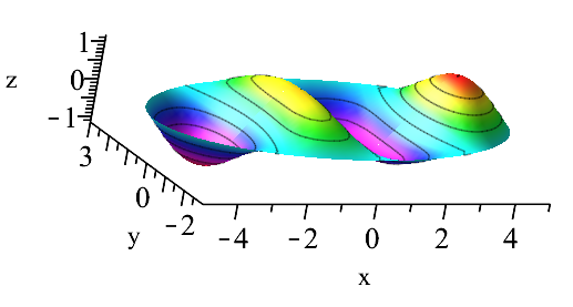
Once one has the values of which are needed, it is straightforward to compute the mode shapes. Somewhat surprisingly, it is awkward to plot them (either in Maple or in Matlab) because the surface is defined parametrically; most contour plotting software wants a regular - grid to work from. In Maple, this can be worked around by using plots[surfdata] which will quickly do a contour plot of irregular data as a decoration of its 3D plots, which can be looked at from the top down (use the keyword orientation=[-90,0] in the plots[surfdata] command). Unfortunately, this is somewhat “too fancy” and does not produce a nice-looking simple 2D contour plot.
Instead, I inverted the coordinate transformation, so , and simply evaluated my numerical solutions of the Mathieu equation (represented as strings of blends [6]) at the resulting and . At low resolution the contour plots take only a few seconds for each one, but take up to about a minute for high resolutions such as a by grid. In contrast, the plots[surfdata] approach only takes about three seconds in total for a similar high-resolution graph. But in the meantime, the code was good enough to allow the production of the contour plots in this paper.
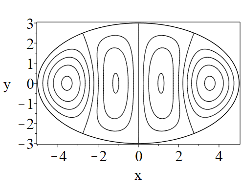
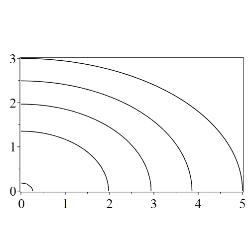
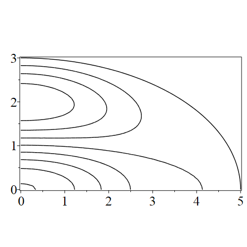
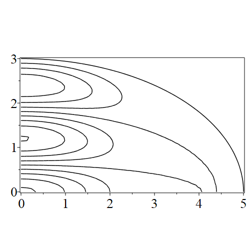
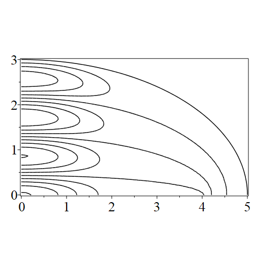
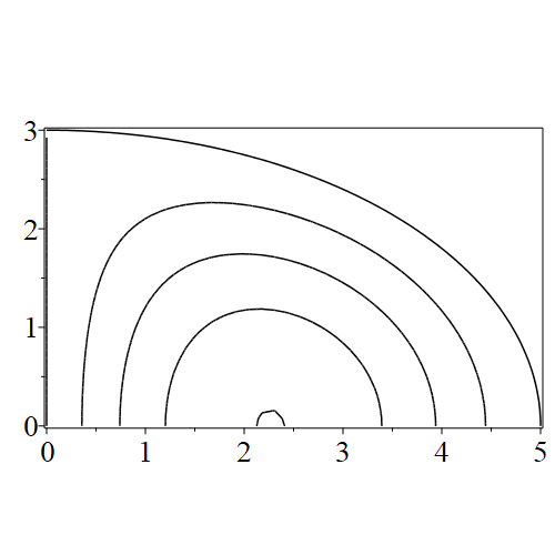
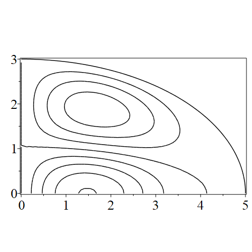
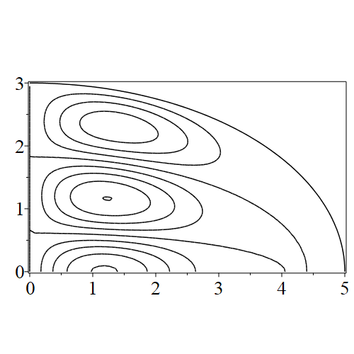
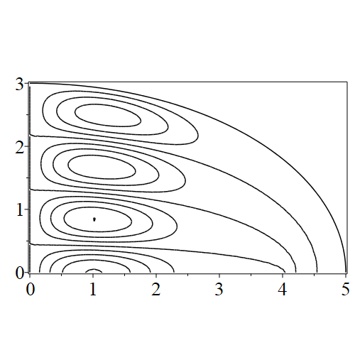
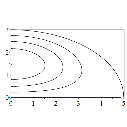
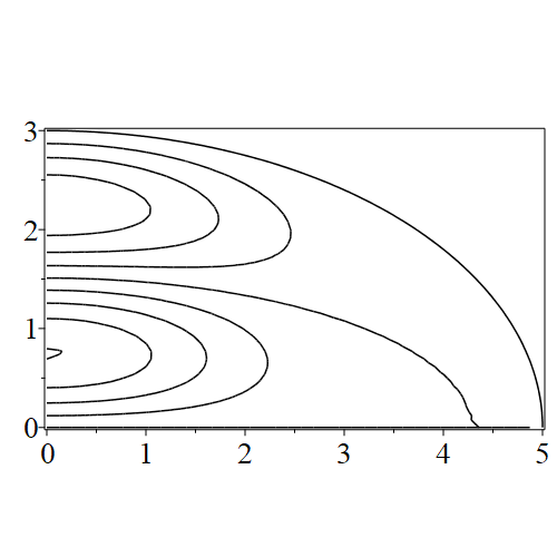
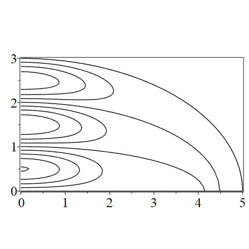
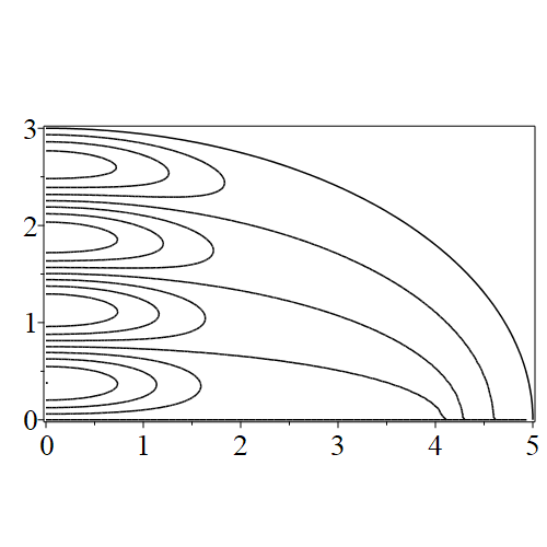
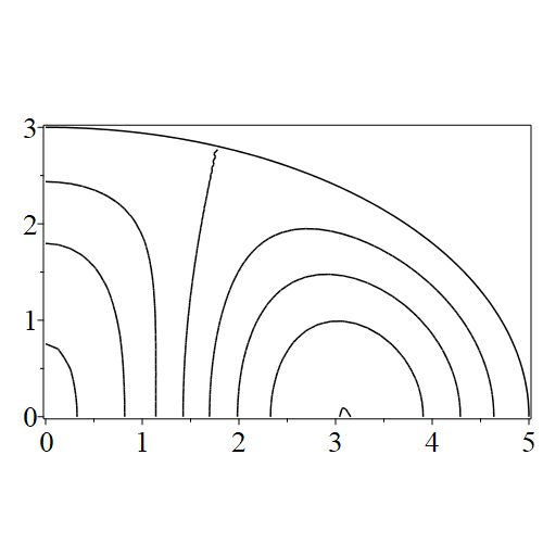
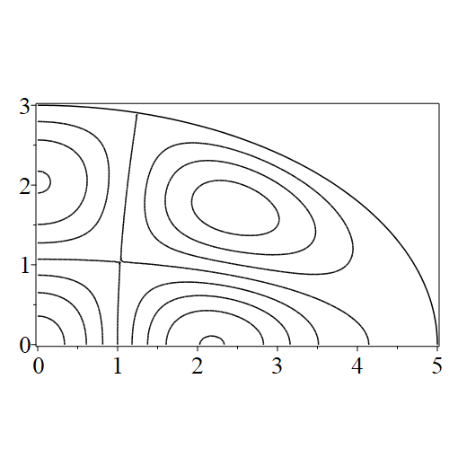
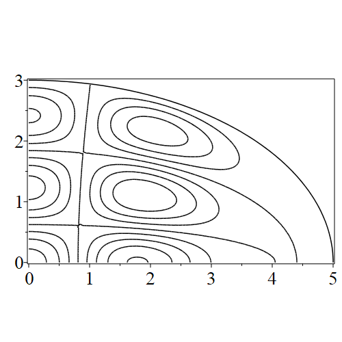
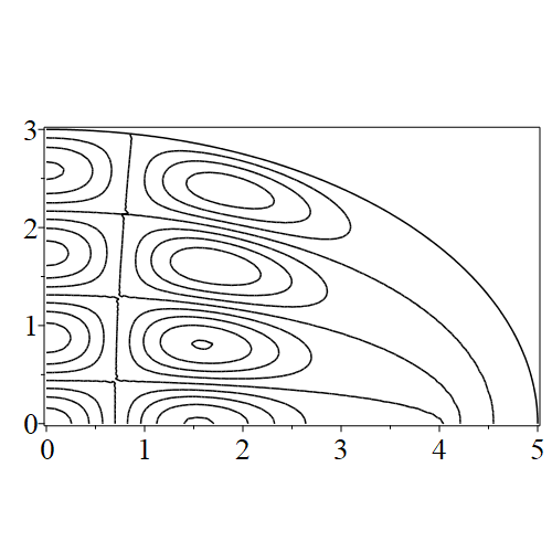
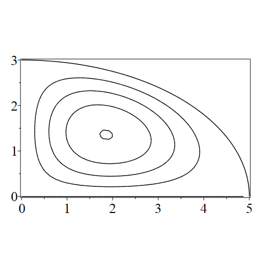
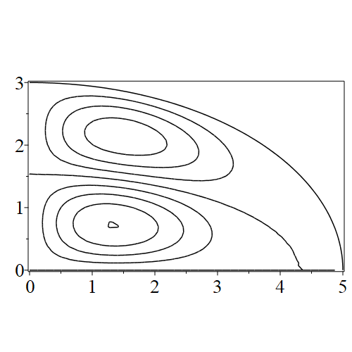
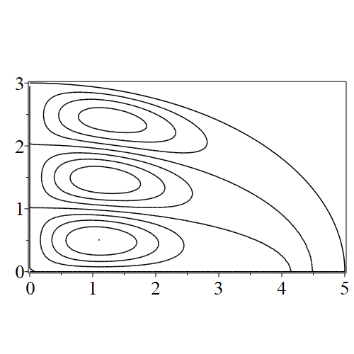
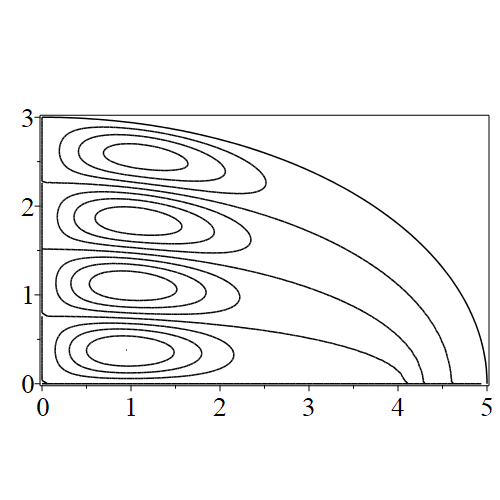
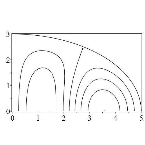
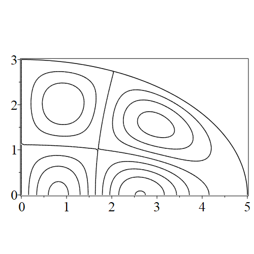
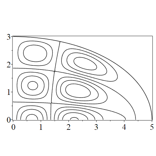
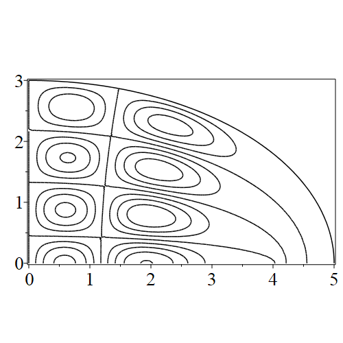
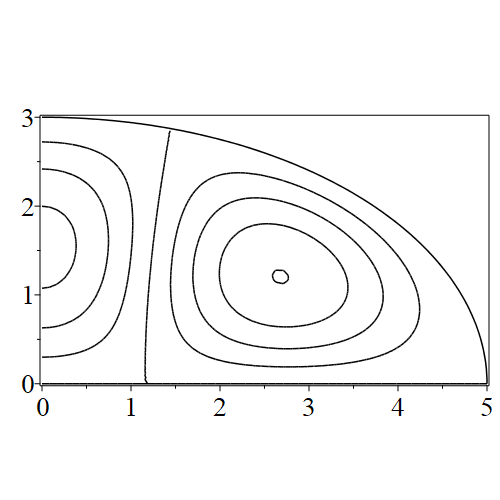
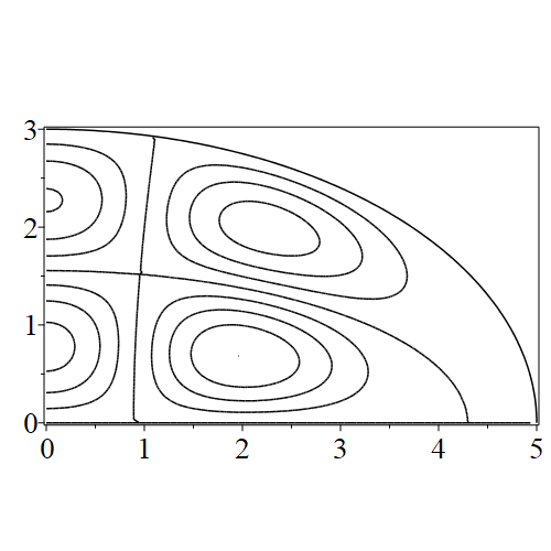
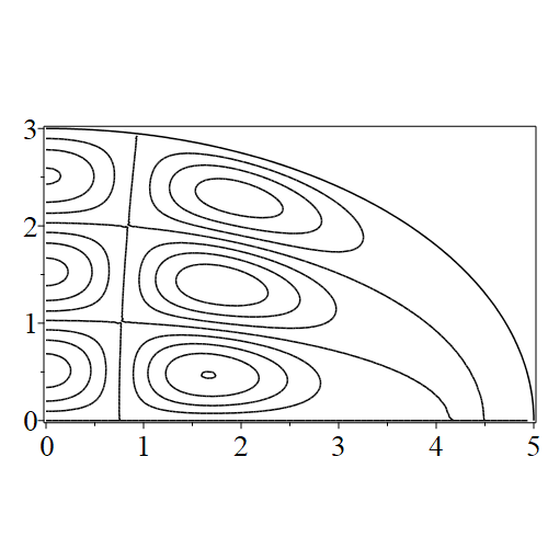
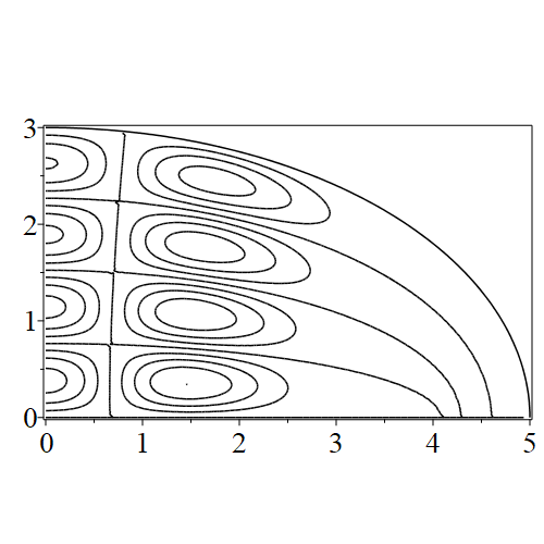
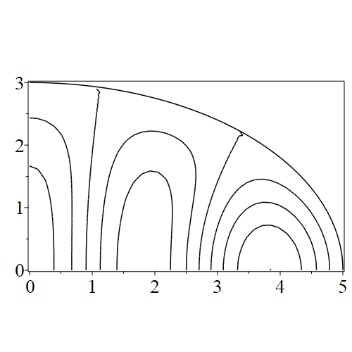
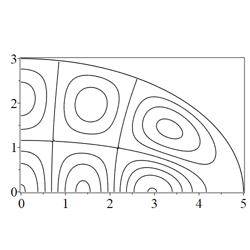
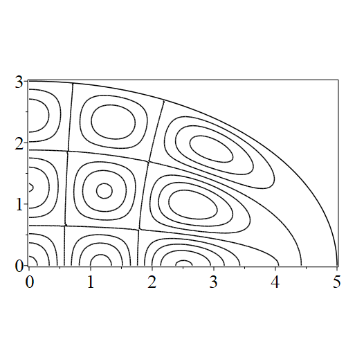
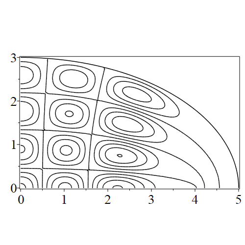
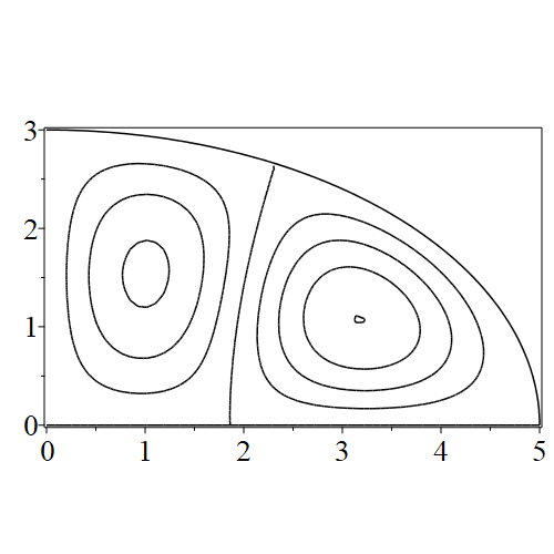
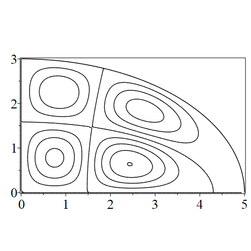
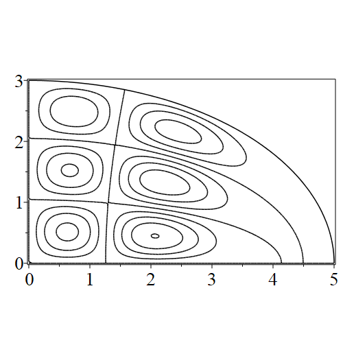
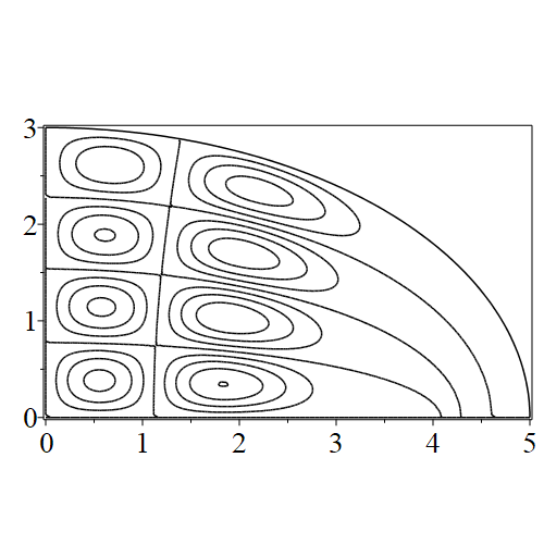
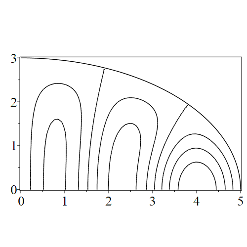
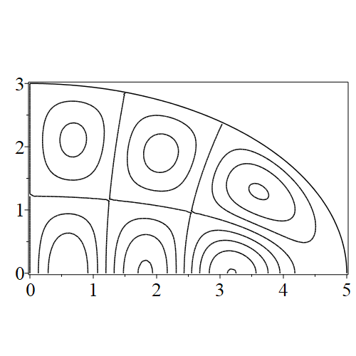
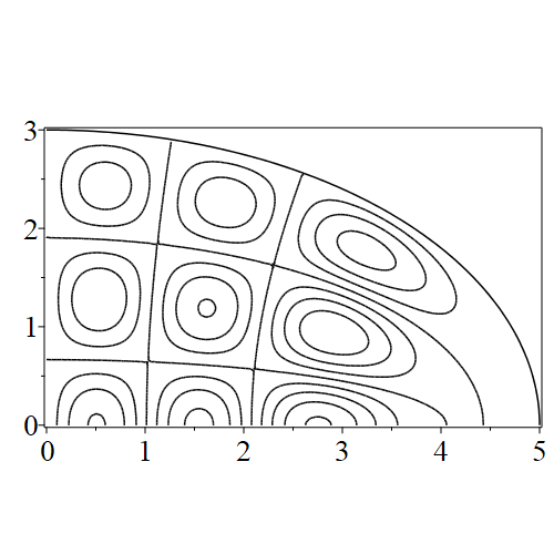
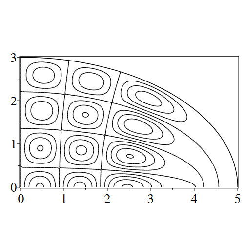
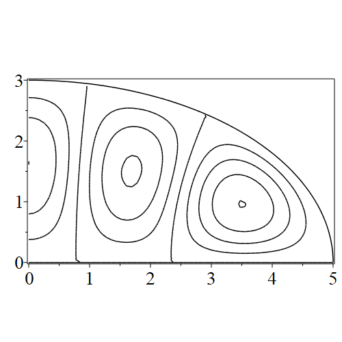
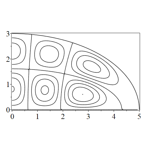
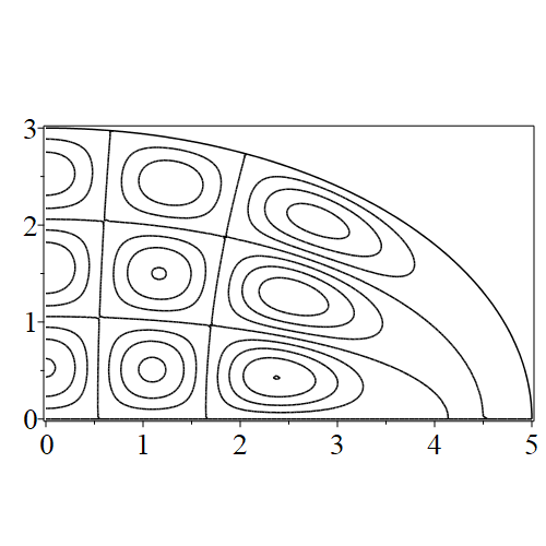
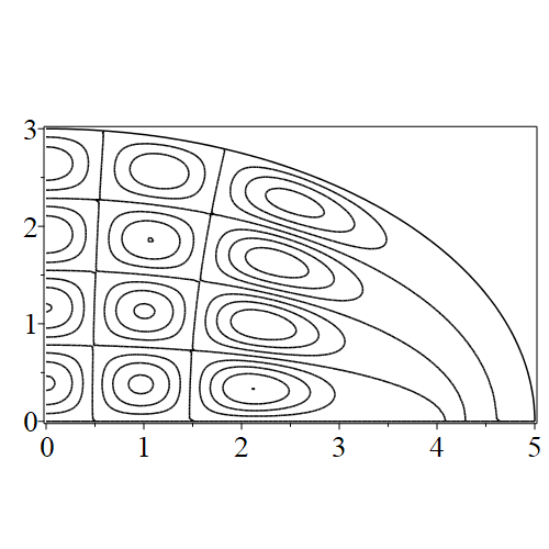
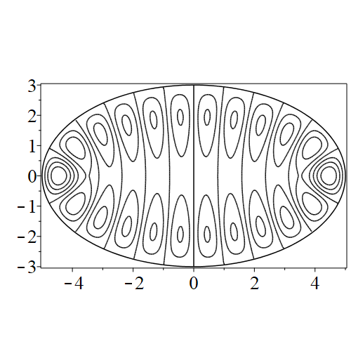
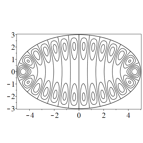
In figure 3 we see the contours corresponding to an even solution with , where the value of was chosen so that was the first zero of . Figures 4–14 plot only the contours of the first quadrant; by symmetry the other three can be deduced. We see confocal elliptic nodal lines, and hyperbolic nodal lines, in several figures; by comparing all the figures we may understand what Mathieu was talking about when he discussed the natural modes of vibration of an elliptic drum.
The paper [3] intriguingly describes “whispering gallery” modes, two of which I plot in figure 15), and “bouncing ball” modes, which seem to be exhibited in the (d) figures corresponding to the fourth zero of all modes plotted in figures 4–14. In a “bouncing ball” mode, most of the vibration is confined to a central channel.
4 Concluding remarks
None of the pictures in this paper would have surprised Mathieu. He predicted the hyperbolic and elliptic nodal lines, and the exact numbers of the hyperbolic lines by an ingenious sign variation argument with Sturm sequences. He also noted that his methods could be used to solve the “confocal elliptic lake” problem—that is, a drum with a confocal hole taken out from the middle, although I did not read his description of the necessary boundary conditions all that closely (these boundary conditions are covered briefly in Chapter 28 of the Digital Library of Mathematical Functions https://dlmf.nist.gov/28 and more thoroughly in [7]).
From the data in tables 1 and 2 we may deduce the frequencies of each of these modes. Writing the general solution as a sum, we have
| (12) |
where the relation ties each frequency to its mode; we have only tabulated the lowest frequency modes in this paper. The unknown coefficients and must be determined by the initial displacement impulse.
References
- [1] Chris Brimacombe, Robert M Corless, and Mair Zamir. Computation and applications of Mathieu functions: A historical perspective. arXiv preprint arXiv:2008.01812, 2020.
- [2] L Chaos-Cador and E Ley-Koo. Mathieu functions revisited: matrix evaluation and generating functions. Revista mexicana de física, 48(1):67–75, 2002.
- [3] Goong Chen, Philip J Morris, and Jianxin Zhou. Visualization of special eigenmode shapes of a vibrating elliptical membrane. SIAM review, 36(3):453–469, 1994.
- [4] Robert M Corless. Inverse cubic iteration. arXiv preprint arXiv:2007.06571, 2020.
- [5] Robert M Corless and Nicolas Fillion. A graduate introduction to numerical methods. Springer-Verlag, 2013.
- [6] Robert M Corless and Erik Postma. Blends in Maple. arXiv preprint arXiv:2007.05041, 2020.
- [7] Julio C Gutiérrez-Vega, RM Rodrıguez-Dagnino, MA Meneses-Nava, and S Chávez-Cerda. Mathieu functions, a visual approach. American Journal of Physics, 71(3):233–242, 2003.
- [8] Émile Mathieu. Mémoire sur le mouvement vibratoire d’une membrane de forme elliptique. Journal de mathématiques pures et appliquées, 13:137–203, 1868.
- [9] William Squire and George Trapp. Using complex variables to estimate derivatives of real functions. SIAM Review, 40(1):pp. 110–112, 1998.