$q$ -Deformations and $t$ -Deformations of the Markov triples

Takeyoshi Kogiso
Department of Mathematics, Josai University,
1-1, Keyakidai Sakado, Saitama, 350-0295, Japan
E-mail address: kogiso@josai.ac.jp

Abstract

In the present paper, we generalize the Markov triples in two different directions. One is generalization in direction of using the $q$ -deformation of rational number introduced by [5] in connection with cluster algebras, quantum topology and analytic number theory. The other is a generalization in direction of using castling transforms on prehomogeneous vector spaces [6] which plays an important role in the study of representation theory and automorphic functions. In addition, the present paper gives a relationship between the two generalizations. This may provide some kind of bridging between different fields.

Introduction

It is well known that Markov triple $(x,y,z)=(\mathrm{Tr}(w(A,B))/3,\mathrm{Tr}(w(A,B)w^{\prime}(A,B))/3,\mathrm{Tr}(w^{\prime}(A,B))/3)$ as a solution of Markov equation $x^{2}+y^{2}+z^{2}=3xyz$ for a triple of Christoffel $ab$ -word $(w(a,b),w(a,b)w^{\prime}(a,b),w^{\prime}(a,b))$ , where $A=\begin{pmatrix}2&1\\ 1&1\end{pmatrix},~{}B=\begin{pmatrix}5&2\\ 2&1\end{pmatrix}$ .

This paper introduces two generalizations of Markov triple in two completely different directions and the relation between them.

Sophie Morier-Genoud and Valentine Ovsienko [5] introduced $q$ -deformation of fractions as the followings. For a positive rational number $\frac{r}{s}=[a_{1},\dots,a_{2m}]=[[c_{1},\dots,c_{r}]]$ , they defined $[a_{1},\dots,a_{2m}]_{q}$ and $[c_{1},\dots,c_{r}]_{q}$ as $q$ -deformation respectively. Furthermore they proved the former coincides with the latter. Thus they defined $[\frac{r}{s}]_{q}:=[a_{1},\dots,a_{2m}]_{q}=[[c_{1},\dots,c_{r}]]_{q}$ as $q$ -deformation of $\frac{r}{s}=[a_{1},\dots,a_{2m}]_{=}[[c_{1},\dots,c_{r}]]$ .

Our first generalization of Markov triples $(h_{w(a,b)}(q),h_{w(a,b)w^{\prime}(a,b)}(q),h_{w^{\prime}(a,b)}(q))$ are given by the properties of $q$ -deformation of a positive fraction. $(x,y,z)=(h_{w(a,b)}(q),h_{w(a,b)w^{\prime}(a,b)}(q),h_{w^{\prime}(a,b)})=(\mathrm{Tr}(w(A_{q},B_{q})/[3]_{q},\mathrm{Tr}(w(A_{q},B_{q})w^{\prime}(A_{q},B_{q}))/[3]_{q},\mathrm{Tr}(w^{\prime}(A_{q},B_{q})/[3]_{q})$ is a solution of $q$ -deformed Markov equation

x^{2}+y^{2}+z^{2}+\frac{(q-1)^{2}}{q^{3}}=[3]_{q}xyz

where $A_{q}=\begin{pmatrix}q+1&q^{-1}\\ 1&q^{-1}\end{pmatrix},~{}B_{q}=\begin{pmatrix}\frac{q^{3}+q^{2}+2q+1}{q}&\frac{q+1}{q}\\ \frac{q+1}{q}&q^{-2}\end{pmatrix}\in SL(2,{\mathbb{Z}}[q,q^{-1}])$ .

On the other hand, Mikio Sato [6] introduced Theory of prehomogeneous vector spaces and classified irreducible prehomogeneous vector spaces with Tatsuo Kimura by using castling transformations of prehomogeneous vector spaces. Our second generalization of Markov triples are given by an application of castling transformations of $t$ -dimensional prehomogeneous vector spaces. We find that a certain subtree of the case for $t=3$ is related to Markov tree of Markov triples $(\mathrm{Tr}(w(A,B))/3,\mathrm{Tr}(w(A,B)w^{\prime}(A,B))/3,\mathrm{Tr}(w^{\prime}(A,B))/3)$ and show that subtree in tree of castling transformation of $t$ -dimensional prehomogeneous vector space corresponds to a tree of triplets $(f_{w}(t),f_{ww^{\prime}}(t),f_{w^{\prime}}(t))$ of polynomials associated to a triple of Christoffel $ab$ -words $(w(a,b),w(a,b)w^{\prime}(a,b),w^{\prime}(a,b))$ . This triple $(x,y,z)=(f_{w(a,b)}(t),f_{w(a,b)w^{\prime}(a,b)}(t),f_{w^{\prime}(a,b)}(t))$ is a solution of a $t$ -deformed Markov equation

x^{2}+y^{2}+z^{2}+(t-3)=txyz.

Moreover there exists a relation $f_{w(a,b)}(q^{-1}[3]_{q})=qh_{w(a,b)}(q)$ between $q$ -deformations and $t$ -deformations.

This paper is organized into the following sections.

In $\S 1$ , properties of $q$ -deformation of continued fractions along [5] is described.

In $\S 2$ , by using $\S 1$ , we defined $q$ -deformation of Markov triples and introduce properties and application of them.

In $\S 3$ , from the view point of castling transformation of prehomogeneous vector spaces, we define castling Markov triples (= $t$ -deformations of Markov triples) and introduce properties of them.

In $\S 4$ , relation between the $q$ -deformations and the $t$ -deformation is described.

1 $q$ -Deformation of continued fractions due to Morier-Genoud and Ovsienko

For a rational number $\frac{r}{s}\in{\mathbb{Q}}$ and that $r,s$ are positive coprime integers. It is well known that $\frac{r}{s}$ has different continued fraction expansions as follows:

\begin{array}[]{lll}\frac{r}{s}&=a_{1}+\cfrac{1}{a_{2}+\cfrac{1}{\ddots+\cfrac{1}{a_{2m}}}}&=[a_{1},a_{2},\dots,a_{2m}]\\ &=c_{1}-\cfrac{1}{c_{2}-\cfrac{1}{\ddots-\cfrac{1}{c_{k}}}}&=[[c_{1},c_{2},\dots,c_{k}]]\end{array}

(1.1)

with $c_{i}\geq 2$ and $a_{i}\geq 1$ , denoted by $[a_{1},\dots,a_{2m}]$ and $[[c_{1},\dots,c_{k}]]$ , respectively. They are usually called regular and negative continued fractions, respectively. Considering an even number of coefficients in the regular expansion and coefficients greater than 2 in the negative expansion make the expansions unique. Sophie Morier-Genord and Valentin Ovsienko [5] introduced $q$ -deformed rationals and $q$ -continued fractions as follows:

Let $q$ be a formal parameter, put

[a]_{p}:=\frac{1-q^{a}}{1-q}

(1.2)

where $a$ is a non-negative integer.

(a)

[a_{1},a_{2},\dots,a_{2m}]_{q}:=[a_{1}]_{q}+\cfrac{q^{a_{1}}}{[a_{2}]_{q^{-1}}+\cfrac{q^{-a_{2}}}{[a_{3}]_{q}+\cfrac{q^{a_{3}}}{[a_{4}]_{q^{-1}}+\cfrac{q^{-a_{4}}}{\cfrac{\ddots}{[a_{2m-1}]_{q}+\cfrac{q^{a_{2m-1}}}{[a_{2m}]_{q^{-1}}}}}}}}

(1.3)

(b)

[[c_{1},c_{2},\dots,c_{k}]]_{q}:=[c_{1}]_{q}-\cfrac{q^{c_{1}-1}}{[c_{2}]_{q}-\cfrac{q^{c_{2}-1}}{[c_{3}]_{q}-\cfrac{q^{c_{3}-1}}{[c_{4}]_{q}-\cfrac{q^{c_{4}-1}}{\cfrac{\ddots}{[c_{k-1}]_{q}-\cfrac{q^{c_{k-1}-1}}{[c_{k}]_{q}}}}}}}

(1.4)

Theorem 1.1.

(Morier-Genoud and Ovsienko [5]) If a rational number $\frac{r}{s}$ has a regular and negative continued fraction expansion form $\frac{r}{s}=[a_{1},\dots,a_{2m}]=[[c_{1},\dots,c_{k}]]$ ,

then

[a_{1},\dots,a_{2m}]_{q}=[[c_{1},\dots,c_{k}]]_{q}=:[\frac{r}{s}]_{q}

(1.5)

Example 1.2.

$[\frac{5}{2}]_{q}=[[3,2]]_{q}=[2,2]_{q}=\frac{1+2q+q^{2}+q^{3}}{1+q}$

$[\frac{5}{3}]_{q}=[[2,3]]_{q}=[1,1,1,1]_{q}=\frac{1+q+2q^{2}+q^{3}}{1+q+q^{2}}$

$[\frac{7}{3}]_{q}=[[3,2,2]]_{q}=[2,3]_{q}=\frac{1+2q+2q^{2}+q^{3}+q^{4}}{1+q+q^{2}}$

$[\frac{7}{4}]_{q}=[[2,4]]_{q}=[1,1,2,1]_{q}=\frac{1+q+2q^{2}+2q^{3}+q^{4}}{1+q+q^{2}+q^{3}}$

$[\frac{7}{5}]_{q}=[[2,2,3]]_{q}=[1,1,2,1]_{q}=\frac{1+q+2q^{2}+2q^{3}+q^{4}}{1+q+2q^{2}+q^{3}}$

Theorem 1.3.

(Morier-Genoud and Ovsienko [5]) The following two matrices

M^{+}_{q}(a_{1},\dots,a_{2m}):=\begin{pmatrix}[a_{1}]_{q}&q^{a_{1}}\\ 1&0\end{pmatrix}\begin{pmatrix}[a_{2}]_{q^{-1}}&q^{-a_{2}}\\ 1&0\end{pmatrix}\cdots\begin{pmatrix}[a_{2m-1}]_{q}&q^{a_{2m-1}}\\ 1&0\end{pmatrix}\begin{pmatrix}[a_{2m}]_{q^{-1}}&-q^{-a_{2m}}\\ 1&0\end{pmatrix}

(1.6)

M_{q}(c_{1},\dots,c_{k}):=\begin{pmatrix}[c_{1}]_{q}&-q^{c_{1}-1}\\ 1&0\end{pmatrix}\begin{pmatrix}[c_{2}]_{q}&-q^{c_{2}-1}\\ 1&0\end{pmatrix}\cdots\begin{pmatrix}[c_{k}-1]_{q}&-q^{c_{k-1}-1}\\ 1&0\end{pmatrix}\begin{pmatrix}[c_{k}]_{q}&-q^{c_{k}-1}\\ 1&0\end{pmatrix}

(1.7)

satisfy the following equations:

(i)

M_{q}^{+}(a_{1},\dots,a_{2m})=\begin{pmatrix}q\mathcal{R}&\mathcal{R}^{\prime}_{2m-1}\\ q\mathcal{S}&\mathcal{S}^{\prime}_{2m-1}\end{pmatrix}

(1.8)

where $\frac{\mathcal{R}(q)}{\mathcal{S}(q)}=[a_{1},a_{2},\dots,a_{2m}]_{q},~{}~{}\frac{\mathcal{R}^{\prime}_{2m-1}(q)}{\mathcal{S}^{\prime}_{2m-1}(q)}=[a_{1},\dots,a_{2m-1}]_{q}$

(ii)

M_{q}(c_{1},\dots,c_{k})=\begin{pmatrix}\mathcal{R}&-q^{c_{k}-1}\mathcal{R}_{k-1}\\ \mathcal{S}&-q^{c_{k}-1}\mathcal{S}^{\prime}_{k-1}\end{pmatrix}

(1.9)

where $\frac{\mathcal{R}(q)}{\mathcal{S}(q)}=[[c_{1},\dots,c_{k}]]_{q},~{}~{}\frac{\mathcal{R}_{k-1}(q)}{\mathcal{S}_{k-1}(q)}=[c_{1},\dots,c_{k-1}]_{q}$

Theorem 1.4.

(Morier-Genoud and Ovsienko [5]) $R_{q}:=\begin{pmatrix}q&1\\ 0&1\end{pmatrix},~{}L_{q}:=\begin{pmatrix}1&0\\ 1&q^{-1}\end{pmatrix},~{}S_{q}:=\begin{pmatrix}0&-q^{-1}\\ 1&0\end{pmatrix}$ , then

M_{q}^{+}(a_{1},\dots,a_{2m})=R_{q}^{a_{1}}L_{q}^{a_{2}}\cdots R_{q}^{a_{2m-1}}L_{q}^{a_{2m}}

(1.10)

and

M_{q}^{+}(c_{1},\dots,c_{k})=R_{q}^{c_{1}}S_{q}R_{q}^{c_{2}}S_{q}\cdots S_{q}R_{q}^{c_{k}}S_{q}.

(1.11)

2 $q$ -Deformations of the Markov equation and Markov triples

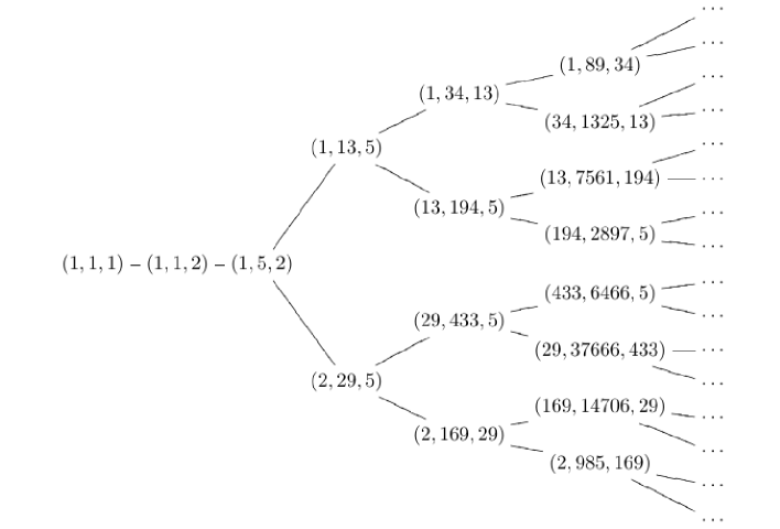
A triple $(x,y,z)$ of positive integers is called Markov triple (up to permutation) when $(x,y,z)$ is a solution of the Markov equation

x^{2}+y^{2}+z^{2}=3xyz.

(2.1)

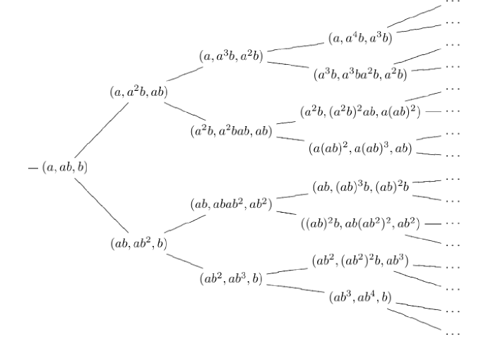
A well-defined set of representative is obtained starting with $(1,1,1),(1,2,1),(1,5,2)$ and then proceeding recursively going from Markov triple $(p,q,r)$ to the new Markov triples $(3qr-p,q,r),(p,3pr-q,r),(p,q,3pq-r)$ (up to permutation). The Markov tree of representatives of Markov triples (Figure 1) and the tree of triples of Christoffel $ab$ -words (Figure2) are well known( cf. [1]).

We consider the following tree of triple of Christoffel $ab$ -words (Cohn word ) form P.201 in [2] corresponding to Markov triples along Bombieri [2] and its modification-version in [1]

Theorem 2.1.

([2], [3], [4]) For $A:=\begin{pmatrix}2&1\\ 1&1\end{pmatrix},B:=\begin{pmatrix}5&2\\ 2&1\end{pmatrix}$ and triple of Christoffel $ab$ -word)

$(w(a,b),w(a,b)w^{\prime}(a,b),w^{\prime}(a,b))$ , a triple of matrices $(w(A,B),w(A,B)w^{\prime}(A,B),w^{\prime}(A,B))$ is called triple of Cohn matrices.

Then

$\frac{1}{3}(\mathrm{Tr}(w(A,B)),\mathrm{Tr}(w(A,B)w^{\prime}(A,B)),\mathrm{Tr}(w^{\prime}(A,B)))=(w(A,B)_{1,2},\{w(A,B)w^{\prime}(A,B)\}_{1,2},w^{\prime}(A,B)_{1,2})$ is a Markov triple.

We obtain the following $q$ -deformation of triple of Cohn matrices and triple of Markov numbers.

Put $A_{q}:=R_{q}L_{q}=\begin{pmatrix}q+1&q^{-1}\\ 1&q^{-1}\end{pmatrix},~{}B_{q}:=R_{q}^{2}L_{q}^{2}=\begin{pmatrix}\frac{q^{3}+q^{2}+2q+1}{q}&\frac{q+1}{q^{2}}\\ \frac{q+1}{q}&q^{-2}\end{pmatrix}\in SL(2,{\mathbb{Z}}[q,q^{-1}])$ .

Lemma 2.2.

Let $(M,MN,N)$ be a triple of $q$ -deformation of Cohn matrices corresponding Christoffel $ab$ -word triple $(w_{1}(a,b),w_{1}(a,b)w_{2}(a,b),w_{2}(a,b))$ such that

(M,MN,N)=(w_{1}(A_{q},B_{q}),w_{1}(A_{q},B_{q})w_{2}(A_{q},B_{q}),w_{2}(A_{q},B_{q})).

(2.2)

Then the following relation holds.

\mathrm{Tr}(MNM^{-1}N^{-1})+2=-\frac{(q-1)^{2}}{q^{3}}[3]_{q}^{2}

(2.3)

Proof..

In general, the following relation holds for a matrix relation $P=XQ$ ,

\mathrm{Tr}([P,Q])=\mathrm{Tr}([P^{-1},Q^{-1}])=\mathrm{Tr}(P^{-1}Q^{-1}PQ)=\mathrm{Tr}(Q^{-1}X^{-1}Q^{-1}XQQ)=\mathrm{Tr}(X^{-1}Q^{-1}XQ)=\mathrm{Tr}([X,Q]).

(2.4)

Similarly, for $Q=PX$ , $\mathrm{Tr}([P,Q])=\mathrm{Tr}([P,X])$ .

By applying this relation to $q$ -Markov Cohn matrices triple $(w(A_{q},B_{q}),w(A_{q},B_{q})w^{\prime}(A_{q},B_{q}),w^{\prime}(A_{q},B_{q}))$ repeatedly, it is possible to reduce the initial relation to the simplest relation as follows:

\mathrm{Tr}([w(A_{q},B_{q}),w^{\prime}(A_{q},B_{q})])+2=\mathrm{Tr}([A_{q},B_{q}])+2=-\frac{(q-1)^{2}[3]_{q}^{2}}{q^{3}}

(2.5)

∎

Similarly we can obtain the following Lemma form the proof of Lemma 2.2.

Lemma 2.3.

Let $(M,MN,N)$ be $q$ -Markov Cohn matrices triple and put $X:=\begin{pmatrix}m_{1,1}&m_{1,2}\\ m_{2,1}&m_{2,2}\end{pmatrix}\in\{M,MN,N\}$

then we obtain

(1)

\mathrm{Tr}(X)/[3]_{q}=m_{1,2}-(q-1)m_{2,2}\in{\mathbb{Z}}[q,q^{-1}]

(2.6)

(2)

\mathrm{Tr}(X)\in[3]_{q}{\mathbb{Z}}[q,q^{-1}]

(2.7)

(3)

m_{1,2}=(q-1)m_{2,2}+\mathrm{Tr}(X)/[3]_{q}.

(2.8)

Theorem 2.4.

Put $A_{q}:=\begin{pmatrix}q+1&q^{-1}\\ 1&q^{-1}\end{pmatrix},~{}B_{q}:=\begin{pmatrix}\frac{q^{3}+q^{2}+2q+1}{q}&\frac{q+1}{q^{2}}\\ \frac{q+1}{q}&q^{-2}\end{pmatrix}\in SL(2,{\mathbb{Z}}[q,q^{-1}])$ .

Then we have the followings:

For triples Christoffel $ab$ -words $(w(a,b),w(a,b)w^{\prime}(a,b),w^{\prime}(a,b)),$

$(x,y,z)=(\mathrm{Tr}w(A_{q},B_{q})/[3]_{q},\{\mathrm{Tr}\{w(A_{q},B_{q})w^{\prime}(A_{q},B_{q})\}\}/[3]_{q},\mathrm{Tr}w^{\prime}(A_{q},B_{q})/[3]_{q})$

$=:(h_{w(a,b)}(q),h_{w(a,b)w^{\prime}(a,b)}(q),h_{w^{\prime}(a,b)}(q))\in{\mathbb{Z}}[q,q^{-1}]^{3}$

is a solution of the following equation:

x^{2}+y^{2}+z^{2}+\frac{(q-1)^{2}}{q^{3}}=[3]_{q}xyz

(2.9)

Proof..

Fricke identity holds on $SL(2,{\mathbb{Z}}[q,q^{-1}]$ as follows:

\mathrm{Tr}(X)^{2}+\mathrm{Tr}(XY)^{2}+\mathrm{Tr}(Y)^{2}=\mathrm{Tr}(X)\mathrm{Tr}(XY)\mathrm{Tr}(Y)+\mathrm{Tr}(XYX^{-1}Y^{-1})+2

(2.10)

By using Lemma 2.2 and Lemma 2.3, we obtain

$(x,y,z)=(\mathrm{Tr}(w(A_{q},B_{q})/[3]_{q},\mathrm{Tr}(ww^{\prime}(A_{q},B_{q}))/[3]_{q},\mathrm{Tr}(w^{\prime}(A_{q},B_{q}))/[3]_{q})\in{\mathbb{Z}}[q,q^{-1}]^{3}$ is a solution of the $q$ -deformed Markov equation $x^{2}+y^{2}+z^{2}+\frac{(q-1)^{2}}{q^{3}}=[3]_{q}xyz$ ∎

Remark 2.5.

$(x,y,z)=([3]_{q}h_{w}(q),[3]_{q}f_{ww^{\prime}}(q),[3]_{q}h_{w^{\prime}}(q))$

$=(\mathrm{Tr}w(A_{q},B_{q}),\mathrm{Tr}w(A_{q},B_{q})w^{\prime}(A_{q},B_{q}),\mathrm{Tr}(w^{\prime}(A_{q},B_{q}))\in([3]_{q}{\mathbb{Z}}[q,q^{-1}])^{3}$ is a solution of the equation

x^{2}+y^{2}+z^{2}+\frac{(q-1)^{2}[3]_{q}^{2}}{q^{3}}=xyz

(2.11)

Theorem 2.6.

$(x,y,z)=(a_{q},b_{q},c_{q})$ is a solution of

x^{2}+y^{2}+z^{2}+\frac{(q-1)^{2}}{q^{3}}=[3]_{q}xyz

(2.12)

Then

$(\tilde{x},y,z)=([3]_{q}b_{q}c_{q}-a_{q},b_{q},c_{q}),(x,\tilde{y},z)=(a_{q},[3]_{q}a_{q}c_{q}-b_{q},c_{q}),(x,y,\tilde{z})=(a_{q},b_{q},[3]_{q}a_{q}b_{q}-c_{q})$ are also solutions of the equation $(2.12)$

Proof..

$\tilde{x}^{2}+y^{2}+z^{2}+\frac{(q-1)^{2}}{q^{3}}=([3]_{q}b_{q}c_{q}-a_{q})^{2}+b_{q}^{2}+c_{q}^{2}+\frac{(q-1)^{2}}{q^{3}}$

$=[3]q^{2}b_{q}^{2}c_{q}^{2}-2[3]_{q}a_{q}b_{q}c_{q}+\{a_{q}^{2}+b_{q}^{2}+c_{q}^{2}+\frac{(q-1)^{2}}{q^{3}}\}$

$=[3]_{q}^{2}b_{q}c_{q}-[3]_{q}a_{q}b_{q}c_{q}=[3]_{q}([3]_{q}b_{q}c_{q}-a_{q})b_{q}c_{q}=[3]_{q}\tilde{x}yz$

Then $(\tilde{x},y,z)$ is also a solution of $(2.12)$ . Similarly $(x,\tilde{y},z),(x,y,\tilde{z})$ are also solutions of $(2.12)$ . ∎

Remark 2.7.

In classical situation, a Markov triple $(a,b,c)$ is orthogonal to $(a-3bc,b,c)$ as 3-dimensional vectors. However for a solution $(a_{q},b_{q},c_{q})$ of the equation $(2.12)$ , we consider usual inner product $(\cdot,\cdot)$ on ${\mathbb{R}}^{3}$ . Then, since $((a_{q},b_{q},c_{q}),(a_{q}-[3]_{q}b_{q}c_{q},b_{q},c_{q}))=a_{q}^{2}+b_{q}^{2}+c_{q}^{2}-[3]_{q}a_{q}b_{q}c_{q}=-\frac{(q-1)^{2}}{q^{3}}\neq 0,$ $(a_{q},b_{q},c_{q})$ is not orthogonal to $(a_{q}-[3]_{q}b_{q}c_{q})$ for usual inner product.However, since $~{}~{}(\rightarrow 0~{}(q\rightarrow 0))$ , the inner product is near to orthogonal.

Example 2.8.

$h_{a^{3}b}(q)^{2}+h_{a^{3}ba^{2}b}(q)^{2}+h_{a^{2}b}(q)^{2}+\frac{(q-1)^{2}}{q^{3}}$

$=\frac{\mathrm{tr}(A_{q}^{3}B_{q})}{[3]_{q}}^{2}+\frac{\mathrm{tr}(A_{q}^{3}B_{q}A_{q}^{2}B_{q})}{[3]_{q}}^{2}+\frac{\mathrm{tr}(A_{q}^{2}B_{q})}{[3]_{q}}^{2}+\frac{(q-1)^{2}}{q^{3}}$ .

$=\{\frac{\left({q}^{2}+1\right)\left({q}^{6}+3\,{q}^{5}+3\,{q}^{4}+3\,{q}^{3}+3\,{q}^{2}+3\,q+1\right)}{{q}^{5}}\}^{2}$

$+\{\frac{\left({q}^{4}+{q}^{3}+{q}^{2}+q+1\right)\left({q}^{12}+5\,{q}^{11}+12\,{q}^{10}+22\,{q}^{9}+32\,{q}^{8}+39\,{q}^{7}+43\,{q}^{6}+39\,{q}^{5}+32\,{q}^{4}+22\,{q}^{3}+12\,{q}^{2}+5\,q+1\right)}{{q}^{9}}\}^{2}$

$+\{\frac{{q}^{4}+{q}^{3}+{q}^{2}+q+1}{{q}^{3}}\}^{2}+\frac{(q-1)^{2}}{q^{3}}$

$=[3]_{q}\{\frac{\left({q}^{2}+1\right)\left({q}^{6}+3\,{q}^{5}+3\,{q}^{4}+3\,{q}^{3}+3\,{q}^{2}+3\,q+1\right)}{{q}^{5}}\}$

$\{\frac{\left({q}^{4}+{q}^{3}+{q}^{2}+q+1\right)\left({q}^{12}+5\,{q}^{11}+12\,{q}^{10}+22\,{q}^{9}+32\,{q}^{8}+39\,{q}^{7}+43\,{q}^{6}+39\,{q}^{5}+32\,{q}^{4}+22\,{q}^{3}+12\,{q}^{2}+5\,q+1\right)}{{q}^{9}}\}$

$\{\frac{{q}^{4}+{q}^{3}+{q}^{2}+q+1}{{q}^{3}}\}$

$=[3]_{q}\frac{\mathrm{tr}(A_{q}^{3}B_{q})}{[3]_{q}}\frac{\mathrm{tr}(A_{q}^{3}B_{q}A_{q}^{2}B_{q})}{[3]_{q}}\frac{\mathrm{tr}(A_{q}^{2}B_{q})}{[3]_{q}}=[3]_{q}h_{a^{3}b}(q)h_{a^{3}ba^{2}b}(q)h_{a^{2}b}(q)$

2.1 An application of $q$ -Markov triples to fixed points of associated Cohn matrices

Here we introduce an application of $q$ -deformation of Markov triples $(h_{w(a,b)}(q),h_{w(a,b)w^{\prime}(a,b)}(q),h_{w^{\prime}(a.b)}(q))$ to fixed point of $q$ -Cohn matrix $w(A_{q},B_{q})w^{\prime}(A_{q},B_{q})$ .

In Theorem 16 of [2], Bombieri proved a nice properties of Cohn matrix coming from Christoffel $ab$ -words and applied to quadratic irrational number. The following theorem is related to $q$ -quadratic irrational number and $q$ -Cohn matrix $w(A_{q},B_{q})$ for Christoffel $ab$ -word $w(a,b)$ .

Theorem 2.9.

For fixed point $\theta_{q}(w(a,b))$ of linear fractional transformation with respect to $q$ -Cohn matrix $w(A_{q},B_{q})$ corresponding to Christoffel $ab$ -word $w(a,b)$ , we obtain

\theta_{q}(w(a,b))=[\overline{\Pi}]_{q}.

(2.13)

by using a finite sequence $\Pi$ that is obtained by substituting

a\mapsto 1,1,~{}~{}b\mapsto 2,2.

(2.14)

Proof..

From the definition of $q$ -rational number $[\frac{r}{s}]_{q}=[a_{1},\dots,a_{2m}]_{q}=[[c_{1},\dots,c_{k}]]_{q}$ and $\frac{w(A_{q},B_{q})_{1,1}}{w(A_{q},B_{q})_{2,1}}=[a_{1},\dots,a_{2m}]_{q}$ due to Theorem1.3 and Theorem1.4 , we can transform the relation $w(A_{q},B_{q})\cdot\theta_{q}(w(a,b))=\theta_{q}(w(a,b))$ to

\theta_{q}(w(a,b)):=[a_{1}]_{q}+\cfrac{q^{a_{1}}}{[a_{2}]_{q^{-1}}+\cfrac{q^{-a_{2}}}{[a_{3}]_{q}+\cfrac{q^{a_{3}}}{[a_{4}]_{q^{-1}}+\cfrac{q^{-a_{4}}}{\cfrac{\ddots}{[a_{2m-1}]_{q}+\cfrac{q^{a_{2m-1}}}{[a_{2m}]_{q^{-1}}+\cfrac{q^{-2m}}{\theta_{q}(w(a,b))}}}}}}}

(2.15)

Then we obtain that $\theta(w(a,b))=[\overline{a_{1},\dots,a_{2m}}]_{q}$

On the other hand, the definition of $A_{q}$ and $B_{q},$ $A_{q}=R_{q}L_{q}=\begin{pmatrix}[1,1]_{q}&q^{-1}\\ 1&q^{-1}\end{pmatrix}$ and $B_{q}=R_{q}^{2}L_{q}^{2}=\begin{pmatrix}q^{-1}[2,2]_{q}&q^{-2}[2]_{q}\\ q^{-1}[2]_{q}&q^{-2}\end{pmatrix}$ . Thus we have $\theta_{q}(w(a,b))=[\overline{\Pi}]_{q}$ , where $\theta_{q}(w(a,b))=[\overline{\Pi}]_{q},$ we here $\Pi$ is a finite sequence that obtained by substituting $a\mapsto 1,1,~{}~{}b\mapsto 2,2.$ ∎

Example 2.10.

$\theta_{q}(a^{2}b)=[\overline{1,1,1,1,2,2}]_{q}$

$=\frac{{q}^{8}+3\,{q}^{7}+5\,{q}^{6}+7\,{q}^{5}+5\,{q}^{4}+3\,{q}^{3}+{q}^{2}-q-1}{2q\left({q}^{6}+2\,{q}^{5}+4\,{q}^{4}+4\,{q}^{3}+4\,{q}^{2}+3\,q+1\right)}$

$+\frac{\sqrt{{q}^{16}+6\,{q}^{15}+19\,{q}^{14}+44\,{q}^{13}+81\,{q}^{12}+126\,{q}^{11}+171\,{q}^{10}+204\,{q}^{9}+213\,{q}^{8}+204\,{q}^{7}+171\,{q}^{6}+126\,{q}^{5}+81\,{q}^{4}+44\,{q}^{3}+19\,{q}^{2}+6\,q+1}}{2q\left({q}^{6}+2\,{q}^{5}+4\,{q}^{4}+4\,{q}^{3}+4\,{q}^{2}+3\,q+1\right)}$

Remark 2.11.

The $q$ -polynomial ${q}^{16}+6\,{q}^{15}+19\,{q}^{14}+44\,{q}^{13}+81\,{q}^{12}+126\,{q}^{11}+171\,{q}^{10}+204\,{q}^{9}+213\,{q}^{8}+204\,{q}^{7}+171\,{q}^{6}+126\,{q}^{5}+81\,{q}^{4}+44\,{q}^{3}+19\,{q}^{2}+6\,q+1$ in the square root is vertical symmetry at middle term $213q^{8}$ .

Remark 2.12.

For $q$ -Cohn matrix $C_{q}(w(a,b))=\begin{pmatrix}r_{q}&t_{q}\\ s_{q}&u_{q}\end{pmatrix}$ for Christoffel $ab$ -word $w(a,b)$ .

If $\frac{r_{q}}{s_{q}}\rightarrow\frac{r}{s}$ $(q\rightarrow 1)$ , then we have

$\frac{r}{s}=[w(a,b)|_{a\mapsto 1,1,~{}b\mapsto 2,2}]=[\Pi]$ and $\frac{r_{q}}{s_{q}}=[\frac{r}{s}]_{q}$ .

2.2 Other $q$ -deformations of Markov triples

Proposition 2.13.

For $A_{q}:=\begin{pmatrix}q+1&q^{-1}\\ 1&q^{-1}\end{pmatrix},~{}B_{q}:=\begin{pmatrix}\frac{q^{3}+q^{2}+2q+1}{q}&\frac{q+1}{q^{2}}\\ \frac{q+1}{q}&q^{-2}\end{pmatrix}$

and Christoffel $ab$ -word $w(a,b),w(a,b)w^{\prime}(a,b),w(a,b))$ ,

$(x,y,z,x^{\prime})=w(A_{q},B_{q})_{1,2},\{w(A_{q},B_{q})w^{\prime}(A_{q},B_{q})\}_{1,2},w^{\prime}(A_{q},B_{q})_{1,2},\mathrm{Tr}(w(A_{q},B_{q})/[3]_{q})\in{\mathbb{Z}}[q,q^{-1}]^{3}$ is a solution of the equation:

\frac{1}{q^{3}}x^{2}+y^{2}+z^{2}=[3]_{q}x^{\prime}yz

(2.16)

on ${\mathbb{Z}}[q,q^{-1}]^{3}.$

Proposition 2.14.

For $A_{q}:=\begin{pmatrix}q+1&q^{-1}\\ 1&q^{-1}\end{pmatrix},~{}B_{q}:=\begin{pmatrix}\frac{q^{3}+q^{2}+2q+1}{q}&\frac{q+1}{q^{2}}\\ \frac{q+1}{q}&q^{-2}\end{pmatrix},$

$(x,y,z,y^{\prime},z^{\prime})=$

$(h_{w_{1}(a,b)}(q),h_{w_{1}(a,b)w_{2}(a,b)}(q),h_{w_{2}(a,b)}(q),\left\{(w_{1}(A_{q},B_{q})w_{2}(A_{q},B_{q}))\right\}_{1,2}|_{q\mapsto q^{-1}}\cdot q^{\textrm{deg.}h_{w_{1}(a,b)w_{2}(a,b)}(q)},$ $w_{2}(A_{q},B_{q})_{1,2})$ is a solution of

\frac{1}{q^{3}}x^{2}+y^{2}+z^{2}+\frac{(q-1)^{2}}{q^{3}}=[3]_{q}xy^{\prime}z^{\prime}.

(2.17)

where $h_{w(a,b)}:=\mathrm{Tr}w(A_{q},B_{q})/[3]_{q}$ .

Example 2.15.

For $(w_{1}(a,b),w_{1}(a,b)w_{2}(a,b),w_{2}(a,b))=(a^{3}b,a^{3}ba^{2}b,a^{2}b)$ corresponding to a Markov triple $(34,1325,13)$ ,

$\begin{array}[]{l}w_{1}(A_{q},B_{q})_{1,2}={\frac{{q}^{7}+4\,{q}^{6}+6\,{q}^{5}+7\,{q}^{4}+7\,{q}^{3}+5\,{q}^{2}+3\,q+1}{{q}^{5}}}\\ w_{2}(A_{q},B_{q})_{1,2}={\frac{{q}^{5}+3\,{q}^{4}+3\,{q}^{3}+3\,{q}^{2}+2\,q+1}{{q}^{4}}}\\ \{w_{1}(A_{q},B_{q})w_{2}(A_{q},B_{q})\}_{1,2}:=q^{-9}({q}^{15}+7\,{q}^{14}+23\,{q}^{13}+52\,{q}^{12}+93\,{q}^{11}+138\,{q}^{10}\\ +177\,{q}^{9}+197\,{q}^{8}+194\,{q}^{7}+167\,{q}^{6}+125\,{q}^{5}+81\,{q}^{4}+44\,{q}^{3}+19\,{q}^{2}+6\,q+1).\end{array}$

Then

$\frac{1}{q^{3}}w_{1}(A_{q},B_{q})_{1,2}^{2}+\{w_{1}(A_{q},B_{q})w_{2}(A_{q},B_{q})\}_{1,2}^{2}+w_{2}(A_{q},B_{q})_{1,2}^{2}$

$=q^{-18}({q}^{2}+1)\left({q}^{6}+3\,{q}^{5}+3\,{q}^{4}+3\,{q}^{3}+3\,{q}^{2}+3\,q+1\right)$

$({q}^{15}+7\,{q}^{14}+23\,{q}^{13}+52\,{q}^{12}+93\,{q}^{11}+138\,{q}^{10}+177\,{q}^{9}+197\,{q}^{8}+194\,{q}^{7}$

$+167\,{q}^{6}+125\,{q}^{5}+81\,{q}^{4}+44\,{q}^{3}+19\,{q}^{2}+6\,q+1)({q}^{2}+q+1)({q}^{5}+3\,{q}^{4}+3\,{q}^{3}+3\,{q}^{2}+2\,q+1)$

$=[3]_{q}h_{a^{3}b}(q)\{w_{1}(A_{q},B_{q})w_{2}(A_{q},B_{q})\}_{1,2}w_{2}(A_{q},B_{q})_{1,2}.$

Example 2.16.

For Christoffel $ab$ -word triple $(w_{1}(a,b),w_{1}(a,b)w_{2}(a,b),w_{2}(a,b))$ $=(abab^{2},$ $abab^{2}ab^{2},ab^{2})$ , let corresponding $q$ -Cohn matrices triple be $(w_{1}(A_{q},B_{q}),w_{1}(A_{q},B_{q})w_{2}(A_{q},B_{q}),$ $w_{2}(A_{q},B_{q}))=(A_{q}B_{q}A_{q}B_{q}^{2},A_{q}B_{q}A_{q}B_{q}^{2}A_{q}B_{q}^{2},A_{q}B_{q}^{2})$ ,

then

$h_{abab^{2}}(q):=\mathrm{Tr}(A_{q}B_{q}A_{q}B_{q}^{2})/[3]_{q}=q^{-8}({q}^{14}+4\,{q}^{13}+11\,{q}^{12}+22\,{q}^{11}+36\,{q}^{10}+50\,{q}^{9}+60\,{q}^{8}+65\,{q}^{7}+60\,{q}^{6}+50\,{q}^{5}+36\,{q}^{4}+22\,{q}^{3}+11\,{q}^{2}+4\,q+1)$

$h_{abab^{2}ab^{2}}(q):=\mathrm{Tr}(A_{q}B_{q}A_{q}B_{q}^{2}A_{q}B_{q}^{2})/[3]_{q}=q^{-13}({q}^{2}+1)$

$\cdot({q}^{22}+7\,{q}^{21}+29\,{q}^{20}+87\,{q}^{19}+208\,{q}^{18}+417\,{q}^{17}+724\,{q}^{16}+1114\,{q}^{15}+1540\,{q}^{14}+1931\,{q}^{13}+2206\,{q}^{12}+2305\,{q}^{11}+2206\,{q}^{10}+1931\,{q}^{9}+1540\,{q}^{8}+1114\,{q}^{7}+724\,{q}^{6}+417\,{q}^{5}+208\,{q}^{4}+87\,{q}^{3}+29\,{q}^{2}+7\,q+1)$

$h_{ab^{2}}(q):={\frac{{q}^{8}+2\,{q}^{7}+4\,{q}^{6}+5\,{q}^{5}+5\,{q}^{4}+5\,{q}^{3}+4\,{q}^{2}+2\,q+1}{{q}^{5}}}$

$\frac{1}{q^{3}}h_{abab^{2}}(q)^{2}+h_{abab}(q)^{2}ab^{2})^{2}+h_{ab}(q)^{2})^{2}+\frac{(q-1)^{2}}{q^{3}}$

$=q^{-26}\left({q}^{2}+q+1\right)\left({q}^{2}-q+1\right)$

$\cdot(q+1)({q}^{7}+3\,{q}^{6}+5\,{q}^{5}+6\,{q}^{4}+6\,{q}^{3}+5\,{q}^{2}+2\,q+1)$

$\cdot({q}^{14}+4\,{q}^{13}+11\,{q}^{12}+22\,{q}^{11}+36\,{q}^{10}+50\,{q}^{9}+60\,{q}^{8}+65\,{q}^{7}+60\,{q}^{6}+50\,{q}^{5}+36\,{q}^{4}+22\,{q}^{3}+11\,{q}^{2}+4\,q+1)$

$\cdot({q}^{22}+6\,{q}^{21}+25\,{q}^{20}+75\,{q}^{19}+184\,{q}^{18}+378\,{q}^{17}+675\,{q}^{16}+1063\,{q}^{15}+1501\,{q}^{14}+1913\,{q}^{13}+2217\,{q}^{12}+2341\,{q}^{11}+2255\,{q}^{10}+1982\,{q}^{9}+1582\,{q}^{8}+1142\,{q}^{7}+738\,{q}^{6}+422\,{q}^{5}+209\,{q}^{4}+87\,{q}^{3}+29\,{q}^{2}+7\,q+1)$

$=[3]_{q}h_{abab^{2}}(q)(q^{23}\cdot(A_{q}B_{q}A_{q}B_{q}^{2}A_{q}B_{q}^{2})_{1,2})_{q\mapsto q^{-1}})\cdot(A_{q}B_{q}^{2})_{1,2}.$

3 A relation of castling transformations of 3-dimensional prehomogeneous vector spaces and Markov triplets and the generalization

3.1 Prehomogeneous vector spaces and castling transformations

Let $G$ be a linear algebraic group and $\rho$ its rational representation on a finite dimensional vector space $V$ , all defined over the complex number field ${\mathbb{C}}$ . If $V$ has a Zariski-dense $G$ -orbit ${\mathbb{O}}$ , we call the triplet $(G,\rho,V)$ a prehomogeneous vector space (abbreviated by PV). In this case, we call $v\in{\mathbb{O}}$ a generic point, and the isotropy subgroup $G_{v}=\{g\in G\mid\rho(g)v=v\}$ at $v$ is called a generic isotropy subgroup. We call a prehomogeneous vector space $(G,\rho,V)$ a reductive prehomogeneous vector space if $G$ is reductive. Let $\rho:G\to GL(V)$ be a rational representation of a linear algebraic group $G$ on an $m$ -dimensional vector space $V$ and let $n$ be a positive integer with $m>n$ . A triplet $\mathcal{C}_{1}:=(G\times GL(n),\rho\otimes\Lambda_{1},V\otimes V(n))$ is a prehomogeneous vector space if and only if a triplet $\mathcal{C}_{2}:=(G\times GL(m-n),\rho^{\ast}\otimes\Lambda_{1},V^{\ast}\otimes V(m-n))$ is a prehomogeneous vector space. We say that $\mathcal{C}_{1}$ and $\mathcal{C}_{2}$ are the castling transforms of each other. Two triplets are said to be castling equivalent if one is obtained from the other by a finite number of successive castling transformations. (cf. [6], [7]). Assume that $(G,\rho,V)$ is a prehomogeneous vector space with a Zariski-dense $G$ -orbit ${\mathbb{O}}$ . A non-zero rational function $f(v)$ on $V$ is called a relative invariant if there exists a rational character $\chi:G\to GL(1)$ satisfying $f(\rho(g)v)=\chi(g)f(v)$ for $g\in G$ . In this case, we write $f\leftrightarrow\chi$ . Let $S_{i}=\{v\in V\mid f_{i}(v)=0\}$ $(i=1,\ldots,l)$ be irreducible components of $S:=V\setminus{\mathbb{O}}$ with codimension one. When $G$ is connected, these irreducible polynomials $f_{i}(v)$ $(i=1,\ldots,l)$ are algebraically independent relative invariants and any relative invariant $f(v)$ can be expressed uniquely as $f(v)=cf_{1}(v)^{m_{1}}\cdots f_{l}(v)^{m_{l}}$ with $c\in{\mathbb{C}}^{\times}$ and $m_{1},\ldots,m_{l}\in{\mathbb{Z}}$ . These $f_{i}(v)$ $(i=1,\ldots,l)$ are called the basic relative invariants of $(G,\rho,V)$ .

Example 3.1.

Let a triplet $(SO(3)\times GL(1),\Lambda_{1}\otimes\Lambda_{1},V(3)\otimes V(1))$ be a 3-dimensional prehomogeneous vector space, and hence its castling transform $(SO(3)\times GL(2),\Lambda_{1}\otimes\Lambda_{1},V(3)\otimes V(2))$ is also a prehomogeneous vector space. The later can be regarded as $(SO(3)\times SL(2)\times GL(1),\Lambda_{1}\otimes\Lambda_{1}\otimes\Lambda_{1},V(3)\otimes V(2)\otimes V(1))$ , and its castling transform is given by $(SO(3)\times SL(2)\times GL(5),\Lambda_{1}\otimes\Lambda_{1}\otimes\Lambda_{1},V(3)\otimes V(2)\otimes V(5))$ . Moreover, two new castling transforms are obtained from this space as follows. One is the castling transform $(SO(3)\times SL(5)\times GL(13),\Lambda_{1}\otimes\Lambda_{1}\otimes\Lambda_{1},V(3)\otimes V(5)\otimes V(13))$ when the space above is regarded as $(SO(3)\times SL(5)\times GL(2),\Lambda_{1}\otimes\Lambda_{1}\otimes\Lambda_{1},V(3)\otimes V(5)\otimes V(2))$ , and the other is the castling transform $(SO(3)\times SL(2)\times SL(5)\times GL(29),\Lambda_{1}\otimes\Lambda_{1}\otimes\Lambda_{1}\otimes\Lambda_{1},V(3)\otimes V(2)\otimes V(5)\otimes V(29))$ obtained when the space is regarded as $(SO(3)\times SL(2)\times SL(5)\times GL(1),\Lambda_{1}\otimes\Lambda_{1}\otimes\Lambda_{1}\otimes\Lambda_{1},V(3)\otimes V(2)\otimes V(5)\otimes V(1))$ and so on. Thus we have a tree of prehomogeneous vector spaces from a seed prehomogeneous vector space $(SO(3)\times GL(1),\Lambda_{1}\otimes\Lambda_{1},V(3)\otimes V(1))$ .

In general, we abbreviate the triplet $(SO(3)\times SL(m_{1})\times\cdots\times SL(m_{n-1})\times GL(m_{n}),\Lambda_{1}\otimes\Lambda_{1}\otimes\cdots\Lambda_{1}\otimes\Lambda_{1},V(3)\otimes V(m_{1})\otimes\cdots\otimes V(m_{n-1})\otimes V(m_{n}))$ as $(3,m_{1},\dots,m_{n-1},m_{n})$ . By successive castling transformations we can draw the tree as Figure 3.

Remark 3.2.

We can discuss the same argument for another 3-dimensional PV $(G,\rho,V(3))$ in stead of $(SO(3)\times GL(1),\Lambda_{1}\otimes\Lambda_{1},V(3)\otimes V(1))$ . For example, we can choose $(G,\rho,V(3))=(GL(2),2\Lambda_{1},V(3))$ in stead of $(SO(3)\times GL(1),\Lambda_{1}\otimes\Lambda_{1},V(3)\otimes V(1))$ .

3.2 A relation between castling transformations of 3-dimensional prehomogeneous vector spaces and Markov triples

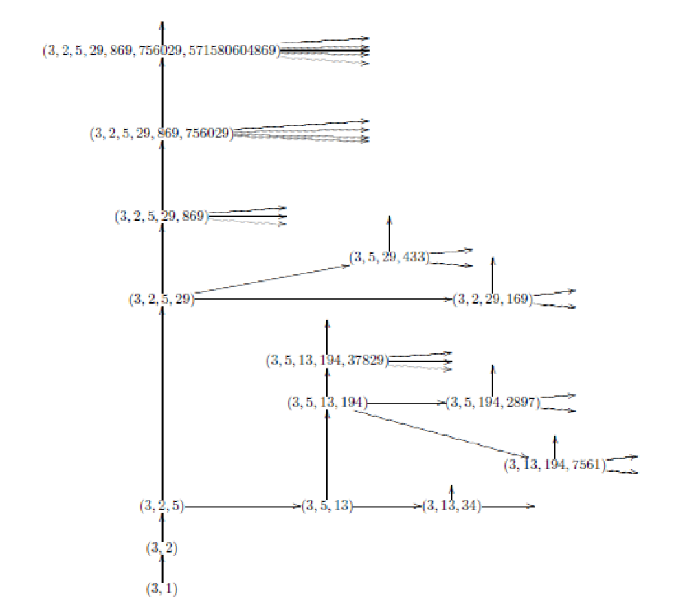
Figure 3 is the tree of castling transforms from a seed PV $(G\times GL(1),\rho\otimes\Lambda_{1},V(3)\otimes V(1))$ for 3-dimensional PV $(G,\rho,V(3)).$ Let $(G,\rho,V(3))$ be a 3-dimensional PV. In this section, we consider triples $(m_{1},m_{2},m_{3})$ in PV $(3,m_{1},m_{2},m_{3})$ which is castling transform of a $(3,1,1,2)=(G\times GL(1)\times GL(1)\times SL(2),\rho\otimes\Lambda_{1}\otimes\Lambda_{1}\otimes\Lambda_{1},V(3)\otimes V(1)\otimes V(1)\otimes V(2))$ . We explain that this triple $(m_{1},m_{2},m_{3})$ of integers satisfies a certain Diophantine equation. Here we remark that subtree of 4-simple prehomogeneous vector spaces in the tree of castling transforms of the seed prehomogeneous vector space $(G\times GL(1),\rho\otimes\Lambda_{1},V(3)\otimes V(1))$ . The branch $(3,2,5,29)$ , $(3,5,29,433)$ , $(3,2,29,169)$ , $(3,5,13,194)$ , $(3,5,194,2897)$ , $(3,13,194,7561)$ , $\dots$ satisfy the following relations:

$\begin{array}[]{l}2^{2}+5^{2}+29^{2}=870=3\times 2\times 5\times 29,\\ 5^{2}+29^{2}+433^{2}=188355=3\times 5\times 29\times 433,\\ 2^{2}+29^{2}+169^{2}=29406=3\times 2\times 29\times 169,\\ 5^{2}+13^{2}+194^{2}=37830=3\times 5\times 13\times 194,\\ 13^{2}+194^{2}+7561^{2}=57206526=3\times 13\times 194\times 7651,\\ \cdots\end{array}$

In general, the following theorem holds.

Theorem 3.3.

Let $(G,\rho,V(3))$ be a 3-dimensional PV. For 4-simple prehomogeneous vector space $(G\times GL(m_{1})\times SL(m_{2})\times SL(m_{3}),\rho\otimes\Lambda_{1}\otimes\Lambda_{1},V(3)\otimes V(m_{1})\otimes V(m_{2})\otimes V(m_{3}))$ (abbreviated by $(3,m_{1},m_{2},m_{3})$ ) in the tree of castling transforms with respect to the seed prehomogeneous vector space $(G\times GL(1),\rho\otimes\Lambda_{1},V(3)\otimes V(1))$ , the triple of integers $(m_{1},m_{2},m_{3})$ satisfies the relation $m_{1}^{2}+m_{2}^{2}+m_{3}^{2}=3m_{1}m_{2}m_{3}$ . Namely, $(m_{1},m_{2},m_{3})$ is a Markov triple.

Proof..

For 4-simple prehomogeneous vector space $(3,1,2,5)$ , the triplet of integers $(1,2,5)$ satisfies the relation $1^{2}+2^{2}+5^{2}=30=3\times 1\times 2\times 5$ . For 4-simple prehomogeneous vector space $(3,m_{1},m_{2},m_{3})$ ( $\mathrm{max}\{m_{1},m_{2}\}\leq m_{3}$ ) in the tree of castling transforms with respect to the seed prehomogeneous vector space $(G\times GL(1),\rho\otimes\Lambda_{1}V(3)\otimes V(1))$ , by castling transform, we get two 4-simple prehomogeneous vector spaces : $(3,m_{2},m_{3},3m_{2}m_{3}-m_{1}),(3,m_{1},m_{3},3m_{1}m_{3}-m_{2})$ , here we put $m^{\prime}:=3m_{2}m_{3}-m_{1},m^{\prime\prime}:=3m_{1}m_{3}-m_{2}$ . Then , if $(m_{1},m_{2},m_{3})$ satisfies a relation $m_{1}^{2}+m_{2}^{2}+m_{3}^{2}=3m_{1}m_{2}m_{3}$ , then $(m_{2},m_{3},m^{\prime})$ and $(m_{1},m_{3},m^{\prime\prime})$ also satisfy the relation $m_{2}^{2}+m_{3}^{2}+{m^{\prime}}^{2}=3m_{2}m_{3}m^{\prime}$ , $m_{1}^{2}+m_{3}^{2}+{m^{\prime\prime}}^{2}=3m_{1}m_{3}m^{\prime\prime}$ . In fact, $m_{2}^{2}+m_{3}^{2}+{m^{\prime}}^{2}$ $=m_{2}^{2}m_{3}^{2}+(3m_{2}m_{3}-m_{1})^{2}$ $=m_{2}^{2}m_{3}^{2}+9m_{2}^{2}m_{3}^{2}+m_{1}^{2}-6m_{1}m_{2}m_{3}=$ $(m_{1}^{2}m_{2}^{2}+m_{3}^{2})+9m_{2}^{2}m_{3}^{2}-6m_{1}m_{2}m_{3}$ $=3m_{1}m_{2}m_{3}+9m_{2}^{2}m_{3}^{2}-6m_{1}m_{2}m_{3}=3m_{2}m_{3}(3m_{2}m_{3}-m_{1})$ $=3m_{2}m_{3}m^{\prime}$ . This $(m_{1},m_{2},m_{3})$ is a Markov triple. ∎

3.3 Prehomogeneous vector spaces parametrized by a positive fraction smaller than 1

From the view point of classification of prehomogeneous , the following application is interesting.

Theorem 3.4.

We can make a prehomogeneous vector space of Markov type from any positive reduced fraction smaller than or equal to one. Conversely, any prehomogeneous vector space of Markov type comes from a reduced fraction smaller than or equal to 1.

Proof..

Form the one to one correspondence between Farey triple $(\frac{r}{s},\frac{r+r^{\prime}}{s+s^{\prime}},\frac{r^{\prime}}{s^{\prime}})$ in Farey tree and Christoffel $ab$ -word $(w(\frac{r}{s}),w(\frac{r}{s})w(\frac{r^{\prime}}{s^{\prime}}),w(\frac{r^{\prime}}{s^{\prime}}))$ in tree of Christoffel $ab$ -word in Figure 2 ( cf. [1]). Moreover there exists one to one correspondence between Markov triples and Christoffel $ab$ -words by Theorem 2.1. Thus we obtain the correspondence between triples in Farey tree and Markov triples. Since any positive fraction which is smaller than 1 or equal to 1 appear in second-entry in Farey triple in Farey tree and theorem 3.3, we have the correspondence between the set of positive fraction smaller than or equal to one and the set of prehomogeneous vector spaces of the form $(3,m_{1},m_{2},m_{3})=(G\times GL(m_{1})\times GL(m_{2})\times GL(m_{3}),\rho\otimes\Lambda_{1}\otimes\Lambda_{1}\otimes\Lambda_{1},V(3)\otimes V(m_{1})\otimes V(m_{2})\otimes V(m_{3}))$ . ∎

Here we introduce an example. A continued fraction is an expression obtained through an iterative process of representing a number as the sum of its integer part and the reciprocal of another number, then writing this other number as the sum of its integer part and another reciprocal, and so on.

Example 3.5.

We take a reduced fraction ${8\over{13}}$ . Since ${8\over{13}}=\displaystyle{\frac{1}{1+\frac{1}{1+\frac{1}{1+\frac{1}{1+\frac{1}{1+1}}}}}}=$ $[0;1,1,1,1,1+1]=[0;1,1,1,1,1,1]$ , ${8\over{13}}$ has neighbours $[0;1,1,1,1]={3\over 5}$ , $[0;1,1,1,1,1]={5\over 8}$ . Therefore ${8\over{13}}={3\over 5}\sharp{5\over 8}$ , where $\sharp$ means the Farey sum. Similarly, ${3\over 5}={1\over 2}\sharp{2\over 3}$ , ${5\over 8}={3\over 5}\sharp{2\over 3}={1\over 2}\sharp{2\over 3}\sharp{2\over 3}$ . Here we know, that a reduced fraction ${1\over p}$ (resp. ${{p-1}\over p}$ ) corresponds to Christoffel $ab$ -word $a^{p-1}b$ (resp. $ab^{p-1}$ ). Therefore ${3\over 5}$ , ${5\over 8}$ , ${8\over{13}}$ corresponds to $ab$ -word $abab^{2}$ , $abab^{2}ab^{2}$ , $abab^{2}abab^{2}ab^{2}$ respectively. Substituting matrices $A=\left(\begin{array}[]{cc}2&1\\ 1&1\end{array}\right),B=\left(\begin{array}[]{cc}5&2\\ 2&1\end{array}\right)$ to words $a,b$ , then we have associated matrices $C[{3\over 5}]:=ABAB^{2}=\left(\begin{array}[]{cc}1045&433\\ 613&254\end{array}\right),C[{5\over 8}]:=ABAB^{2}AB^{2}=\left(\begin{array}[]{cc}90927&37666\\ 53266&22071\end{array}\right),C[{8\over{13}}]:=ABAB^{2}ABAB^{2}AB^{2}=\left(\begin{array}[]{cc}118082927&48928105\\ \vskip 6.0pt plus 2.0pt minus 2.0pt\cr 69267835&28701388\end{array}\right)$ . We have a Markov triple $(433,37666,48928105)$ ( in fact $433^{2}+37666^{2}+48928105^{2}=3\times 433\times 37666\times 48928105$ ). Hence we have a prehomogeneous vector space $(SO(3)\times GL(433)\times GL(37666)\times GL(48928105),V(3)\otimes V(433)\otimes V(37666)\otimes V(48928105))$ as a castling transform of a seed prehomogeneous vector space $(SO(3)\times GL(1),V(3)\otimes V(1))$ .

3.4 Generalized cases

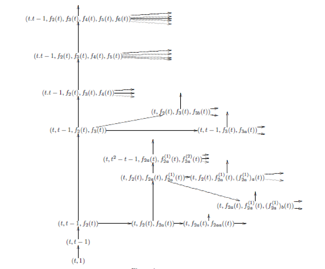
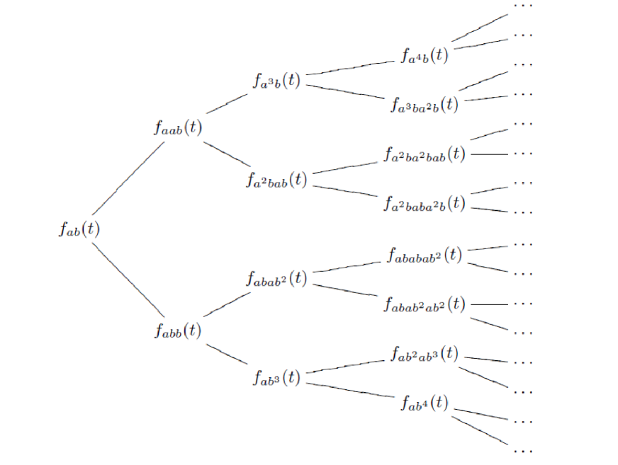
In this subsection, we generalize the three-dimensional prehomogeneous vector spaces we have dealt with so far to the t-dimensional prehomogeneous vector spaces. If we start from a prehomogeneous vector space with $t$ -dimensional representation space $V(t)$ , namely, $(GL(1)\times G,\Lambda_{1}\otimes\rho,V(1)\otimes V(t))$ , we have the following tree in Figure 4. of sequences of polynomials.

where

$f_{2}(t)=t^{2}-t-1$ ,

$f_{3}(t)=t^{4}-2t^{3}+t-1$ ,

$f_{4}(t)=t^{7}-3t^{6}+t^{5}+2t^{4}+t^{3}-t^{2}-t-1$ ,

$f_{5}(t)={t}^{14}-6\,{t}^{13}+11\,{t}^{12}-2\,{t}^{11}-9\,{t}^{10}-4\,{t}^{9}+10\,{t}^{8}+7\,{t}^{7}-2\,{t}^{6}-7\,{t}^{5}-3\,{t}^{4}+{t}^{3}+2\,{t}^{2}+t-1$ ,

$f_{6}(t)={t}^{28}-12\,{t}^{27}+58\,{t}^{26}-136\,{t}^{25}+127\,{t}^{24}+56\,{t}^{23}-126\,{t}^{22}-158\,{t}^{21}+229\,{t}^{20}+196\,{t}^{19}-158\,{t}^{18}-314\,{t}^{17}+34\,{t}^{16}+294\,{t}^{15}+146\,{t}^{14}-142\,{t}^{13}-213\,{t}^{12}-26\,{t}^{11}+116\,{t}^{10}+90\,{t}^{9}-9\,{t}^{8}-45\,{t}^{7}-23\,{t}^{6}+5\,{t}^{5}+9\,{t}^{4}+3\,{t}^{3}-{t}^{2}-t-1$ ,

$f_{3a}(t)=t^{5}-2t^{4}+2t+1,t^{5}-2t^{4}-t^{2}+2t+1$ ,

$f_{2a}^{(1)}(t)=t^{6}-2t^{5}-2t^{4}+4t^{3}-t^{2}-t-1$ ,

$(f_{2a}^{(1)})_{a}(t)=t^{9}-3t^{8}-t^{7}+8t^{6}-t^{5}-6t^{4}-2t^{3}+3t^{2}+3t-1$ ,

$(f_{2a}^{(1)})_{b}(t)=t^{10}-3t^{9}-2t^{8}+11t^{7}-t^{6}-12t^{5}+2t^{4}+3t^{2}+1$ ,

$f_{2a}^{(2)}(t)=t^{12}-4t^{11}+16t^{9}-10t^{8}-22t^{7}+15t^{6}+14t^{5}-5t^{4}-6t^{3}+t-1$ ,

$f_{3aa}(t)=t^{4}-t^{3}-3t^{2}+2t+1$ ,

This tree is very complicated. We can recognize this tree of Castling transform from a seed prehomogeneous vector space $(G\times GL(1),\rho\otimes\Lambda_{1},V(t)\otimes V(1))$ as following some ways. On this tree, there exist the following two kinds of operations:

$CT_{up}:(t,f_{1}(t),\dots,f_{l}(t))\mapsto(t,f_{1}(t),\dots,f_{l}(t),t\prod_{i=1}^{l}f_{i}(t)-1)$

(This operation corresponds to $\leftarrow$ in Figure 4).

$CT_{flat_{i}}:(t,f_{1}(t),\dots,f_{i-1},f_{i}(t),f_{i+1}(t),\dots,f_{r}(t))$

$\mapsto(t,f_{1}(t),\dots,f_{i-1},t\prod_{j=1,j\neq i}^{r}f_{j}(t)-f_{i}(t),f_{i+1}(t),\dots,f_{r}(t))$

(This operation corresponds to $\rightarrow$ in Figure 4).

We call the tree in Figure 4 $t$ -castling tree.

3.5 Castling Markov tree of $t$ -castling tree

In the tree in Figure 4, we choose ”4-simple-subtree” as follows:

Starting from

(t,f_{a}(t),f_{ab}(t),f_{b}(t)):=(t,t^{2}-t-1,t-1),

we consider subtree of the form

(t,f_{w(a,b)}(t),f_{w(a,b)w^{\prime}(a,b)}(t),f_{w^{\prime}(a,b)}(t))

that is parametrized by Christoffel $ab$ -word $w(a,b),w(a,b)w^{\prime}(a,b),$ $w(a,b)$ .

$CT_{flat_{b}}(t,f_{a}(t),f_{ab}(t),f_{b}(t))=(t,f_{a}(t),f_{ab}(t),tf_{a}(t)f_{ab}(t)-f_{b}(t))$ and we put

$f_{a^{2}b}(t):=tf_{a}(t)f_{ab}(t)-f_{b}(t)$

and we get a triplet $(f_{a}(t),f_{a^{2}b}(t),f_{ab}(t))$ that is parametrized by triple of Christoffel $ab$ -word $(a,a^{2}b,ab)$ .

$CT_{flat_{a}}(t,f_{a}(t),f_{ab}(t),f_{b}(t))=(t,tf_{ab}(t)f_{b}(t)-f_{a}(t),f_{ab}(t),f_{b}(t))$

and we put

$f_{ab^{2}}(t):=tf_{a}(t)f_{ab}(t)-f_{b}(t)$

and we get a triplet $(f_{a}(t),f_{ab^{2}}(t),f_{ab}(t))$ that is parametrized by triple of Christoffel $ab$ -word $(ab,ab^{2},b)$ . In general, we get

(f_{w(a,b)}(t),f_{w(a,b)^{2}w^{\prime}(a,b)}(t),f_{w(a,b)w^{\prime}(a,b)}(t))

and

(f_{w(a,b)w^{\prime}(a,b)}(t),f_{w(a,b)w^{\prime}(a,b)^{2}}(t),f_{w^{\prime}(a,b)}(t))

as follows:

$CT_{flat_{w^{\prime}(a,b)}}(t,f_{w(a,b)}(t),f_{w(a,b)w^{\prime}(a,b)}(t),f_{w^{\prime}(a,b)}(t))$

$=(t,f_{w(a,b)}(t),f_{w(a,b)w^{\prime}(a,b)}(t),tf_{w(a,b)}(t)f_{w(a,b)w^{\prime}(a,b)}(t)-f_{w^{\prime}(a,b)}(t))$

and we put $f_{w(a,b)^{2}w^{\prime}(a,b)}(t)=tf_{w(a,b)}(t)f_{w(a,b)w^{\prime}(a,b)}(t)-f_{w^{\prime}(a,b)}(t)$ and get a triple

(f_{w(a,b)}(t),f_{w(a,b)^{2}w^{\prime}(a,b)}(t),f_{w(a,b)w^{\prime}(a,b)}(t)).

$CT_{flat_{w(a,b)}}(t,f_{w(a,b)}(t),f_{w(a,b)w^{\prime}(a,b)}(t),f_{w^{\prime}(a,b)}(t))=(t,tf_{w(a,b)}(t)f_{w(a,b)w^{\prime}(a,b)}(t)-f_{w^{\prime}(a,b)}(t),f_{w(a,b)w^{\prime}(a,b)}(t),$ $f_{w^{\prime}(a,b)}(t))$

and we put $f_{w(a,b)w^{\prime}(a,b)^{2}}(t)=tf_{w(a,b)w^{\prime}(a,b)}(t)f_{w^{\prime}(a,b)}(t)-f_{w(a,b)}(t)$ and get a triple

(f_{w(a,b)w^{\prime}(a,b)}(t),f_{w(a,b)w^{\prime}(a,b)^{2}}(t),f_{w^{\prime}(a,b)}(t)).

Thus we have a class $\{(f_{w(a,b)}(t),f_{w(a,b)w^{\prime}(a,b)}(t),f_{w^{\prime}(a,b)}(t))\}_{(w(a,b),w(a,b)w^{\prime}(a,b),w^{\prime}(a,b))\textrm{is a triple of Christoffel words}}$ and tree Figure 5 of them.

If we substitute $t=3$ , we have the tree of Markov triples. Here we call these polynomials castling-Markov polynomials and call subtree

$\{(f_{w(a,b)}(t),f_{w(a,b)w^{\prime}(a,b)}(t),f_{w^{\prime}(a,b)}(t))\}_{(w(a,b),w(a,b)w^{\prime}(a,b),w^{\prime}(a,b))\textrm{is a triple of Christoffel words}}$ Castling Markov tree. In specially, subtree of subsequence $\{f_{a^{n}b}(t)\}$ satisfies the following recurrence relation:

f_{a^{n+2}b}(t)=tf_{a^{n+1}b}(t)-f_{a^{n}b}(t).

(3.1)

Furthermore we have the following theorem.

Theorem 3.6.

For a Christoffel $ab$ -word triple $(w,ww^{\prime},w^{\prime})$ where $ww^{\prime}$ means a word that connects $w^{\prime}$ after $w$ , let $(f_{w}(t),f_{ww^{\prime}}(t),f_{w^{\prime}}(t))$ be triplet of castling Markov polynomials corresponding to $(w,ww^{\prime},w^{\prime})$ . Then $(f_{w}(t),f_{ww^{\prime}}(t),f_{w^{\prime}}(t))$ is a solution of modified Markov equation

x^{2}+y^{2}+z^{2}+(t-3)=txyz.

(3.2)

Proof..

For a $t$ -deformation $(a_{t},b_{t},c_{t}):=(f_{w(a,b)}(t),f_{w(a,b)w^{\prime}(a,b)}(t),f_{w^{\prime}(a,b)})$ of a Markov triple $(a,b,c)=(\mathrm{Tr}w(A,B)/3,\mathrm{Tr}w(A,B)w^{\prime}(A,B)/3,\mathrm{Tr}w^{\prime}(A,B)/3)$ , let two triples that come from $(a_{t},b_{t},c_{t})$ via castling transforms:

\left\{\begin{array}[]{l}(a_{t},\tilde{c}_{t},b_{t})=(f_{w(a,b)}(t),f_{w(a,b)^{2}w^{\prime}(a,b)}(t),f_{w(a,b)w^{\prime}(a,b)}(t))=(a_{t},ta_{t}b_{t}-c_{t},b_{t})\\ (b_{t},\tilde{a}_{t},c_{t})=(f_{w(a,b)w^{\prime}(a,b)}(t),f_{w(a,b)w^{\prime}(a,b)^{2}}(t),f_{{w^{\prime}(a,b)}(t)})=(b_{t},tb_{t}c_{t}-a_{t},c_{t})\end{array}\right.

(3.3)

Then, since $a_{t}^{2}+b_{t}^{2}+c_{t}^{2}+(t-3)$ $=ta_{t}b_{t}c_{t}$ ,

$a_{t}^{2}+\tilde{c}_{t}^{2}+b^{2}_{t}+(t-3)$ $=a_{t}^{2}+(ta_{t}b_{t}-c_{t})^{2}+(t-3)=t^{2}a_{t}^{2}b_{t}^{2}-ta_{t}b_{t}c_{t}$ $=ta_{t}(ta_{t}b_{t}-c_{t})b_{t}$ $=ta_{t}\tilde{c}_{t}b_{t}$ ,

$b_{t}^{2}+\tilde{a}_{t}^{2}+c^{2}_{t}+(t-3)$ $=b_{t}^{2}+(tb_{t}c_{t}-a_{t})^{2}+(t-3)$ $=t^{2}b_{t}^{2}c_{t}^{2}-ta_{t}b_{t}c_{t}=b_{t}(tb_{t}c_{t}-a_{t})c_{t}$ $=tb_{t}\tilde{a}_{t}c_{t}$ . Therefore $(a_{t},\tilde{c}_{t},b_{t})$ and $(b_{t},\tilde{a}_{t},c_{t})$ are also solutions of $t$ -Markov equation $x^{2}+y^{2}+z^{2}+(t-3)=txyz$ .

∎

3.6 Chebyshev polynomials and castling Markov polynomials

The Chebyshev polynomials of the first kind are defined by the recurrence relation $T_{0}(x)=1,T_{1}(x)=x,T_{n+1}(x)=2xT_{n}(x)-T_{n-1}(x)$ . The Chebyshev polynomials of the second kind are defined by the recurrence relation $U_{0}(x)=1,U_{1}(x)=2x,U_{n+1}(x)=2xU_{n}(x)-U_{n-1}(x)$ . Modified Chebyshev polynomials of the first (resp. second) kind are defined by $t_{n}(x):=2T_{n}({x\over 2})$ (resp. $u_{n}(x):=U_{n}({x\over 2})).$ From the property of Chebyshev polynomials, We obtain the following result.

Proposition 3.7.

Here if we put $S_{n}(t):=f_{a^{n-1}b}(t)$ and $S_{0}(t):=1,S_{1}(t)=t-1$ , we obtain the following:

(1)

\begin{array}[]{cc}S_{n}(t)=\displaystyle{{1\over{\sqrt{t^{2}-4}}}}&\biggl{[}\displaystyle{(t-1)\left\{\left({{t+\sqrt{t^{2}-4}}\over 2}\right)^{n}-\left({{t-\sqrt{t^{2}-4}}\over 2}\right)^{n}\right\}}\\ &\displaystyle{-\left\{\left({{t+\sqrt{t^{2}-4}}\over 2}\right)^{n-1}-\left({{t-\sqrt{t^{2}-4}}\over 2}\right)^{n-1}\right\}}\biggr{]}\end{array}

(3.4)

(2)

S_{n}(t)=tu_{n}(t)-u_{n-1}(t),

(3.5)

where $u_{n}(t)$ is a Chebyshev polynomial of second type.

(3)

S_{n}(t):=\det\left(\begin{array}[]{ccccc}t-1&1&0&\cdots&0\\ 1&t&1&&\vdots\\ 0&1&\ddots&\ddots&0\\ \vdots&\ddots&\ddots&t&1\\ 0&\cdots&0&1&t\end{array}\right)~{}~{}(n\geq 1)

(3.6)

Furthermore we see the following property on the sub-sequences $\{f_{ab^{n}}(t)\}$ .

Remark 3.8.

$f_{ab^{n}}(t)$ can be written by modified Chebyshev polynomials of first and second kind as follows:

f_{ab^{n}}(t)=({1\over 2})t_{n}(t^{2}-t)+({1\over 2})(t^{2}-t-2)u_{n-1}(t^{2}-t)=T_{n}({1\over 2}t(t-1))+({1\over 2})(t^{2}-t-2)U_{n-1}({1\over 2}t(t-1)).

(3.7)

If we put

\left\{\begin{array}[]{c}p_{n}(t)={1\over 2}t_{n}(t^{2}-t)+{1\over 2}(t^{2}-t-2)u_{n-1}(t^{2}-t)\\ q_{n}(t)={1\over 2}t_{n}(t^{2}-t)+{1\over 2}(t^{2}-t+2)u_{n-1}(t^{2}-t)\end{array}\right.

(3.8)

from properties of modified Chebyshev polynomials, we obtain

\left\{\begin{array}[]{c}t_{n+2}(t)-t_{n}(t)=(t^{4}-4)u_{n}(t)\\ u_{n+2}(t)-u_{n}(t)=t_{n+2}(t)\end{array}\right..

(3.9)

Thus

\left\{\begin{array}[]{c}p_{n+2}(t)-p_{n}(t)=(t^{2}-t-2)q_{n+1}(t)\\ q_{n+2}(t)-q_{n}(t)=(t^{2}-t+2)p_{n+1}(t)\end{array}\right.

(3.10)

hold.

For $f_{a^{n-1}b}(t)=u_{n+1}(t)-u_{n}(t)$ , $f_{a^{n}b}(t)-f_{a^{n-1}b}(t)=t_{n+1}(t)$ . If we put $g_{n}(t)=t_{n+1}(t)-t_{n}(t)$ , we have the following relation : $g_{n+2}(t)-g_{n}(t)=(t^{4}-4)(u_{n-1}(t)-u_{n-2}(t))=(t^{2}-4)f_{a^{n-3}b}(t)$ .

6.4. Continued fraction of polynomials and castling Markov polynomials

We observe that castling-Markov polynomials are related to continued fraction of polynomials. For example,

$\displaystyle{\frac{f_{a^{3}ba^{3}ba^{2}b}(t)}{f_{a^{3}ba^{3}ba^{3}ba^{2}b}(t)}}$

$=\displaystyle{\frac{1}{{t}^{5}-{t}^{4}-3\,{t}^{3}+2\,{t}^{2}+t+\frac{1}{-({t}^{5}-{t}^{4}-3\,{t}^{3}+2\,{t}^{2}+t)+\frac{1}{-({t}^{3}-{t}^{2}-2\,t+1)}}}}$

$=[0,{t}^{5}-{t}^{4}-3\,{t}^{3}+2\,{t}^{2}+t,-{t}^{5}+{t}^{4}+3\,{t}^{3}-2\,{t}^{2}-t,{t}^{5}-{t}^{4}-3\,{t}^{3}+2\,{t}^{2}+t,-{t}^{3}+{t}^{2}+2\,t-1],$

$=[0;tf_{a^{3}b}(t),-tf_{a^{3}b}(t),tf_{a^{3}b}(t),-f_{a^{2}b}(t)]$

$\displaystyle{\frac{f_{a^{2}ba^{2}bab}(t)}{f_{a^{2}ba^{2}baba^{2}bab}(t)}=[0;tf_{a^{2}b}(t),-tf_{a^{2}bab}(t),t,-t,f_{b}(t)]},$

$\displaystyle{\frac{f_{a^{2}ba^{2}baba^{2}bab}(t)}{f_{a^{2}baba^{2}ba^{2}baba^{2}bab}(t)}=[0;tf_{a^{2}bab}(t),-tf_{a^{2}b}(t),tf_{a^{2}bab}(t),-t,t,-f_{b}(t)]},$

$\displaystyle{\frac{f_{a^{2}babab}(t)}{f_{a2baba2babab}(t)}=[0;tf_{a^{2}bab}(t),-tf_{a^{2}bab}(t),-t,f_{b}(t)]},$

$\displaystyle{\frac{f_{a^{2}baba^{2}babab}(t)}{f_{a2baba2baba2babab}(t)}=[0;tf_{a^{2}bab}(t),-tf_{a^{2}bab}(t),tf_{a^{2}bab}(t),t,-f_{b}(t)]},$

$\displaystyle{\frac{f_{ababab^{2}}(t)}{f_{ababab^{2}abab^{2}}(t)}=[0;tf_{abab^{2}}(t),-tf_{abab^{2}}(t),f_{ab}(t),-f_{ab}(t)]},$

$\displaystyle{\frac{f_{ababab^{2}abab^{2}}(t)}{f_{ababab^{2}abab^{2}abab^{2}}(t)}=[0;tf_{abab^{2}}(t),-tf_{abab^{2}}(t),tf_{abab^{2}}(t),-f_{ab}(t),f_{ab}(t)]},$

$\begin{array}[]{l}\displaystyle{\frac{f_{abab^{2}abab^{2}ab^{2}}(t)}{f_{abab^{2}abab^{2}abab^{2}ab^{2}}(t)}=[0;tf_{abab^{2}}(t),-tf_{abab^{2}}(t),tf_{b}(t),-f_{ab}(t)]},\\ \displaystyle{\frac{f_{ab^{2}ab^{3}}(t)}{f_{ab^{2}ab^{3}ab^{3}}(t)}=[0;tf_{ab^{3}}(t),-tf_{ab^{3}}(t),f_{a^{2}b}(t),-f_{b}(t)]},\\ \displaystyle{\frac{f_{ab^{2}ab^{3}ab^{3}}(t)}{f_{ab^{2}ab^{3}ab^{3}ab^{3}}(t)}=[0;tf_{ab^{2}}(t),-tf_{ab^{2}}(t),tf_{ab^{2}}(t),-f_{ab^{2}}(t),-f_{a^{2}b}(t),f_{b}(t)]},\\ \displaystyle{\frac{f_{ab^{4}}(t)}{f_{ab^{3}ab^{4}}(t)}=[0;tf_{ab^{3}}(t),-f_{ab^{2}}(t),-f_{ab}(t),f_{ab^{2}}(t)]}.\end{array}$

4 A relation between $q$ -deformations and $t$ -deformations

In this section, we introduce a relation between $q$ -deformation of Markov triples and $t$ -deformation of ones. $\mathrm{lim}_{q\mapsto 1}h_{w(a,b)}(q)=\frac{1}{3}\mathrm{Tr}(w(A,B))=\mathrm{lim}_{t\mapsto 3}f_{w}(t)$ where $\frac{1}{3}\mathrm{Tr}(w(A,B))$ is a Markov number corresponding to Christoffel $ab$ -word $w(a,b)$ . Here we list up $q$ -deformations and $t$ -deformations as follows:

(i) List of $q$ -deformations $\{h_{w(a,b)}(q)\}_{q}$

$h_{a}(q)=\frac{1}{q},$

$h_{b}(q)=q^{-2}(q^{2}+1)$

$h_{ab}(q)=q^{-3}({q}^{4}+{q}^{3}+{q}^{2}+q+1),$

$h_{a^{2}b}(q)=q^{-4}({q}^{6}+2\,{q}^{5}+2\,{q}^{4}+3\,{q}^{3}+2\,{q}^{2}+2\,q+1)$

$h_{ab^{2}}(q)=q^{-5}({q}^{8}+2\,{q}^{7}+4\,{q}^{6}+5\,{q}^{5}+5\,{q}^{4}+5\,{q}^{3}+4\,{q}^{2}+2\,q+1)$

$h_{a^{3}b}(q)=q^{-5}({q}^{8}+3\,{q}^{7}+4\,{q}^{6}+6\,{q}^{5}+6\,{q}^{4}+6\,{q}^{3}+4\,{q}^{2}+3\,q+1),$

$h_{a^{2}bab}(q)=q^{-7}({q}^{12}+4\,{q}^{11}+9\,{q}^{10}+16\,{q}^{9}+23\,{q}^{8}+29\,{q}^{7}+30\,{q}^{6}+29\,{q}^{5}+23\,{q}^{4}+16\,{q}^{3}+9\,{q}^{2}+4\,q+1),$

$h_{abab^{2}}(q)=q^{-8}({q}^{14}+4\,{q}^{13}+11\,{q}^{12}+22\,{q}^{11}+36\,{q}^{10}+50\,{q}^{9}+60\,{q}^{8}+65\,{q}^{7}+60\,{q}^{6}+50\,{q}^{5}+36\,{q}^{4}+22\,{q}^{3}+11\,{q}^{2}+4\,q+1),$

$h_{ab^{3}}(q)=q^{-7}({q}^{12}+3\,{q}^{11}+8\,{q}^{10}+14\,{q}^{9}+20\,{q}^{8}+25\,{q}^{7}+27\,{q}^{6}+25\,{q}^{5}+20\,{q}^{4}+14\,{q}^{3}+8\,{q}^{2}+3\,q+1),$

$h_{a^{4}b}(q)=q^{-9}({q}^{16}+4\,{q}^{15}+13\,{q}^{14}+29\,{q}^{13}+53\,{q}^{12}+82\,{q}^{11}+110\,{q}^{10}+131\,{q}^{9}+139\,{q}^{8}+131\,{q}^{7}+110\,{q}^{6}+82\,{q}^{5}+53\,{q}^{4}+29\,{q}^{3}+13\,{q}^{2}+4\,q+1),$

$h_{a^{3}ba^{2}b}(q)=q^{-9}({q}^{16}+6\,{q}^{15}+18\,{q}^{14}+40\,{q}^{13}+72\,{q}^{12}+110\,{q}^{11}+148\,{q}^{10}+175\,{q}^{9}+185\,{q}^{8}+175\,{q}^{7}+148\,{q}^{6}+110\,{q}^{5}+72\,{q}^{4}+40\,{q}^{3}+18\,{q}^{2}+6\,q+1),$

$h_{a^{2}ba^{2}bab}(q)=q^{-11}({q}^{20}+7\,{q}^{19}+26\,{q}^{18}+70\,{q}^{17}+151\,{q}^{16}+276\,{q}^{15}+440\,{q}^{14}+623\,{q}^{13}+793\,{q}^{12}+914\,{q}^{11}+959\,{q}^{10}+914\,{q}^{9}+793\,{q}^{8}+623\,{q}^{7}+440\,{q}^{6}+276\,{q}^{5}+151\,{q}^{4}+70\,{q}^{3}+26\,{q}^{2}+7\,q+1),$

$h_{a^{2}babab}(q)=q^{-10}({q}^{18}+6\,{q}^{17}+20\,{q}^{16}+49\,{q}^{15}+97\,{q}^{14}+164\,{q}^{13}+240\,{q}^{12}+313\,{q}^{11}+366\,{q}^{10}+385\,{q}^{9}+366\,{q}^{8}+313\,{q}^{7}+240\,{q}^{6}+164\,{q}^{5}+97\,{q}^{4}+49\,{q}^{3}+20\,{q}^{2}+6\,q+1),$

$h_{ababab^{2}}(q)=q^{-11}({q}^{20}+6\,{q}^{19}+22\,{q}^{18}+59\,{q}^{17}+128\,{q}^{16}+235\,{q}^{15}+375\,{q}^{14}+533\,{q}^{13}+679\,{q}^{12}+784\,{q}^{11}+822\,{q}^{10}+784\,{q}^{9}+679\,{q}^{8}+533\,{q}^{7}+375\,{q}^{6}+235\,{q}^{5}+128\,{q}^{4}+59\,{q}^{3}+22\,{q}^{2}+6\,q+1),$

$h_{abab^{2}ab^{2}}(q)=q^{-13}({q}^{24}+7\,{q}^{23}+30\,{q}^{22}+94\,{q}^{21}+237\,{q}^{20}+504\,{q}^{19}+932\,{q}^{18}+1531\,{q}^{17}+2264\,{q}^{16}+3045\,{q}^{15}+3746\,{q}^{14}+4236\,{q}^{13}+4412\,{q}^{12}+4236\,{q}^{11}+3746\,{q}^{10}+3045\,{q}^{9}+2264\,{q}^{8}+1531\,{q}^{7}+932\,{q}^{6}+504\,{q}^{5}+237\,{q}^{4}+94\,{q}^{3}+30\,{q}^{2}+7\,q+1),$

$h_{ab^{2}ab^{3}}(q)=q^{-12}({q}^{22}+6\,{q}^{21}+24\,{q}^{20}+70\,{q}^{19}+165\,{q}^{18}+328\,{q}^{17}+567\,{q}^{16}+870\,{q}^{15}+1201\,{q}^{14}+1504\,{q}^{13}+1717\,{q}^{12}+1795\,{q}^{11}+1717\,{q}^{10}+1504\,{q}^{9}+1201\,{q}^{8}+870\,{q}^{7}+567\,{q}^{6}+328\,{q}^{5}+165\,{q}^{4}+70\,{q}^{3}+24\,{q}^{2}+6\,q+1),$

$h_{ab^{4}}(q)=q^{-9}({q}^{16}+4\,{q}^{15}+13\,{q}^{14}+29\,{q}^{13}+53\,{q}^{12}+82\,{q}^{11}+110\,{q}^{10}+131\,{q}^{9}+139\,{q}^{8}+131\,{q}^{7}+110\,{q}^{6}+82\,{q}^{5}+53\,{q}^{4}+29\,{q}^{3}+13\,{q}^{2}+4\,q+1),$

(ii) List of $t$ -deformations $\{f_{w(a,b)}(t)\}_{t}$

$\begin{array}[]{l}f_{a}(t)=1,\\ f_{b}(t)=t-1,\\ f_{ab}(t)=t^{2}-t-1,\\ f_{a^{2}b}(t)=t^{3}-t^{2}-2t+1,\\ f_{ab^{2}}(t)=t^{4}-2t^{3}+t-1,\\ f_{a^{3}b}(t)=t^{4}-t^{3}-3t^{2}+2t+1,\\ f_{a^{2}bab}(t)=t^{6}-2t^{5}-2t^{4}+4t^{3}+t^{2}-t-1,\\ f_{abab^{2}}(t)=t^{7}-3t^{6}+t^{5}+3t^{4}-2t^{3}+1,\\ f_{ab^{3}}(t)=t^{6}-3t^{5}+2t^{4}+t^{3}-3t^{2}+2t+1,\\ f_{a^{4}b}(t)=t^{5}-t^{4}-4t^{3}+3t^{2}+3t-1,\\ f_{a^{3}ba^{2}b}(t)=t^{8}-2t^{7}-4t^{6}+8t^{5}+4t^{4}-8t^{3}+t-1,\\ f_{a^{2}ba^{2}bab}(t)=t^{10}-3t^{9}-2t^{8}+11t^{7}-t^{6}-12t^{5}+2t^{4}+4t^{3}+1,\\ f_{a^{2}babab}(t)=t^{9}-3t^{8}-t^{7}+8t^{6}-t^{5}-6t^{4}-2t^{3}+3t^{2}+3t-1,\\ f_{ababab^{2}}(t)=t^{10}-4t^{9}+3t^{8}+5t^{7}-6t^{6}-t^{5}+t^{4}+3t^{3}-t^{2}-2t+1,\\ f_{abab^{2}ab^{2}}(t)=t^{12}-5t^{11}+7t^{10}+2t^{9}-12t^{8}+8t^{7}+2t^{6}-4t^{5}+1,\\ f_{ab^{2}ab^{3}}(t)=t^{11}-5t^{10}+8t^{9}-2t^{8}-9t^{7}+13t^{6}-4t^{5}-6t^{4}+5t^{3}-t^{2}-2t+1,\\ f_{ab^{4}}(t)=t^{8}-4t^{7}+5t^{6}-t^{5}-5t^{4}+7t^{3}-t^{2}-2t+1,\end{array}$

Theorem 4.1.

(i)For Christoffel $ab$ -word $w$ , let $f_{w}(t)$ be $t$ -deformation of Markov number corresponding to $w$ and $h_{w}(q)$ be $q$ -deformation of Markov number corresponding to $w$ .

Then the following relation holds:

f_{w}([3]_{q}/q)=qh_{w}(q).

(4.1)

(ii) A set of $q$ -deformations and a set of $t$ -deformations have a one to one correspondence.

Proof..

(i) From Theorem 2.5 and the construction of $(f_{w}(t),f_{ww^{\prime}}(t),f_{w^{\prime}}(t))$ and $(h_{w}(q),h_{ww^{\prime}}(q),h_{w^{\prime}}(q))$ , we obtain $f([q^{-1}[3]_{q})=qh_{w}(q)$ .

(ii)Let $(x,y,z)=(f_{w}(t),f_{ww^{\prime}}(t),f_{w^{\prime}}(t)$ be a solution of $x^{2}+y^{2}+z^{2}+(t-3)=txyz.$ Then put $t=q^{-1}[3]_{q}$ and deform the equation as follows: $x^{2}+y^{2}+z^{2}+\frac{[3]_{q}-3q}{q}=q^{-1}[3]_{q}xyz\Leftrightarrow(x,y,z)=(q\tilde{x},q\tilde{y},q\tilde{z}),~{}~{}(q\tilde{x})^{2}+(q\tilde{y})^{2}+(q\tilde{z})^{2}=q^{-1}[3]_{q}(q\tilde{x})(q\tilde{y})(q\tilde{z})\Leftrightarrow q^{2}\{\tilde{x}^{2}+\tilde{y}^{2}+\tilde{z}^{2}\}=q^{2}[3]_{q}\tilde{x}\tilde{y}\tilde{z}\Leftrightarrow\tilde{x}^{2}+\tilde{y}^{2}+\tilde{z}^{2}=[3]_{q}\tilde{x}\tilde{y}\tilde{z}.$ Here from (i) $f_{w}(q^{-1}[3]_{q})=qh_{w}(q)$ , we have

$(qh_{w}(q))^{2}+(qh_{ww^{\prime}}(q))^{2}+(qh_{w^{\prime}}(q))^{2}+\frac{(1-q)^{2}}{q^{3}}=q^{-1}[3]_{q}(qh_{w}(q))(qh_{ww^{\prime}}(q))(qh_{w^{\prime}}(q)).$

This means that $(x,y,z)=(h_{w}(q),h_{ww^{\prime}}(q),h_{w^{\prime}}(q))$ is a solution of $x^{2}+y^{2}+z^{2}+\frac{(1-q)^{2}}{q^{3}}=[3]_{q}xyz$ .

On the other hand, let $(x,y,z)=(h_{w}(q),h_{ww^{\prime}}(q),h_{w^{\prime}}(q))$ be a solution of $x^{2}+y^{2}+z^{2}+\frac{(1-q)^{2}}{q^{3}}=[3]_{q}xyz.$ Since $\frac{(q-1)^{2}}{q^{3}}=\frac{q^{-1}[3]_{q}-3}{q^{2}}$ and (i) $f_{w}(q^{-1}[3]_{q})=qh_{w}(q)$ ,

$(qh_{w}(q))^{2}+(qh_{ww^{\prime}}(q))^{2}+(qh_{w^{\prime}}(q))^{2}+(q^{-1}[3]_{q}-3)=q^{-1}[3]_{q}(qh_{w}(q))(qh_{ww^{\prime}}(q))(qh_{w^{\prime}}(q))$

$\Leftrightarrow$

$f_{w}(t)^{2}+f_{ww^{\prime}}(t)^{2}+f_{w^{\prime}}(t)^{2}+(t-3)=tf_{w}(t)f_{ww^{\prime}}(t)f_{w^{\prime}}(t).$

This means that $(x,y,z)=(f_{w}(t),f_{ww^{\prime}}(t),f_{w^{\prime}}(t))$ is a solution of $x^{2}+y^{2}+z^{2}+(t-3)=txyz$ . ∎

Example 4.2.

(i) $f_{a^{2}b}(q^{-1}[3]_{q})=q^{-3}[3]_{q}^{3}-q^{-2}[3]_{q}^{2}-2q^{-1}[3]_{q}+1$

$=q^{-3}\{q^{6}+2q^{5}+2q^{4}+3q^{3}+2q^{2}+2q+1\}$

$=qh_{a^{2}b}(q)$

(ii) $qh_{a^{2}bab}(q)=q^{-6}(q^{12}+4q^{11}+9q^{10}+16q^{9}+23q^{8}+29q^{7}+30q^{6}+29q^{5}+23q^{4}+16q^{3}+9q^{2}+4q+1)$

$=(q^{-1}[3]_{q})^{6}-2(q^{-1}[3]_{q})^{5}-2(q^{-1}[3]_{q})^{4}+4(q^{-1}[3]_{q})^{3}+(q^{-1}[3]_{q})^{2}-(q^{-1}[3]_{q})-1$

$=t^{6}-2t^{5}-2t^{4}+4t^{3}+t^{2}-t-1$

$=f_{a^{2}bab}(t).$

Problem

(1) In classical theory, a Markov triple gives the best approximation of a quadratic irrational to rational. Can $q$ -deformations also say something about $q$ -quadratic irrational number?

(2) There is a relation between $q$ -deformations and $t$ -deformations, then is there a deep relation between quantum topology , analytic number theory and prehomogeneous vector spaces?

References

[1] M .Aigner, Markov’s theorem and 100 years of the uniqueness conjecture. A mathematical journey from irrational numbers to perfect matchings. Springer, Cham, 2013. x+257 pp. ISBN: 978-3-319-00887-5; 978-3-319-00888-2
[2] E. Bombieri, Continued fractions and the Markoff tree. Expositiones Mathematicae 25(3) (2007), 187–213.
[3] H. Cohn, Minimal geodesics on Fricke’s torus-covering. In: Proceedings of the Conference on Riemann Surfaces and Related Topics (Stony Brook, 1978, I. Kra and B. Maskit, eds.), Ann. Math. Studies 97, Princeton Univ. Press (1981),
[4] H. Cohn, Markoff forms and primitive words. Mathematische Annalen 196 (1972), 8–22.
[5] S. Morier-Genoud and V. Ovsienko, $q$ -Deformed rationals and $q$ -continued fractions, Forum Math. Sigma 8 (2020), e13, 55 pp.
[6] M.Sato and T.Kimura A classification of irreducible prehomogeneous vector spaces and their relative invariants.Nagoya Math. J. 65 (1977), 1 - 155.
[7] T.Kimura, Introduction to prehomogeneous vector spaces. American Mathematical Society, Providence, RI, 2003. xxii+288 pp. ISBN: 0-8218-2767-7.

qq-Deformations and tt-Deformations of the Markov triples

Abstract

Introduction

1 qq-Deformation of continued fractions due to Morier-Genoud and Ovsienko

Theorem 1.1.

Example 1.2.

Theorem 1.3.

Theorem 1.4.

2 qq-Deformations of the Markov equation and Markov triples

Theorem 2.1.

Lemma 2.2.

Proof..

Lemma 2.3.

Theorem 2.4.

Proof..

Remark 2.5.

Theorem 2.6.

Proof..

Remark 2.7.

Example 2.8.

2.1 An application of qq-Markov triples to fixed points of associated Cohn matrices

Theorem 2.9.

Proof..

Example 2.10.

Remark 2.11.

Remark 2.12.

2.2 Other qq-deformations of Markov triples

Proposition 2.13.

Proposition 2.14.

Example 2.15.

Example 2.16.

3 A relation of castling transformations of 3-dimensional prehomogeneous vector spaces and Markov triplets and the generalization

3.1 Prehomogeneous vector spaces and castling transformations

Example 3.1.

Remark 3.2.

3.2 A relation between castling transformations of 3-dimensional prehomogeneous vector spaces and Markov triples

Theorem 3.3.

Proof..

3.3 Prehomogeneous vector spaces parametrized by a positive fraction smaller than 1

Theorem 3.4.

Proof..

Example 3.5.

3.4 Generalized cases

3.5 Castling Markov tree of tt-castling tree

Theorem 3.6.

Proof..

3.6 Chebyshev polynomials and castling Markov polynomials

Proposition 3.7.

Remark 3.8.

4 A relation between qq-deformations and tt-deformations

Theorem 4.1.

Proof..

Example 4.2.

References

$q$ -Deformations and $t$ -Deformations of the Markov triples

1 $q$ -Deformation of continued fractions due to Morier-Genoud and Ovsienko

2 $q$ -Deformations of the Markov equation and Markov triples

2.1 An application of $q$ -Markov triples to fixed points of associated Cohn matrices

2.2 Other $q$ -deformations of Markov triples

3.5 Castling Markov tree of $t$ -castling tree

4 A relation between $q$ -deformations and $t$ -deformations