Quadratic and Cubic Regularisation Methods with Inexact function and Random Derivatives for Finite-Sum Minimisation
Abstract
This paper focuses on regularisation methods using models up to the third order to search for up to second-order critical points of a finite-sum minimisation problem. The variant presented belongs to the framework of [3]: it employs random models with accuracy guaranteed with a sufficiently large prefixed probability and deterministic inexact function evaluations within a prescribed level of accuracy. Without assuming unbiased estimators, the expected number of iterations is or when searching for a first-order critical point using a second or third order model, respectively, and of when seeking for second-order critical points with a third order model, in which , , is the th-order tolerance. These results match the worst-case optimal complexity for the deterministic counterpart of the method. Preliminary numerical tests for first-order optimality in the context of nonconvex binary classification in imaging, with and without Artifical Neural Networks (ANNs), are presented and discussed.
Index Terms:
evaluation complexity, regularization methods, inexact functions and derivatives, stochastic analysisI Introduction
We consider adaptive regularisation methods to compute an approximate -th order, , local minimum of the finite-sum minimisation problem
| (1) |
where , .
Problem (1) has recently received a large attention since it includes a variety of applications, such as least-squares approximation and Machine Learning, and covers optimization problems in imaging. In fact, Convolutional Neural Networks (CNNs) have been successfully employed for classification in imaging and for recovering an image from a set of noisy measurements, and compares favourably with well accessed iterative reconstruction methods combined with suitable regularization. Investigating the link between traditional approaches and CNNs is an active area of research as well as the efficient solution of nonconvex optimization problems which arise from training the networks on large databases of images and can be cast in the form (1) with being a large positive integer (see e.g., [2, 9, 28, 31, 39]).
The wide range of methods used in literature to solve (1) can be classified as first-order methods, requiring only the gradient of the objective and second-order procedures, where the Hessian is also needed. Although first-order schemes are generally characterised by a simple and low-cost iteration, their performance can be seriously hindered by ill-conditioning and their success is highly dependent on the fine-tuning of hyper-parameters. In addition, the objective function in (1) can be nonconvex, with a variety of local minima and/or saddle points. For this reason, second-order strategies using curvature information have been recently used as an instrument for escaping from saddle points more easily (see, e.g., [13, 19, 35, 7]). Clearly, the per-iteration cost is expected to be higher than for first-order methods, since second-order derivatives information is needed. By contrast, second-order methods have been shown to be significantly more resilient to ill-conditioned and badly-scaled problems, less sensitive to the choice of hyper-parameters and tuning [7, 35].
In this paper we propose methods up to order two, building on the Adaptive Regularization (AR) approach. We stress that methods employing cubic models show optimal complexity: a first- or second-order stationary point can be achieved in at most or iterations respectively, with , being the order-dependent requested accuracy thresholds (see, e.g., [6, 11, 19, 20, 22]). Allowing inexactness in the function and/or derivative evaluations of AR methods, and still preserving convergence properties and optimal complexity, has been a challenge in recent years [5, 23, 36, 18, 27, 35, 37, 41]. A first approach is to impose suitable accuracy requirements that and the derivatives have to deterministically fulfill at each iteration. But in machine learning applications, function and derivative evaluations are generally approximated by using uniformly randomly selected subsets of terms in the sums, and the accuracy levels can be satisfied only within a certain probability [6, 5, 23, 36, 37, 7, 18]. This suggests a stochastic analysis of the expected worst-case number of iterations needed to find a first- or second-order critical point [18, 41]. We pursue this approach and our contributions are as follows. We elaborate on [3] where adaptive regularisation methods with random models have been proposed for computing strong approximate minimisers of any order for constrained smooth optimization. We focus here on problems of the form (1) and on methods from this class using models based on adding a regularisation term to a truncated Taylor serie of order up to two. While gradient and Hessian are subject to random noise, function values are required to be approximated with a deterministic level of accuracy. Our approach is particularly suited for applications where evaluating derivatives is more expensive than performing function evaluations. This is for instance the case of deep neural networks training (see, e.g., [26]). We discuss a matrix-free implementation in the case where gradient and Hessian are approximated via sampling and with adaptive accuracy requirements. The outlined procedure retains the optimal worst-case complexity and our analysis complements that in [18], as we cover the approximation of second-order minimisers.
I-1 Notations
We use to indicate the -norm (matrices and vectors). is a synonym for , given . denotes the expected value of a random variable . In addition, given a random event , denotes the probability of . All inexact quantities are denoted by an overbar.
II Employing inexact evaluations
II-A Preliminaries.
Given , we make the following assumptions on (1).
- AS.1
-
There exists a constant such that for all .
- AS.2
-
with a convex neighbourhood of . Moreover, there exists a nonnegative constant , such that, for all :
.
Consequently, the -order Taylor expansions of centered at with increment are well-defined and are given by:
with , and
where
| (2) |
II-B Optimality conditions
To obtain complexity results for approximating first- and second-order minimisers, we use a compact formulation to characterise the optimality conditions. As in [16], given the order of accuracy , the tolerance vector , if , or , if , we say that is a -th order -approximate minimiser for (1) if
| (3) |
where
| (4) |
The optimaliy measure is a nonnegative (continuous) function that can be used as a measure of closeness to -th order stationary points [16]. For , it reduces to the known first- and second-order optimality conditions, respectively. Indeed, assuming that we have from (3)–(4) with that . If , (3)–(4) further imply that , which is the same as requiring the semi-positive definiteness of .
II-C The Inexact Adaptive Regularisation () algorithm
We now define our Inexact Adaptive Regularisation () scheme, whose purpose is to find a -th -approximate minimiser of (1) (see (3)) using a order model, for .
The scheme, sketched in Algorithm 1 on page 1, is defined in analogy with the Adaptive Regularization Approach (see, [17]), but now uses the inexact values , , instead of , , , , respectively. At iteration , the model
| (7) |
is built at Step 1 and approximately minimised, at Step 2, finding a step such that
| (8) |
and
for , and some . Taking into account that,
we have
| (9) | |||||
for and
for .
Step 0: Initialization.
-
An initial point , initial regulariser , tolerances , , and constants , , , , , are given. Set .
Step 1: Model definition.
-
Build the approximate gradient . If , compute also the Hessian . Compute the model as defined in (7).
Step 2: Step calculation.
Step 3: Function approximations.
Step 4: Test of acceptance.
-
Set
If (successful iteration), then set ; otherwise (unsuccessful iteration) set .
Step 5: Regularisation parameter update.
-
Set
(10)
Step 6: Relative accuracy update.
-
Set
(11) Increment by one and go to Step 1.
The existence of such a step can be proved as in Lemma of [16] (see also [3]). We note that the model definition in (7) does not depend on the approximate value of at . The ratio , depending on inexact function values and model, is then computed at Step and affects the acceptance of the trial point . Its magnitude also influences the regularisation parameter update at Step . While the gradient and the Hessian approximations can be seen as random estimates, the values , are required to be deterministically computed to satisfy
| (12) | |||||
| (13) |
in which is iteratively defined at Step . As for the implementation of the algorithm, we note that , while can be computed via a standard trust-region method at a cost which is comparable to that of computing the Hessian left-most eigenvalue. The approximate minimisation of the cubic model (7) at each iteration can be seen, for , as an issue in the AR framework. However, an approximate minimiser can be computed via matrix-free approaches accessing the Hessian only through matrix-vector products. A number of procedures have been proposed, ranging from Lanczos-type iterations where the minimisation is done via nested, lower dimensional, Krylov subspaces [21], up to minimisation via gradient descent (see, e.g., [1, 14, 15]) or the Barzilai-Borwein gradient method [10]. Hessian-vector products can be approximated by the finite difference approximation, with only two gradient evaluations [10, 15]. All these matrix-free implementations remain relevant if is defined via subsampling, proceeding as in Section IV. Interestingly, back-propagation-like methods in deep learning also allow computations of Hessian-vector products at a similar cost [33, 38].
II-D Probabilistic assumptions on
In what follows, all random quantities are denoted by capital letters, while the use of small letters denotes their realisations. We refer to the random model at iteration , while = is its realisation, with being a random sample taken from a context-dependent probability space. As a consequence, the iterates , as well as the regularisers , the steps and , are the random variables such that , , and . For the sake of brevity, we will omit in what follows. Due to the randomness of the model construction at Step , the algorithm induces a random process formalised by ( and are deterministic quantities). For , we formalise the conditioning on the past by using , the -algebra induced by the random variables , ,…, , with . We also denote by and the arguments in the maximum in the definitions of and , respectively. We say that iteration is accurate if
| (14) |
where
We emphasize that the above accuracy requirements are adaptive. At variance with the trust-region methods of [12, 18, 24], the above conditions do not require the model to be fully linear or quadratic in a ball centered at of radius at least . As standard in related papers [12, 18, 24, 32], we assume a lower bound on the probability of the model to be accurate at the -th iteration.
- AS.3
-
For all , conditioned to , we assume that (14) is satisfied with probability at least independent of .
We stress that the inequalities in (14) can be satisfied via uniform subsampling with probability of success at least , using the operator Bernstein inequality (see, Subsection IV-A and Section in [6]), and this provides AS.3 with .
III Worst-case complexity analysis
III-A Stopping time
Before starting with the worst-case evaluation complexity of the algorithm, the following clarifications are important. For each we assume that the computation of and thus of the trial point () are deterministic, once the inexact model is known, and that (12)-(13) at Step of the algorithm are enforced deterministically; therefore, and the fact that iteration is successful are deterministic outcomes of the realisation of the (random) inexact model. Hence,
can be seen as a family of hitting times depending of and corresponding to the number of iterations required until (3) is met for the first time. The assumptions made on top of this subsection imply that the variables and the event , occurring when iteration is successful, are measurable with respect to . Our aim is then to derive an upper bound on the expected number of steps needed by the algorithm, in the worst-case, to reach an -approximate -th-order-necessary minimiser, as in (3).
III-B Deriving expected upper bounds on
A crucial property for our complexity analysis is to show that, when the model (7) is accurate, iteration is successful but , then is bounded below by in which is a decreasing function of . This is central in [18] for proving the worst-case complexity bound for first-order optimality. By virtue of the compact formulation (4) of the optimality measure, for , the lower bound on also holds for second-order optimality and a suitable power of .
Lemma 1.
We refer to Lemma in [3] for a complete proof. In order to develop the complexity analysis, building on [18] and using results from the previous subsection, we first identify a threshold for the regulariser, above which each iteration of the algorithm with accurate model is successful. We also give some preliminary bounds (see [3]).
Lemma 2.
Suppose that AS.2 holds. For any realisation of the algorithm, if iteration is such that (14) occurs and
| (16) |
then iteration is successful.
Lemma 3.
Let Assumptions AS.1–AS.3 hold. For all realisations of the , let , and represent the number of accurate successful iterations with , the number of iterations with and the number of iterations with , respectively. Then,
The proofs of the first and the third bound of the previous lemma follow the reasoning of [18], the proof of the second bound is given in [3]. Finally, the fact that allows us to state our complexity result.
Theorem 4.
Under the assumptions of Lemma ,
| (17) | |||||
Theorem 4 shows that for the algorithm reaches the hitting time in at most iterations. Thus, it matches the complexity bound of gradient-type methods for nonconvex problems employing exact gradients. Moreover, needs iterations when and are considered, while to approximate a second-order optimality point (case ) are needed in the worst-case. Therefore, for , Theorem 4 generalises the complexity bounds stated in [16, Theorem 5.5] to the case where evaluations of and its derivatives are inexact, under probabilistic assumptions on the accuracies of the latter. Since in [16, Theorems 6.1 and 6.4] it is shown that the complexity bounds are sharp in order of the tolerances and , for exact evaluations and Lipschitz continuous derivatives of f, this is also the case for the bounds of Theorem 4.
IV Preliminary numerical tests
We here present preliminary novel numerical results on the algorithm with model up to order three () and first-order optimality (). Numerical tests are performed within the context of nonconvex finite-sum minimisation problems for the binary digits detection of two datasets coming from the imaging community. Specifically, we consider the MNIST dataset in [29], usually considered for classifying the handwritten digits and renamed here as MNIST-B and used to discard even digits from odd digits, and the GISETTE database [30], to detect the highly confusable handwritten digits “4” and “9”.
The overall binary classification learning procedure focuses on the two macro-steps reported below.
-
•
The training phase. Given a training set of features and corresponding binary labels , we solve the following minimisation problem:
(18) in which the objective function is the so-called training loss. We use a feed-forward Artificial Neural Network (ANN) , defined by the parameter vector , as the model for predicting the values of the labels, and the square loss as a measure of the error on such predictions, that has to be minimised by approximately solving (18) in order to come out with the parameter vector , to be used for label predictions on the testing set of the following step. We use the notation to denote a feed-forward ANN with hidden layers where the th hidden layer, , has neurons. The number of neurons for the input layer and the output layer are constrained to be and , respectively. The is considered as the activation function for each inner layers, while the sigmoid constitutes the activation at the output layer. Therefore, if zero bias and no hidden layers () are considered, and reduces to , that constitutes our no net model.
-
•
The testing phase. Once the training phase is completed, a number of testing data is used to validate the computed model. The values are used to predict the testing labels , , computing the corresponding error (testing loss), measured by
IV-A Implementation issues and results
The implementation of the algorithm respects the following specifications. The cubic regularisation parameter is initialised as , its minimum value is and the initial guess vector is considered for all runs. Moreover, the parameters , and are used. The estimators of the true objective functions and derivatives are obtained by averaging in a subsample of . More specifically, the approximations of the objective function values and of first and second derivatives take the form:
| (19) |
| (20) | |||
| (21) |
where , , , are subsets of with sample sizes . These sample sizes are adaptively chosen by the procedure in order to satisfy (12)–(14) with probability at least . We underline that the enforcement of (12)–(13) on function evaluations is relaxed in our experiments and that such accuracy requirements are now supposed to hold in probability. Given the prefixed absolute accuracies for the derivative of order at iteration and a prescribed probability of failure, by using results in [40] and [6], the approximations given in (19)–(21) satisfy ():
| (22) | |||||
| (23) | |||||
| (24) |
provided that
| (25) |
| (26) |
| (27) |
The nonnegative constants in (19)–(21) should be such that (see, e.g., [6]), for and all , . Since their estimations can be challenging, we consider here a constant , for all , setting its value experimentally, in order to control the growth of the sample sizes (25)–(27) throughout the running of the algorithm. In particular, and are considered by on the GISETTE and MNIST-B dataset, respectively. Moreover, in (25)-(27), we used .
We stress that (12)-(14) ensure that , The computation of both and requires the knowledge of the step , that is available at Step 3 when function estimators are built, but it is not yet available at Step 1 when approximations of the gradient (and the Hessian) have to be computed. Thus, practical implementation of Step 1 calls for an inner loop where the accuracy requirements is progressively reduced in order to meet (14). This process terminates as for sufficiently small accuracy requirements the right-hand side in (20)-(21) reaches the full sample . To make clear this point a detailed description of Step 1 and Step 2 of the algorithm with , renamed for brevity as , is given below.
Step 1: Model definition.
-
Initialise and set . Do
-
1.
compute with and increment by one.
-
2.
if , go to Step 2;
-
3.
set and return to item 1 in this enumeration.
-
1.
Step 2: Step calculation.
-
Set
Regarding algorithm with and , hereafter called , a similar loop as in Step 1 of Algorithm2 is needed that involves the step computation. The approximated gradient and Hessian are computed via (20) and (21), using predicted accuracy requirements and , respectively. Then, the step is computed and if (14) is not satisfied then the accuracy requirements are progressively decreased and the step is recomputed until (14) is satisfied for the first time. The values are considered to initialize and decrease the the accuracy requirements in both and Algorithms.
As one may easily see, the step taken in Algorithm (see the form of the model (7) and Step 2 in Algorithm 2) is simply the global minimiser the model. Therefore, for any successful iteration :
| (28) |
that can be viewed as the general iteration of a gradient descent method under inexact gradient evaluations with an adaptive choice of the learning rate (it corresponds to the opposite of the coefficient of in (28)), taken as the inverse of the quadratic regulariser .
On the other hand, in the procedure, an approximated minimizer of the third model (7) has to be computed. Such approximate minimizer has to satisfy and (9), i.e. . In our implementation, we used , and the computation of has been carried out using the Barzilai-Borwein method [34] with a non-monotone line-search following [25, Algorithm 1] and using parameter values as suggested therein. The Hessian-vector product required at each iteration of the Barzilai-Borwein procedure is approximated via finite-differences in the model gradient.
To assess the computational cost of the and Algorithms, we follow the approach in [35] for what concerns the cost measure definition.
Specifically, at the generic iteration , we count the forward propagations needed to evaluate the objective in (18) at has a unit Cost Measure (CM), while the evaluation of the approximated gradient at the same point requires an extra cost of CM. Moreover, at each iteration of the Barzilai-Borwein procedure of the Algorithm, the approximation of the Hessian-vector product by finite differences calls for the computation of
, (), leading to additional forward and backward propagations, at the price of the weighted cost CM, and a potential extra-cost of CM to
compute , for . A budget of and CM have been considered as the stopping rule for our runs for the MNIST-B and the GISETTE dataset, respectively.
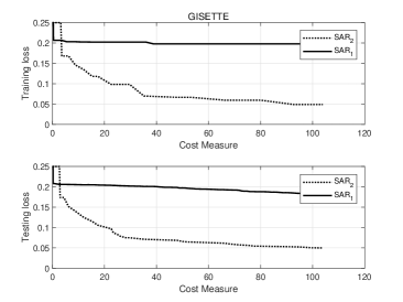
We now solve the binary classification task described at the beginning of Section IV on the MNIST-B and GISETTE datasets, described in Table I. We test the algorithm on both datasets without net, while different ANN structures are considered for the MNIST-B via . A comparison between and is performed on the GISETTE dataset. The accuracy in terms of the binary classification rate on the testing set, for each of the performed methods and ANN structures, is reported in Table II, averaging over 20 runs.
| Dataset | Training | Testing | |
|---|---|---|---|
| GISETTE | |||
| MNIST-B |
| Dataset | ||||
| (no net) | shallow net: | 2-hidden layers | (no net) | |
| net: | ||||
| GISETTE | – | – | ||
| MNIST-B | – |
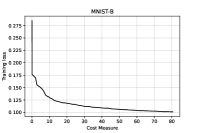
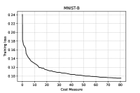
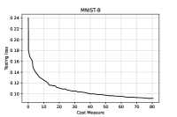
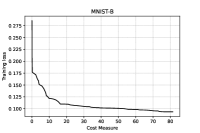
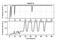
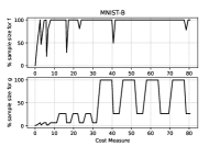
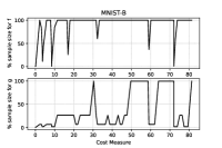
We immediately note that, for the series of tests performed using , adding hidden layers with a small amount of neurons seems to be effective, since the accuracy in the binary classification on the testing set increases. In order to avoid overfitting, no net is considered on the GISETTE dataset, because of the fact that the number of parameters is greater than the number of training samples (see Table I) already in the case of no hidden layers. We further notice that, the second order procedure provides, for the GISETTE dataset, a higher classification accuracy. Therefore, on this test, adding second order information is beneficial. To get more insight, in Figures 1–2 and Figure 5 we plot the training and testing loss against CM, while Figures 3–4 and Figure 6 are reserved to the computed sample sizes, performed by the tested procedures. Concerning the MNIST-B dataset, Figures 1–2 show that the decrease of the training and testing loss against CM performed by goes down to more or less the same values at termination, meaning that the training phase has been particularly effective and thus the method is able of generalising the ability of predicting labels learnt on the training phase when the testing data are considered.


Figures 3–4, reporting the the adaptive sample sizes (in percentage) for computed function and gradient against CM within the algorithm, show that the sample size for estimating the objective function oscillates for a while, flattening on the full sample size eventually. The same is true for the corresponding gradients estimations, even if the growth toward the full sample is slower and the trend often remains below this threshold, especially for the MNIST-B dataset with ANN.
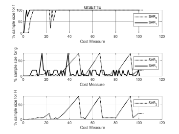
Moving to the GISETTE dataset, Figure 5 makes clear that the use of second order information enables the method to obtain lower values of the training and testing loss, with the same computational effort, and this yields higher classification accuracy. We also note (see Figure 6) that employs only occasionally the of sample to approximate the Hessian matrix and in most of the iterations the Hessian approximation is obtained averaging on less than of samples.
V Conclusions and perspectives
The final expected bounds in (17) are sharp in the order of the tolerances . The effect of inaccurate evaluations is thus limited to scaling the optimal complexity that we would otherwise derive from the deterministic analysis (see, e.g., Theorem 5.5 in [16] and Theorem 4.2 in [5]), by a factor which depends on the probability of the model being accurate. Finally, first promising numerical results within the range of nonconvex finite-sum binary classification for imaging datasets confirm the expected behaviour of the method. From a theoretical perspective, the inclusion of inexact function evaluations subject to random noise is at the moment an open and challenging issue.
Acknowledgment
INdAM-GNCS partially supported the first, second and third author under Progetti di Ricerca 2019 and 2020.
References
- [1] Agarwal, N., Allen-Zhu, Z., Bullins, B., Hazan, E., Ma, T.: Finding approximate local minima faster than gradient descent. In: Proceedings of the 49th Annual ACM SIGACT Symposium on Theory of Computing, pp. 1195–1199 (2017).
- [2] S. Bellavia, T. Bianconcini, N. Krejić, B. Morini, Subsampled first-order optimization methods with applications in imaging. Handbook of Mathematical Models and Algorithms in Computer Vision and Imaging. Springer, to appear.
- [3] Bellavia, S., Gurioli, G., Morini, B., Toint, Ph. L.: High-order Evaluation Complexity of a Stochastic Adaptive Regularization Algorithm for Nonconvex Optimization Using Inexact Function Evaluations and Randomly Perturbed Derivatives. arXiv:2005.04639 (2021).
- [4] Bellavia, S., Gurioli, G.: Complexity Analysis of a Stochastic Cubic Regularisation Method under Inexact Gradient Evaluations and Dynamic Hessian Accuracy. To appear, DOI:10.1080/02331934.2021.1892104 (2021).
- [5] Bellavia, S., Gurioli, G., Morini, B. Adaptive Cubic Regularization Methods with Dynamic Inexact Hessian Information and Applications to Finite-Sum Minimization. IMA Journal of Numerical Analysis 41(1), 764–799 (2021).
- [6] Bellavia, S., Gurioli, G., Morini, M., Toint, Ph. L.: Adaptive Regularization Algorithms with Inexact Evaluations for Nonconvex Optimization. SIAM Journal on Optimization 29(4), 2281–2915 (2019).
- [7] Berahas, A. S., Bollapragada, R., Nocedal, J.: An investigation of Newton-sketch and subsampled Newton methods. Optimization Methods and Software 35(4), 1–20 (2020).
- [8] Berahas, A., Cao, L., Scheinberg, K.: Global convergence rate analysis of a generic line search algorithm with noise. arXiv:1910.04055 (2019).
- [9] C Bertocchi C.,Chouzenoux E. , Corbineau M.C., Pesquet J.C., Prato M.:Deep unfolding of a proximal interior point method for image restoration. Inverse problems, 36, 034005 (2020).
- [10] Bianconcini, T., Liuzzi, G., Morini, B., Sciandrone, M.: On the use of iterative methods in cubic regularization for unconstrained optimization. Computational Optimization and Applications 60(1), 35–57 (2015).
- [11] Birgin, E. G., Gardenghi, J. L., Martínez, J. M., Santos, S. A., Toint, Ph. L.: Worst-case evaluation complexity for unconstrained nonlinear optimization using high-order regularized models. Mathematical Programming Ser. A 163(1–2), 359–368 (2017).
- [12] Blanchet, J., Cartis, C., Menickelly, M., Scheinberg, K.: Convergence rate analysis of a stochastic trust region method via supermartingales. INFORMS Journal on Optimization 1(2), 92–119 (2019).
- [13] Bottou, L. , Curtis, F. E., Nocedal, J.: Optimization Methods for Large-Scale Machine Learning. SIAM Review 60(2), 223–311 (2018).
- [14] Carmon, Y., Duchi, J. C.: Gradient descent efficiently finds the cubic-regularized non-convex Newton step. arXiv preprint arXiv:1612.00547 (2016).
- [15] Carmon, Y., Duchi, J. C., Hinder, O., Sidford, A.: Accelerated methods for nonconvex optimization. SIAM Journal on Optimization 28(2), 1751–1772 (2018).
- [16] Cartis, C., Gould, N. I. M., Toint, Ph. L.: Strong evaluation complexity bounds for arbitrary-order optimization of nonconvex nonsmooth composite functions. arXiv:2001.10802 (2020).
- [17] Cartis, C., Gould, N. I. M., Toint, Ph. L.: Sharp worst-case evaluation complexity bounds for arbitrary-order nonconvex optimization with inexpensive constraints. SIAM Journal on Optimization 30(1), 513–541 (2020).
- [18] Cartis, C., Scheinberg, K.: Global convergence rate analysis of unconstrained optimization methods based on probabilistic models. Mathematical Programming Ser. A 159(2), 337–375 (2018).
- [19] Cartis, C., Gould, N. I. M., Toint, Ph. L.: Complexity bounds for second-order optimality in unconstrained optimization. J. Complex. 28(1), 93–108 (2012).
- [20] Cartis, C., Gould, N. I. M., Toint, Ph. L. : An adaptive cubic regularisation algorithm for nonconvex optimization with convex constraints and its function-evaluation complexity. IMA Journal of Numerical Analysis 32(4), 1662–1695 (2012).
- [21] Cartis, C., Gould, N. I. M., Toint, Ph. L.: Adaptive cubic overestextrmation methods for unconstrained optimization. Part I: motivation, convergence and numerical results. Mathematical Programming Ser. A 127, 245–295 (2011).
- [22] Cartis, C. , Gould, N. I. M., Toint, Ph. L.: Adaptive cubic overestextrmation methods for unconstrained optimization. Part II: worst-case function and derivative-evaluation complexity. Mathematical Programming Ser. A 130(2), 295–319 (2011).
- [23] Chen, X., Jiang, B., Lin, T., Zhang, S.: On Adaptive Cubic Regularized Newton’s Methods for Convex Optimization via Random Sampling. arXiv:1802.05426 (2018).
- [24] Chen, R., Menickelly, M., Scheinberg, K.: Stochastic optimization using a trust-region method and random models. Mathematical Programming Ser. A 169(2), 447–487 (2018).
- [25] , D. di Serafino and V. Ruggiero and G. Toraldo and L. Zanni, On the steplength selection in gradient methods for unconstrained optimization, Applied Mathematics and Computation, vol. 318, pp. 176 - 195, 2018.
- [26] Goodfellow, I., Bengio, Y., Courville, A.: Deep learning, MIT press (2016).
- [27] Kohler, J. M., Lucchi, A..: Sub-sampled cubic regularization for non-convex optimization. Proceedings of the 34th International Conference on Machine Learning 70, 1895–1904 (2017).
- [28] Jin K.H, McCann M.T, Froustey E., Unser M.: Deep convolutional neural network for inverse problems in imaging. IEEE Trans. Image Process. 26 4509–4522 (2017)
- [29] LeCun, Y., Bottou, L., Bengio, Y., Haffner, P.: Gradient-based learning applied to document recognition. Proceedings of the IEEE 86, 2278–2324 (1998).
- [30] M. Lichman. UCI machine learning repository. https://archive.ics.uci.edu/ml/index.php (2013).
- [31] McCann M.T, Jin K.H, Unser M., Convolutional neural networks for inverse problems in imaging: a review. IEEE Signal Process. Mag. 34, 85–95 (2017)
- [32] Paquette, C., Scheinberg, K.: A stochastic line search method with convergence rate analysis. SIAM Journal on Optimization 30(1), 349–376 (2020).
- [33] Pearlmutter, B. A.: Fast exact multiplication by the Hessian. Neural computation 6(1), 147–160 (1994).
- [34] M. Raydan, Journal = SIAM Journal on Optimization, The Barzilai and Borwein gradient method for the large scale unconstrained minimization problem, SIAM Journal on Optimization, vol. 7(1), pp. 26–33, 1997.
- [35] Xu, P., Roosta-Khorasani, F., Mahoney, M. W.: Second-Order Optimization for Non-Convex Machine Learning: An Empirical Study. In: Proceedings of the 2020 SIAM International Conference on Data Mining, pp.199–207 (2020).
- [36] Xu, P., Roosta-Khorasani, F., Mahoney, M. W.: Newton-type methods for non-convex optimization under inexact Hessian information. Mathematical Programming 184, 35–70 (2020).
- [37] Yao, Z., Xu, P., Roosta-Khorasani, F., Mahoney, M. W.: Inexact Non-Convex Newton-type Methods. arXiv:1802.06925 (2018).
- [38] Schraudolph, N. N.: Fast curvature matrix-vector products for second-order gradient descent. Neural computation 14(7), 1723–1738 (2002).
- [39] Shanmugamani, R., Deep Learning for Computer Vision: Expert techniques to train advanced neural networks using TensorFlow and Keras, Packt Publishing (2018).
- [40] Tropp, J.: An Introduction to Matrix Concentration Inequalities. Number 8,1-2 in Foundations and Trends in Machine Learning. Now Publishing, Boston, USA, 2015.
- [41] Zhou, D., Xu, P., Gu, Q. Stochastic Variance-Reduced Cubic Regularization Methods. Journal of Machine Learning Research 20, 1–47 (2019).