Quadratic heptagon cohomology

This paper is the continuation of paper [7] where the first nontrivial heptagon relation was found. We recall here that by heptagon relation, we mean an algebraic imitation of a Pachner move 4–3 in a triangulation of a five-dimensional piecewise linear (PL) manifold, see [10, 9] for Pachner moves and [7, 2, 3, 6, 8] for heptagon and other polygon relations. Discovering heptagon relations may be viewed as a preparational algebraic work for constructing invariants of these manifolds and related topological field theories.

It is known, however, that often more refined invariants can be obtained if we use not only a relation like heptagon but also its cohomology. Enough to mention, as an example, invariants of knots and knotted surfaces coming from just quandles and from quandle cohomology, reviewed in [1].

It can be expected that, for five-dimensional PL manifolds, heptagon 5-cocycles will play the principal role. As explained in [7], we color the 4-faces of a triangulation with elements of a field $F$, and declare some of the colorings for (the faces of) each 5-simplex permitted. Roughly speaking, heptagon itself is expected to give, as a manifold $M$ invariant, the dimension of the vector space of its triangulation’s permitted colorings, corrected by some simple multiplier. Different values $c[M]$ of a heptagon 5-cocycle $c$ on $M$ can add more information to that invariant.

Field $F$ must be big enough to allow for some sets of its elements to be in a ‘general position’, see, for instance, an assumption made below right after formula (3). When speaking of quadratic cohomology, we also assume that its characteristic is not 2. Moreover, for some of our calculations, $F$ must be of characteristic 0, which is explicitly indicated in the relevant places in the text.

The heptagon relation and its cohomology studied here are nonconstant. This means that the specific objects belonging to a simplex (such as e.g. the matrix determining its permitted colorings or the coefficients in the expression for a cocycle) depend on parameters that are different for different simplices. The difference between ‘constant’ and ‘nonconstant’ cohomology theories can be seen on the hexagon example by comparing papers [6] and [8].

The main result of this paper is the existence of a non-trivial 5-cocycle for the heptagon relation introduced in [7], together with explicit algebraic formulas for it. This looks actually quite striking if compared with the apparent non-existence of a similar cocycle for other odd polygon relations of the same kind. Namely, we analyze here also pentagon, enneagon (9-gon) and hendecagon (11-gon).

Recall that the existence of higher (than pentagon and heptagon) odd polygon relations was announced in [7, Subsection 6.3], together with a brief but explicit explanation of the key step for their construction. We still leave their general analysis for future works, but as we want to compare heptagon with pentagon, enneagon and hendecagon, we simply write out necessary formulas for these, and content ourself with the fact that, in these cases, the formulas (including polygon relations as such) can be checked directly using computer algebra.

Anyhow, we could not do without computer algebra altogether, even for the heptagon, both when searching for our 5-cocycle and when checking its validity. This probably means that there are hidden algebraic structures, yet to be discovered.

Aristophanes Dimakis taught me a more elegant, than in [7], way of vertex and simplex numbering in polygon relations, used in [2, 3]. Accordingly, our Pachner move now replaces the cluster of 5-simplices with numbers 1, 3, 5 and 7 with the cluster of 5-simplices 2, 4 and 6. The heptagon looks now as in Figure 1

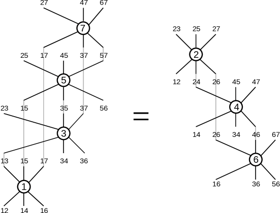
rather than [7, Figure 1], and reads

instead of [7, Eq. (1)]. Note that the subscripts in (1) did not change.

Also, we change the meaning of letter $n$, to bring it in conformity with [3]: our odd polygons are now $(2n+1)$-gons, so $n=2$ for pentagon, $n=3$ for heptagon, and so on.

Below,

• $\bullet$

  in Section 2, we recall our heptagon relation introduced in [7],

• $\bullet$

  in Section 3, we introduce both a general cohomology theory for heptagon and its specific ‘quadratic’ version,

• $\bullet$

  in Section 4, we present a quadratic cocycle in dimension 4, and show its uniqueness,

• $\bullet$

  in Section 5, we present a quadratic cocycle in dimension 5 together with some related reasonings and observations,

• $\bullet$

  in Section 6, we find out that, while analogues of the heptagon 4-cocycle exist for pentagon, enneagon and hendecagon, such analogues of the heptagon 5-cocycle do not exist,

• $\bullet$

  finally, in Section 7, we discuss possible directions of further research.

Recall that (1) and Figure 1 mean the equalness of two products of matrices acting in the direct sum of six copies of field $F$. We represent this direct sum as the 6-row space, so our matrices act on rows from the right. Each matrix $A_{abc}^{(p)}$ acts nontrivially only in the copies (or: on the row elements) number $a$, $b$ and $c$. Circles with numbers in Figure 1 depict the seven 5-simplices taking part in move 4–3, while edges correspond to 4-faces: edge $ij$ depicts the 4-face common for simplices $i$ and $j$, including the case where these belong to the different sides of Figure 1 (recall that the lhs and rhs of a Pachner move have the same boundary). The order of $i$ and $j$ is here, by definition, irrelevant: edge/face $ij$ is the same as $ji$.

It proved also convenient for us to denote the vertices of simplices taking part in the Pachner move by the same letters (or numbers) as 5-simplices, using the following principle: 5-simplex $i$ has all vertices $1,\ldots,7$ except $i$. That is, 5-simplex $1$ can also be denoted as $234567$; accordingly, 4-face $12$ is the same as $34567$.

Note that below, in Subsection 2.3, we speak of edges of these simplices, not to be confused with edges of Figure 1.

Explicitly, entries of matrices $A_{abc}^{(p)}$ are described as follows. First, we introduce a matrix

with entries in $F$, and determinants

made of triples of its columns. We assume that the entries of $\mathcal{M}$ are generic enough in the exact sense that $d_{ijk}$ does not vanish for any pairwise different $i,j,k$.

Each separate matrix $A^{(p)}$ looks as in Figure 2.

By definition, the entry of $A^{(p)}$ corresponding to the input (lower) leg $ip=pi$ and output (upper) leg $lp=pl$ is

where $jp$ and $kp$ are the other input legs of $A^{(p)}$.

It was proved in [7] that matrices (4) satisfy (1).

The main technical tool used in [7] to construct our heptagon relation was edge vectors—permitted colorings of the Pachner move such that nonzero colors are ascribed only to 4-faces containing a given edge $b=ij$. Recall that the explicit expression for the component $e_{b}|_{u}$ of edge vector $e_{b}$ corresponding to 4-face $u$ is

where $l$ and $m$ are the two vertices not belonging to $u$ (while $i$ and $j$, of course, do belong).

Any four vectors $e_{ij},e_{ik},e_{il},e_{im}$ corresponding to edges with a common vertex $i$ are linearly dependent:

where $\lambda_{i,ij}^{(ijklm)}$ are some numbers whose explicit expression is given in [7, Eq. (13)].

In this subsection, we define “nonconstant heptagon cohomology” in a general context.

Our definition will depend on a chosen simplicial complex $K$. In principle, $K$ can be of any dimension, although the main work in this paper will take place in the standard 6-simplex $K=\Delta^{6}$, whose boundary is the union of the lhs and rhs of any five-dimensional Pachner move.

Suppose that every 4-simplex $u\subset K$ is colored by some element $\mathsf{x}_{u}\in X$ of a set $X$ of colors (for instance, our field $X=F$), and that a subset $R_{v}$ of permitted colorings is defined in the set of all colorings of every 5-simplex $v$ (for instance, by declaring that the “output” colors must be determined by the “input” ones, using matrix (4)).

We also define the set of permitted colorings for any simplex of $K$ of dimension $>5$: the coloring is permitted provided its restrictions on all 5-faces of that simplex are permitted. As for an individual 4-simplex, all its colorings $\mathsf{x}\in X$ are permitted by definition.

The set of all permitted colorings of an $m$-simplex $i_{0}\dots i_{m}$ will be denoted $\mathfrak{C}_{i_{0}\dots i_{m}}$. We assume here that the vertices of any simplex are ordered: $i_{0}<\ldots<i_{m}$.

Let an abelian group $G$ be given. By definition, an $m$-cochain $\mathfrak{c}$ taking values in $G$, for $m\geq 3$, consists of arbitrary mappings

for all $m$-simplices $\Delta^{m}=i_{0}\dots i_{m}\subset K$.

The coboundary $\delta\mathfrak{c}$ of $\mathfrak{c}$ consists then of mappings $(\delta\mathfrak{c})_{i_{0}\dots i_{m+1}}$ acting on a permitted coloring $r\in\mathfrak{C}_{i_{0}\dots i_{m+1}}$ of $(m+1)$-simplex $i_{0}\dots i_{m+1}$ according to the following formula:

where each $r|_{i_{0}\dots\widehat{i_{k}}\dots i_{m+1}}$—the restriction of $r$ onto the $m$-simplex $i_{0}\dots\widehat{i_{k}}\dots i_{m+1}$—is of course a permitted coloring of this latter simplex.

Our ‘nonconstant heptagon cohomology’ is the cohomology of the following heptagon cochain complex:

where $C^{m}$ means the group of all $m$-cochains.

It turns out that there are some interesting variations of the cochain definition (7). For instance, preprint [6] (although devoted to constant hexagon cohomology) suggests that homogeneous polynomials of a given degree may be used instead of general functions (7)—of course, in a situation where the notion of polynomial in the variables determining a permitted coloring makes sense.

Of special interest for us in this paper will be quadratic cochains. That is, let $G=F$ be the same field $F$ that we are using for the set of colors, and mappings $\mathfrak{c}_{i_{0}\dots i_{m}}$ in (7) be quadratic forms on the linear spaces of permitted colorings of corresponding $m$-simplices $i_{0}\ldots i_{m}$.

Remember (Subsection 1.1) that our field $F$ is of characteristic $\neq 2$. Hence, there is a polarization for any quadratic cochain. By definition, this is the symmetric bilinear cochain depending on two (independent from each other) permitted colorings:

where each $\mathfrak{c}_{i_{0}\dots i_{m}}^{\mathrm{pol}}$ is the polarization of the corresponding $\mathfrak{c}_{i_{0}\dots i_{m}}$ in (7).

Mapping (10) can be treated as a scalar product of two permitted colorings of simplex $i_{0}\dots i_{m}$. So, to define a quadratic cochain is essentially the same as to define a scalar product for all corresponding simplices. In what follows, we will make extensive use of this fact.

We first calculate the numbers of linearly independent quadratic 4-, 5- and 6-cochains in our simplicial complex $K=\Delta^{6}=1234567$.

We define now one more scalar product, this time between two permitted colorings of a 5-simplex $p$. For the case where these colorings are the restrictions of edge vectors $e_{ij}$ and $e_{kl}$, respectively, on $p$, we set

where

and $i,\ldots,n$ are the numbers from 1 through 7 except $p$, going in the increasing order.

As edge vectors make not a basis but an overfull system of vectors in the linear space of all permitted colorings, the following proposition is necessary to justify this definition.

Matrix $\mathcal{M}$ (2) can be reduced, by a linear transformation of its rows, to the form where its three first columns form an identity matrix. Suppose this has been already done, that is,

and consider the determinant of matrix $\eta_{7}$ (16) for such $\mathcal{M}$. A calculation shows that

where function ‘$\operatorname{dh}$’ on $3\times 3$ matrices was introduced in [5, Eq. (7)] in connection with what seemed a completely different problem—evolution of a discrete-time dynamical system, where one step of evolution consisted in taking, first, the usual inverse of a matrix, and second—the “Hadamard inverse”, that is, inverting each matrix entry separately.

It was announced in [7, Subsection 6.3] that our heptagon relation can be generalized to any $(2n+1)$-gon, $n=2,3,\ldots$. The form of such relations has been explained in detail in [3, Section II.B] (while different $(2n+1)$-gon relations of the same form were presented in [3, Section III]).

Here we want only to comment on the results of computer calculations for pentagon, enneagon (9-gon) and hendecagon (11-gon). This allows us just to say that all mentioned polygon relations do hold, and this can be checked directly using computer algebra, if we set the entries of the corresponding matrices $A^{(p)}$ to have the following entries:

In greater detail: the product in (25) runs over all $j$ such that the lower (input) legs of $A^{(p)}$ are marked $jp$, except $j=i$, see again Figure 2 for the heptagon example. The determinants $d_{ijk}$ are the same as in (3), except that matrix $\mathcal{M}$ (2) must have $2n+1$ columns (but still three rows).

Our definition (25) generalizes (4), of course. It works actually for all $(2n+1)$-gons, but the proof of this general fact (not relying on computer algebra) will appear elsewhere.

Nontrivial $(2n-2)$-cocycles are given, for a general $n$, by the very same formulas (11) and (12). The conceptual and general proof of this statement—a generalization of our Proposition 1—requires, however, some preparatory work, and we leave it for a future paper specifically addressing these issues. As far as only pentagon, enneagon and hendecagon relations are concerned, it can be checked quite easily using computer algebra.

Their uniqueness—the generalization of Proposition 2—also holds, and this time not much work is required. For clarity, we show how to do it on the example of enneagon. According to [7, Subsection 6.3], edge vectors are replaced, for enneagon, with triangle vectors. Consider 7-simplex 12345678—also denoted simply ‘9’—and triangle vectors for 123 and 456. The mentioned 7-simplex contains only two 6-faces, namely $1234567$ and $1234568$, also called $89$ and $79$, containing both these triangles. Scalar product $\langle e_{123},e_{456}\rangle_{6}^{(9)}$—the analogue of $\langle e_{12},e_{34}\rangle_{4}^{(7)}$ from the proof of Proposition 2—must vanish, and this determines $c_{79}/c_{89}$ uniquely. Similarly, all ratios between coefficients $c_{ip}$ are also determined uniquely.

We now write out the analogues of sequence (14) for pentagon, enneagon and hendecagon, assuming again the zero characteristic for field $F$.

References

- [1] Scott Carter, Seiichi Kamada, Masahico Saito, Surfaces in 4-space, Encyclopaedia of Mathematical Sciences, Volume 142, Springer 2004.
- [2] Aristophanes Dimakis and Folkert Müller-Hoissen, Simplex and polygon equations, SIGMA 11 (2015), paper 042, 49 pages.
- [3] Aristophanes Dimakis and Igor G. Korepanov, Grassmannian-parameterized solutions to direct-sum polygon and simplex equations, J. Math. Phys. 62 (2021), 051701.
- [4] Allen Hatcher, Algebraic topology, Cambridge University Press, 2002.
- [5] I.G. Korepanov, Exact solutions and mixing in an algebraic dynamical system, Theoretical and Mathematical Physics, 143:1 (2005), 599–614.
- [6] I.G. Korepanov, N.M. Sadykov, Hexagon cohomologies and polynomial TQFT actions, arXiv:1707.02847.
- [7] I.G. Korepanov, Heptagon relation in a direct sum, Algebra i Analiz, 33:4 (2021), 125–140 (Russian). English translation: arXiv:2003.10335.
- [8] Igor G. Korepanov, Nonconstant hexagon relations and their cohomology, Lett. Math. Phys. 111, paper 1 (2021), arXiv:1812.10072.
- [9] W.B.R. Lickorish, Simplicial moves on complexes and manifolds, Geom. Topol. Monogr. 2 (1999), 299–320. arXiv:math/9911256.
- [10] U. Pachner, PL homeomorphic manifolds are equivalent by elementary shellings, Europ. J. Combinatorics 12 (1991), 129–145.