Quantification of Risk in Classical Models of Finance

Alois Pichler Funded by Deutsche Forschungsgemeinschaft (DFG, German Research Foundation) – Project-ID 416228727 – SFB 1410 Ruben Schlotter Both authors: Technische Universität Chemnitz, 09126 Chemnitz, Germany. Contact: ruben.schlotter@math.tu-chemnitz.de

Abstract

This paper enhances the pricing of derivatives as well as optimal control problems to a level comprising risk. We employ nested risk measures to quantify risk, investigate the limiting behavior of nested risk measures within the classical models in finance and characterize existence of the risk-averse limit. As a result we demonstrate that the nested limit is unique, irrespective of the initially chosen risk measure. Within the classical models risk aversion gives rise to a stream of risk premiums, comparable to dividend payments. In this context we connect coherent risk measures with the Sharpe ratio from modern portfolio theory and extract the Z-spread—a widely accepted quantity in economics to hedge risk.

The results for European option pricing are then extended to risk-averse American options, where we study the impact of risk on the price as well as the optimal time to exercise the option.

We also extend Merton’s optimal consumption problem to the risk-averse setting.

Keywords: Risk measures, Optimal control, Black–Scholes

Classification: 90C15, 60B05, 62P05

1 Introduction

This paper studies discrete classical models in finance under risk aversion and their behavior in a high-frequency setting. Using nested risk measures we first study risk aversion in the multiperiod model.

We develop risk aversion in a discrete time and discrete space setting and find an important consistency property of nested risk measures. This consistency property, termed divisibility, is crucial in high-frequency trading environments. For this, our study of risk-averse models extends to continuous time processes as well. This very property allows consistent decision making, i.e., decisions, which are independent of individually chosen discretizations or trading frequencies. Our results also give rise to a generalized Black–Scholes framework, which incorporates risk aversion in addition.

Riedel (2004) has introduced risk measures in a dynamic setting. Later, Cheridito et al. (2004) study risk measures for bounded càdlàg processes and Cheridito et al. (2006) also discuss risk measures in a discrete time setting. Ruszczyński and Shapiro (2006) introduce nested risk measures, for which Philpott et al. (2013) provide an economic interpretation as an insurance premium on a rolling horizon basis. For a recent discussion on risk measures and dynamic optimization we refer to De Lara and Leclère (2016). Applications can be found in Philpott and de Matos (2012) or Maggioni et al. (2012), e.g., where stochastic dual dynamic programming methods are addressed, see also Guigues and Römisch (2012).

Divisibility is an indispensable prerequisite in defining an infinitesimal generator based on discretizations. This generator, called risk generator, constitutes the risk-averse assessment of the dynamics of the underlying stochastic process. Using the risk generator we characterize the existence of the risk-averse limit of discrete pricing models. For coherent risk measures and Itô diffusion processes the risk generator constitutes a nonlinear operator, comparable to the classical infinitesimal generator but with an additional term, accounting for risk, which takes the form

s_{\rho}\,\left|\sigma\,\partial_{x}\,(\cdot)\right|.

Here, $s_{\rho}$ is a scalar expressing the degree of risk aversion and $\sigma$ is the volatility of the diffusion process describing the asset price. It turns out that the risk generator only depends on the risk measure through the coefficient of risk aversion $s_{\rho}$ . This surprising feature has important conceptual implications, as evaluating a risk measure is often an optimization problem itself. As well we derive that the scaling quantity $s_{\rho}$ allows the economic interpretation of a Sharpe ratio and $s_{\rho}\cdot\sigma$ is the Z-spread.

Using the risk generator we derive a nonlinear Black–Scholes equation, which we relate to the Black–Scholes formula for dividend paying stocks proposed by Merton (1973). Moreover we relate risk-averse pricing models to foreign exchange options models as in Garman and Kohlhagen (1983). Nonlinear Black–Scholes equations have been discussed previously in Barles and Soner (1998) and Ševčovič and Žitňanská (2016) in the context of modeling transaction costs. There, the nonlinearity is in the second derivative. In contrast, risk aversion leads to drift uncertainty and causes nonlinearity in the first derivative.

Very different to our approach, Stadje (2010) studies the convergence properties of discretizations of dynamic risk measures based on backwards stochastic differential equations introduced in Pardoux and Peng (1990) (see also Delong (2013) for an overview). Ruszczyński and Yao (2015) then derive risk-averse Hamilton–Jacobi–Bellmann equations based on these backwards stochastic differential equations.

For coherent risk measures we derive an explicit solution for the European option pricing problem. We show that risk aversion expressed via coherent risk measures can be interpreted either as an extra dividend payment or capital injection. Furthermore we relate risk-aversion to a change of currency as in the foreign exchange option model. The amount of the dividend payment or, equivalently, the interest rate in the risk-averse currency, is given by a multiple of the Sharpe ratio and the volatility of the underlying stock. This ratio, which expresses risk aversion, arises for any coherent risk measure and does not depend on a specific market model such as the Black–Scholes model. However, as our focus is on classical models, we restrict ourselves to Itô diffusion processes.

Using a free boundary formulation we extend the analysis from European to American option pricing. For the Black–Scholes option pricing of European and American options, risk-aversion naturally leads to a bid-ask spread, which we quantify explicitly.

Similarly we extend the Merton optimal consumption problem to a risk-averse setting. We elaborate on the optimal controls and show that risk-aversion reduces the investment in risky assets and increases consumption. We observe the same pattern as for European and American options, that is, risk-aversion corrects the drift of the underlying market model. For all classical models discussed here, the risk-averse assessment still allows explicit pricing and control formulae.

2 Preliminaries on risk measures

Recall the definition of law invariant, coherent risk measures $\rho\colon L\to\mathbb{R}$ defined on some vector space $L$ of $\mathbb{R}$ -valued random variables first. They satisfy the following axioms introduced by Artzner et al. (1999).

A1.

Monotonicity: $\rho(Y)\leq\rho(Y^{\prime})$ , provided that $Y\leq Y^{\prime}$ almost surely;
A2.

Translation equivariance: $\rho(Y+c)=\rho(Y)+c$ for $c\in\mathbb{R}$ ;
A3.

Subadditivity: $\rho\big{(}Y+Y^{\prime}\big{)}\leq\rho(Y)+\rho(Y^{\prime})$ ;
A4.

Positive homogeneity: $\rho(\lambda\,Y)=\lambda\,\rho(Y)$ for $\lambda\geq 0$ ;

A5.

Law invariance: $\rho(Y)=\rho(Y^{\prime})$ , whenever $Y$ and $Y^{\prime}$ have the same law, i.e., $P(Y\leq y)=P(Y^{\prime}\leq y)$ for all $y\in\mathbb{R}$ .

The expectation ( $\rho(Y)=\operatorname{{\mathds{E}}}Y$ ) is also a law invariant coherent risk measure, expressing risk-neutral behavior. In contrast to the risk-neutral setting, the risk-averse setting distinguishes between $\rho(Y)$ and $-\rho(-Y)$ . As a result of¹¹1The inequality $0=\rho(Y-Y)\leq\rho(Y)+\rho(-Y)$ implies that $-\rho(-Y)\leq\rho(Y)$ .

-\rho(-Y)\leq\rho(Y)

we will later identify $\rho(Y)$ with the seller’s ask price and $-\rho(-Y)$ with the buyer’s bid price in the option pricing problems discussed below.

2.1 Nested risk measures

We consider a filtered probability space $\left(\Omega,\mathcal{F},(\mathcal{F}_{t})_{t\in\mathcal{T}},P\right)$ and associate $t\in\mathcal{T}$ with stage or time. For the discussion of risk in a dynamic setting we introduce nested risk measures corresponding to the evolution of risk over time. Nested risk measures are compositions of conditional risk measures (cf. Pflug and Römisch (2007)).

Recall that a coherent risk measures $\rho\colon L\to\mathbb{R}$ can be represented by

\rho(Y)=\sup_{Q\in\mathcal{Q}}\,\operatorname{{\mathds{E}}}_{Q}Y,

(1)

where $\mathcal{Q}$ is a convex set of probability measures absolutely continuous with respect to $P$ (cf. also Delbaen (2002)). We assume throughout that $\rho\colon L^{p}\to\mathbb{R}$ for some fixed $p\geq 1$ . Following Ruszczyński and Shapiro (2006), we then introduce conditional versions $\rho^{t}\colon L^{p}\to L^{p}(\Omega,\mathcal{F}_{t},P)$ of the risk measure $\rho$ conditioned on the sigma algebra $\mathcal{F}_{t}$ . Note that the conditional risk measures $\rho^{t}$ satisfy conditional versions of the Axioms A1–A5 above. For the construction of $\rho^{t}$ and further details we refer the interested reader also to Shapiro et al. (2014, Section 6.8.2).

We now introduce nested risk measures in discrete time.

Definition 1 (Nested risk measures).

The nested risk measure for the partition $\mathcal{P}=\left(t_{0},t_{1},\dots,t_{n}\right)$ at times $t_{0}<\ldots<t_{n}$ is

\rho^{\mathcal{P}}(Y)\coloneqq\rho^{t_{0}}\left(\rho^{t_{1}}\left(\ldots\rho^{t_{n}}(Y)\ldots\right)\right),

(2)

where $(\rho^{t_{i}})_{i=0}^{n}$ is a family of conditional risk measures.

Similar as above, we distinguish the buyer’s and seller’s perspective and consider the bid price

-\rho^{\mathcal{P}}(-Y)=-\rho^{t_{0}}\left(\rho^{t_{1}}\left(\ldots\rho^{t_{n}}(-Y)\ldots\right)\right),

as well as the ask price in (2).

2.2 Nested risk measures for discrete processes

To elaborate key properties of nested risk measures as defined in (2) we discuss the binomial model, well-known from finance, by employing the mean semi-deviation, a coherent risk measure satisfying all Axioms A1–A5 above. Particularly, we expose that only specific choices of parameters can lead to consistent models.

Definition 2 (Semi-deviation).

The mean semi-deviation risk measure of order $p\geq 1$ and $Y\in L^{p}$ at level $\beta\in[0,1]$ is

\operatorname{\mathsf{SD}}_{p,\beta}(Y):=\operatorname{{\mathds{E}}}Y+\beta\left\|\left(Y-\operatorname{{\mathds{E}}}Y\right)_{+}\right\|_{p}.

The binomial model.

Consider the stochastic process $S=(S_{0},\dots,S_{T})$ with initial state $S_{0}$ and Markovian transitions with

P\left(S_{t+\Delta t}=S_{t}\cdot e^{\pm\sigma\sqrt{\Delta t}}\right)=p_{\pm},

(3)

where

p_{+}:=p:=\frac{e^{r\Delta t}-e^{-\sigma\sqrt{\Delta t}}}{e^{\sigma\sqrt{\Delta t}}-e^{-\sigma\sqrt{\Delta t}}}\text{ and }p_{-}:=1-p_{+}.

It holds that $\operatorname{{\mathds{E}}}S_{t+\Delta t}=pS_{t}e^{\sigma\sqrt{\Delta t}}+(1-p)S_{t}e^{-\sigma\sqrt{\Delta t}}=S_{t}e^{r\Delta t}$ . In stochastic finance, the process $S$ models the evolution of a stock over time with respect to the risk-neutral risk measure, where $r$ is the risk free interest rate.

(a) single stage

(b) multistage

Figure 1: Binomial option pricing model

We can evaluate various classical coherent risk measures for this binomial model explicitly. The following remark addresses the mean semi-deviation for the one-period binomial model (cf. Figure 1a) as well as the nested mean semi-deviation for the $n$ -period model in (Figure 1b).

Remark 3 (The mean semi-deviation for the binomial model).

Consider the single stage setting in Figure 1a first. The risk-averse bid price for the stock $S_{\Delta t}$ employing the mean semi-deviation $\operatorname{\mathsf{SD}}_{1,\beta}$ of order $1$ with risk level $\beta$ in the binomial model is

	$\displaystyle-\operatorname{\mathsf{SD}}_{1,\beta}(-S_{\Delta t})$	$\displaystyle=\operatorname{{\mathds{E}}}S_{\Delta t}-\beta\operatorname{{\mathds{E}}}\left(-S_{\Delta t}+\operatorname{{\mathds{E}}}S_{\Delta t}\right)_{+}$
		$\displaystyle=pS_{0}e^{\sigma\sqrt{\Delta t}}+(1-p)S_{0}e^{-\sigma\sqrt{\Delta t}}-\beta\,p(1-p)\left(S_{0}e^{\sigma\sqrt{\Delta t}}-S_{0}e^{-\sigma\sqrt{\Delta t}}\right).$

Involving the new probability weights

\displaystyle\widetilde{p}

\displaystyle:=p\big{(}1-\beta(1-p)\big{)}

(4)

we find

-\operatorname{\mathsf{SD}}_{1,\beta}(-S_{\Delta t})=\widetilde{\operatorname{{\mathds{E}}}}S_{\Delta t}.

We now repeat this observation in $n$ stages and consider an $n$ -period binomial model with step size $\Delta t\coloneqq\frac{T}{n}$ , i.e., $\mathcal{P}=\left(0,\Delta t,2\Delta t,\dots,T\right)$ , cf. Figure 1b. The nested mean semi-deviation for the vector of constant risk levels $\beta=(\widetilde{\beta},\dots,\widetilde{\beta})>0$ satisfies

-\operatorname{\mathsf{SD}}_{1,\beta}^{\mathcal{P}}(-S_{T})=-\operatorname{\mathsf{SD}}_{1,\widetilde{\beta}}\left(\dots\operatorname{\mathsf{SD}}_{1,\widetilde{\beta}}\left(-S_{T}\right)\dots\right)=\widetilde{\operatorname{{\mathds{E}}}}S_{T},

where the last expectation is with respect to the probability measure

\widetilde{P}\left(S_{T}=S_{0}e^{\sigma\left(2k\sqrt{\Delta t}-n\sqrt{\Delta t}\right)}\right)=\binom{n}{k}\widetilde{p}^{k}(1-\widetilde{p})^{n-k},\qquad k=0,\dots,n.

The limit

\frac{1}{\sqrt{n\,\widetilde{p}(1-\widetilde{p})}}\left(\frac{\frac{1}{\sigma}\log\frac{S_{T}}{S_{0}}+n\sqrt{\Delta t}}{2\sqrt{\Delta t}}-n\,\widetilde{p}\right)

(5)

is non-degenerate for $n\to\infty$ , provided that $\widetilde{p}\to\frac{1}{2}$ . Based on the central limit theorem, the limit (5) then follows a standard normal distribution.

Hence, specific choices of the parameter $\beta$ in (4) depending on the discretization have to be considered. To this end we introduce the notion of divisible families of risk measures below and return to this example in Section 4.3.

3 The risk-averse limit of discrete option pricing models

Most well-known coherent risk measures in the literature as the Average Value-at-Risk, the Entropic Value-at-Risk as well as the mean semi-deviation involve a parameter which accounts for the degree of risk aversion. As Remark 3 elaborates, the nested risk-averse binomial model does not necessarily lead to a well-defined limit. It is essential to relate the coefficient of risk aversion of the conditional risk measures to its time period. We therefore introduce the notion of divisible coherent risk measures. The divisibility property is central in discussing the limiting behavior of risk-averse economic models.

Definition 4 (Divisible families of risk measures).

Let $p\geq 1$ be fixed. A family $\rho=\left\{\left.\rho_{\Delta t}\colon L^{p}\to\mathbb{R}\right|\Delta t>0\right\}$ of coherent measures of risk is called divisible, if the following two conditions are satisfied:

1.

For $W\sim\mathcal{N}(0,1)$ normally distributed,

$\lim_{\Delta t\downarrow 0}\,\frac{\rho_{\Delta t}(\sqrt{\Delta t}\cdot W)}{\Delta t}=s_{\rho}$ (6)

for some $s_{\rho}\geq 0$ .
2.

Moreover there is a constant $C>0$ (independent of $Y$ and $\Delta t$ ) such that

$\rho_{\Delta t}(Y)\leq C\sqrt{\Delta t}\left\|Y\right\|_{p}$

for all $Y\in L^{p}$ with $\operatorname{{\mathds{E}}}Y=0$ .

We call a nested risk measure $\rho^{\mathcal{P}}$ divisible if every conditional risk measure is divisible, i.e., the limit in (6) holds for random variables which are conditionally normally distributed and

\rho_{\Delta t}^{t}(Y)\leq C\sqrt{\Delta t}\operatorname{{\mathds{E}}}\big{(}\left|Y\right|^{p}\mid\mathcal{F}_{t}\big{)}^{\frac{1}{p}}

for some constant $C>0$ .

Remark 5.

The (conditional) expectation is divisible with $s_{\mathbb{E}}=0$ . For many other risk measures, the parameters can be adjusted. Candidates for risk measures satisfying this condition are spectral risk measures for which the spectral density is bounded in the $L^{q}$ norm for $q=\frac{p}{p-1}$ . The mean semi-deviation risk measure satisfies the divisibility property as well.

Lemma 6.

For $p\geq 1$ and $\beta\geq 0$ , the family

\left\{\operatorname{\mathsf{SD}}_{p,\beta;\Delta t}:=\operatorname{\mathsf{SD}}_{p,\beta\cdot\sqrt{\Delta t}}\right\},\quad\Delta t>0,

of mean semi-deviations is divisible with limit

s_{\operatorname{\mathsf{SD}}_{p,\beta}}=\beta\left(2\pi\right)^{-\frac{1}{2p}}2^{\frac{1}{2}-\frac{1}{2p}}\cdot\Gamma\left(\frac{p+1}{2}\right)^{\frac{1}{p}}.

Proof.

The second part of Definition 4 is satisfied as for $Y\in L^{p}$ such that $\operatorname{{\mathds{E}}}Y=0$ we have

\operatorname{\mathsf{SD}}_{\beta\sqrt{\Delta t},p}(Y)=\beta\sqrt{\Delta t}\left\|Y_{+}\right\|_{p}\leq\beta\sqrt{\Delta t}\left\|Y\right\|_{p}.

Let $W\sim\mathcal{N}(0,1)$ , then

\displaystyle\operatorname{{\mathds{E}}}\left(\sqrt{\Delta t}W_{+}\right)^{p}

\displaystyle=\int_{\mathbb{R}}\max(w,0)^{p}\cdot\frac{1}{\sqrt{2\pi\Delta t}}e^{-\frac{w^{2}}{2\Delta t}}\,\mathrm{d}w=\frac{1}{\sqrt{2\pi\Delta t}}\int_{0}^{\infty}w^{p}\cdot e^{-\frac{w^{2}}{2\Delta t}}\,\mathrm{d}w.

Employing the Gamma function, the latter integral is

\displaystyle\frac{1}{\sqrt{2\pi\Delta t}}\int_{0}^{\infty}w^{p}\cdot e^{-\frac{w^{2}}{2\Delta t}}\,\mathrm{d}w

\displaystyle=\frac{1}{\sqrt{2\pi}}2^{\frac{p-1}{2}}\Gamma\left(\frac{p+1}{2}\right)\Delta t^{\frac{p}{2}}.

Taking the $p$ -th root and multiplying by $\beta\sqrt{\Delta t}$ we obtain

\frac{\operatorname{\mathsf{SD}}_{p,\beta\sqrt{\Delta t}}(\sqrt{\Delta t}W)}{\Delta t}=\beta\left(2\pi\right)^{-\frac{1}{2p}}2^{\frac{1}{2}-\frac{1}{2p}}\cdot\Gamma\left(\frac{p+1}{2}\right)^{\frac{1}{p}},

the assertion. ∎

We now extend nested risk measures to continuous time and demonstrate that the extension is well-defined for divisible families of risk measures. As a result, we show that the risk-averse binomial option pricing model converges exactly for divisible families of risk measures.

Definition 7 (Nested risk measures).

Let $T>0$ , $t\in[0,T)$ and let $\rho^{\mathcal{P}}$ be divisible for every partition $\mathcal{P}\subset[t,T]$ , cf. Definition 1. The nested risk measure $\rho^{t:T}$ in continuous time for a random variable $Y$ is

\rho^{t:T}\left(Y\left|\,\mathcal{F}_{t}\right.\right):=\lim_{\mathcal{P}\subset[t,T]}\,\rho^{\mathcal{P}}\left(Y\left|\,\mathcal{F}_{t}\right.\right)\qquad\text{almost surely},

(7)

where the almost sure limit is among all partitions $\mathcal{P}\subset[t,T]$ with mesh size $\left\|\mathcal{P}\right\|\coloneqq\max_{i=1,\dots,n}t_{i}-t_{i-1}$ tending to zero for those random variables $Y$ , for which the limit exists.

The following proposition evaluates the nested mean-semideviation for the Wiener process, the basic building block of diffusion processes and thus illustrates the main purpose of the divisibility condition.

Proposition 8 (Nested mean semi-deviation for the Wiener process).

Let $W=(W_{t})_{t\in\mathcal{P}}$ be a Wiener process and $\mathcal{P}=\left(t_{0},t_{1},\dots,t_{n}\right)$ a partition of $[0,T]$ with $\Delta t_{i}:=t_{i+1}-t_{i}$ . For the family of conditional risk measures $\left(\operatorname{\mathsf{SD}}_{p,\beta_{t_{i}}\cdot\sqrt{\Delta t_{i}}}(\cdot\mid\mathcal{F}_{t_{i}})\right)_{t_{i}\in\mathcal{P}}$ , the nested mean semi-deviation is

\operatorname{\mathsf{SD}}_{p,\beta}^{\mathcal{P}}(W_{T})=\sum_{i=0}^{n-1}\beta_{t_{i}}\Delta t_{i}\cdot\left(2\pi\right)^{-\frac{1}{2p}}2^{-\frac{1}{2}}\Gamma\left(\frac{p+1}{2}\right)^{\frac{1}{p}},

(8)

where $\beta=(\beta_{t_{0}},\dots,\beta_{t_{n}})$ is a vector of risk levels.

Proof.

Note that $W_{t_{i+1}}-W_{t_{i}}\sim\mathcal{N}(0,t_{i+1}-t_{i})$ and the conditional mean semi-deviation is (using conditional translation equivariance A2)

\displaystyle\operatorname{\mathsf{SD}}_{p,\beta_{t_{i}}\cdot\sqrt{\Delta t_{i}}}\left(W_{t_{i+1}}\left|\,W_{t_{i}}\right.\right)

\displaystyle=W_{t_{i}}+\operatorname{\mathsf{SD}}_{p,\beta_{t_{i}};\sqrt{\Delta t_{i}}}\left(W_{t_{i+1}}-W_{t_{i}}\left|\,W_{t_{i}}\right.\right).

As Brownian motion has independent and stationary increments with mean zero the calculation in the proof of Lemma 6 shows that

\displaystyle\operatorname{\mathsf{SD}}_{p,\beta_{t_{i}}\cdot\sqrt{\Delta t_{i}}}\left(W_{t_{i+1}}\left|\,W_{t_{i}}\right.\right)

\displaystyle=W_{t_{i}}+\beta_{t_{i}}\Delta t_{i}\cdot\left(2\pi\right)^{-\frac{1}{2p}}2^{-\frac{1}{2}}\Gamma\left(\frac{p+1}{2}\right)^{\frac{1}{p}}.

Iterating as in Definition 1 shows

\displaystyle\operatorname{\mathsf{SD}}_{p,\beta}^{\mathcal{P}}(W_{T})

\displaystyle=\sum_{i=0}^{n-1}\beta_{t_{i}}\Delta t_{i}\cdot\left(2\pi\right)^{-\frac{1}{2p}}2^{-\frac{1}{2}}\Gamma\left(\frac{p+1}{2}\right)^{\frac{1}{p}},

the assertion. ∎

Remark 9.

For constant risk levels $\beta_{t_{i}}=\widetilde{\beta}$ we obtain

\operatorname{\mathsf{SD}}_{p,\beta}^{\mathcal{P}}(W_{T})=\sum_{i=0}^{n-1}\Delta t_{i}\cdot\widetilde{\beta}\cdot\left(2\pi\right)^{-\frac{1}{2p}}2^{-\frac{1}{2}}\Gamma\left(\frac{p+1}{2}\right)^{\frac{1}{p}}=T\cdot s_{\operatorname{\mathsf{SD}}_{p,\widetilde{\beta}}},

the accumulated risk grows linearly in time.

3.1 The risk generator

This section addresses nested risk measures for Itô processes. Furthermore, we characterize convergence under risk using a natural condition involving normal random variables and introduce a nonlinear operator, the risk generator, which also allows discussing risk-averse optimal control problems.

It is well-known that the binomial model in Figure 1b converges to the geometric Brownian motion. We therefore discuss Itô processes $(X_{s})_{s\in\mathcal{T}}$ solving the stochastic differential equation

	$\displaystyle\mathrm{d}X_{s}$	$\displaystyle=b(s,X_{s})\,\mathrm{d}s+\sigma(s,X_{s})\,\mathrm{d}W_{s},\quad s\in\mathcal{T},$		(9)
	$\displaystyle X_{t}$	$\displaystyle=x$

for $\mathcal{T}=[t,\,T]$ . We assume that $X$ following (9) is well-defined and satisfy the so-called usual conditions of Øksendal (2003, Theorem 5.2.1).

We introduce the risk generator for divisible families of coherent risk measures. The risk generator describes the momentary evolution of the risk of the stochastic process.

Definition 10 (Risk generator).

Let $X=(X_{t})_{t}$ be a continuous time process and $(\rho_{\Delta t})_{\Delta t}$ be a family of divisible risk measures. The risk generator based on $(\rho_{\Delta t})_{\Delta t}$ is

\mathcal{R}_{\rho}\Phi(t,x):=\lim_{\Delta t\downarrow 0}\frac{1}{\Delta t}\Bigl{(}\rho_{\Delta t}\bigl{(}\Phi(t+\Delta t,X_{t+\Delta t})\left|\,X_{t}=x\right.\bigr{)}-\Phi(t,x)\Bigr{)}

(10)

for those functions $\Phi\colon\mathcal{T}\times\mathbb{R}\to\mathbb{R}$ , for which the limit exists.

Using the ideas from Proposition 8 we obtain explicit expressions for the risk generator for Itô diffusion processes.

Proposition 11 (Risk generator).

Let the family $(\rho_{\Delta t})_{\Delta t}$ be divisible for some $p\geq 1$ fixed. Let $X$ be the solution of (9) and $\Phi\in C^{2}(\mathcal{T}\times\mathbb{R})$ such that $\sigma\,\Phi_{x}$ is Hölder continuous for $\alpha>0$ in $p$ -th mean, i.e., there exists $C>0$ such that $\operatorname{{\mathds{E}}}C^{p}<\infty$ and

\left|\left(\sigma\,\Phi_{x}\right)(t,X_{t})-\left(\sigma\,\Phi_{x}\right)(s,X_{s})\right|\leq C\cdot\left|t-s\right|^{\alpha},\qquad s,t\in\mathcal{T}.

(11)

Then the risk generator based on $(\rho_{\Delta t})_{\Delta t}$ is given by the nonlinear differential operator

\displaystyle\mathcal{R}_{\rho}\Phi(t,x)

\displaystyle=\left(\Phi_{t}+b\,\Phi_{x}+\frac{\sigma^{2}}{2}\Phi_{xx}+s_{\rho}\cdot\left|\sigma\,\Phi_{x}\right|\right)(t,x).

(12)

Remark 12.

In the appendix we provide a sufficient condition for the Assumption (11).

Proof.

By assumption, $\Phi\in C^{2}(\mathcal{T}\times\mathbb{R})$ and hence we may apply Itô’s formula. For convenience and ease of notation we set $f_{1}(t,x):=\left(\Phi_{t}+b\,\Phi_{x}+\frac{\sigma^{2}}{2}\Phi_{xx}\right)(t,x)$ and $f_{2}(t,x):=\left(\sigma\,\Phi_{x}\right)(t,x)$ . In this setting, Eq. (10) rewrites as

\displaystyle\mathcal{R}_{\rho}\Phi(t,x)

\displaystyle=\lim_{\Delta t\downarrow 0}\,\frac{1}{\Delta t}\rho_{\Delta t}^{t}\left[\left.\int_{t}^{t+\Delta t}f_{1}(s,X_{s})\,\mathrm{d}s+\int_{t}^{t+\Delta t}f_{2}(s,X_{s})\,\mathrm{d}W_{s}\right|\,X_{t}=x\right].

To show (12) for each fixed $(t,x)$ it is enough to show that

\left|\mathcal{R}_{\rho}\Phi(t,x)-f_{1}(t,x)-s_{\rho}\left|f_{2}(t,x)\right|\right|\leq 0.

(13)

Using the properties A2–A4 of coherent risk measures together with the triangle inequality we bound the left side of (13) by

	$\displaystyle\lim_{\Delta t\downarrow 0}$	$\displaystyle\left\|\rho_{\Delta t}^{t}\left[\left.\frac{1}{\Delta t}\int_{t}^{t+\Delta t}f_{1}(s,X_{s})\mathrm{d}s-f_{1}(t,x)\right\|\,X_{t}=x\right]\right\|$
		$\displaystyle+\lim_{\Delta t\downarrow 0}\left\|\rho_{\Delta t}^{t}\left[\left.\frac{1}{\Delta t}\int_{t}^{t+\Delta t}f_{2}(s,X_{s})\mathrm{d}W_{s}-s_{\rho}\left\|f_{2}(t,x)\right\|\right\|\,X_{t}=x\right]\right\|.$		(14)

We continue by looking at each term separately. Note that $s\mapsto f_{1}(s,X_{s})-f_{1}(t,x)$ is continuous almost surely and hence the mean value theorem for definite integrals implies that there exists a $\xi\in[t,t+\Delta t]$ such that

\frac{1}{\Delta t}\int_{t}^{t+\Delta t}f_{1}(s,X_{s})\mathrm{d}s-f_{1}(t,x)=f_{1}(\xi,X_{\xi})-f_{1}(t,x),\quad\text{almost surely}.

From continuity of $\rho$ in the $L^{p}$ norm we may conclude

\lim_{\Delta t\downarrow 0}\,\frac{1}{\Delta t}\rho_{\Delta t}^{t}\left(\left.\left|\int_{t}^{t+\Delta t}f_{1}(s,X_{s})-f_{1}(t,x)\,\mathrm{ds}\right|\,\right|X_{t}=x\right)=0.

Note that the stochastic integral term in (14) can be bounded by

	$\displaystyle\rho_{\Delta t}^{t}\left[\left.\frac{1}{\Delta t}\int_{t}^{t+\Delta t}f_{2}(s,X_{s})\mathrm{d}W_{s}\right\|\,X_{t}=x\right]$	$\displaystyle\leq\rho_{\Delta t}^{t}\left[\left.\frac{1}{\Delta t}\int_{t}^{t+\Delta t}f_{2}(s,X_{s})-f_{2}(t,x)\mathrm{d}W_{s}\right\|\,X_{t}=x\right]$
		$\displaystyle+\,\rho_{\Delta t}^{t}\left[\left.\frac{1}{\Delta t}\int_{t}^{t+\Delta t}f_{2}(t,x)\mathrm{d}W_{s}\right\|\,X_{t}=x\right],$

where $\rho_{\Delta t}^{t}\left[\left.\frac{1}{\Delta t}\int_{t}^{t+\Delta t}f_{2}(t,x)\mathrm{d}W_{s}\right|\,X_{t}=x\right]$ converges to $s_{\rho}\left|f_{2}(t,x)\right|$ and hence

\displaystyle\eqref{eq:??}

\displaystyle\leq\lim_{\Delta t\downarrow 0}\left|\rho_{\Delta t}^{t}\left[\left.\frac{1}{\Delta t}\int_{t}^{t+\Delta t}f_{2}(s,X_{s})-f_{2}(t,x)\mathrm{d}W_{s}\right|\,X_{t}=x\right]\right|.

Furthermore, the stochastic integral $M_{\Delta t}:=\int_{t}^{t+\Delta t}f_{2}(s,X_{s})-f_{2}(t,x)\mathrm{d}W_{s}$ is a continuous martingale with $M_{0}=0$ and by divisibility there exists a constant $\widetilde{C}$ independent of $\Delta t$ and $M_{\Delta t}$ such that

\rho_{\Delta t}^{t}(M_{\Delta t})\leq\widetilde{C}\sqrt{\Delta t}\cdot\left\|M_{\Delta t}\right\|_{p}.

Applying the Burkholder–Davis–Gundy inequality implies the upper bound

\displaystyle\left\|M_{\Delta t}\right\|_{p}

\displaystyle\leq C_{\mathit{BDG}}\left[\operatorname{{\mathds{E}}}\left|\int_{t}^{t+\Delta t}\left(f_{2}(s,X_{s})-f_{2}(t,x)\right)^{2}\mathrm{d}s\right|^{\frac{p}{2}}\right]^{\frac{1}{p}}

for some constant $C_{\mathit{BDG}}$ depending on $p$ . By assumption there exists a random $C>0$ such that

\displaystyle\operatorname{{\mathds{E}}}\left(\int_{t}^{t+\Delta t}\left(f_{2}(s,X_{s})-f_{2}(t,x)\right)^{2}\mathrm{d}s\right)^{\frac{p}{2}}

\displaystyle\leq\operatorname{{\mathds{E}}}\left(\int_{t}^{t+\Delta t}C^{2}\left|s-t\right|^{2\alpha}\mathrm{d}s\right)^{\frac{p}{2}}=\left(\frac{\Delta t^{2\alpha+1}}{2\alpha+1}\right)^{\frac{p}{2}}\operatorname{{\mathds{E}}}C^{p}.

Therefore,

\displaystyle\rho_{\Delta t}^{t}(M_{\Delta t})

\displaystyle\leq\widetilde{C}\cdot C_{\mathit{BDG}}\sqrt{\Delta t}\left\|C\right\|_{p}\left(\frac{\Delta t^{2\alpha+1}}{2\alpha+1}\right)^{\frac{1}{2}}=\frac{\widetilde{C}\cdot C_{\mathit{BDG}}}{\sqrt{2\alpha+1}}\left\|C\right\|_{p}\Delta t^{1+\alpha},

such that $\frac{1}{\Delta t}\rho_{\Delta t}^{t}(M_{\Delta t})$ vanishes for $\Delta t\to 0$ , which concludes the proof. ∎

Remark 13 (Relation to $g$ -expectation).

The risk generator $\mathcal{R}_{\rho}$ can be decomposed as the sum of the classical generator plus the nonlinear term $s_{\rho}\left|\sigma\frac{\partial\Phi}{\partial x}\right|$ . The additional risk term is a directed drift term, where the uncertain drift $\frac{\partial\Phi}{\partial x}(t,X_{t})$ scales with volatility $\sigma$ and the coefficient $s_{\rho}$ , which expresses risk aversion. We want to emphasize that the nonlinear term $s_{\rho}\left|\sigma\frac{\partial\Phi}{\partial x}\right|$ is exactly the driver of a backwards stochastic differential equation describing a coherent risk measure, also known as $g$ -expectation. Our approach is thus a constructive interpretation of the dynamic risk measures discussed in Peng (2004); Delong (2013).

For absent risk, $s_{\rho}=0$ , we obtain the classical – risk-neutral – infinitesimal generator. Furthermore, if $\sigma=0$ , i.e., no randomness occurs in the model, the generator reduces to a first order differential operator describing the dynamics of a deterministic system, where risk does not apply.

For random variables $Y$ of the form

Y=\int_{t}^{T}c(s,X_{s})\,\mathrm{d}s+\Psi(X_{T}),

where $X$ is an Itô diffusion process based on Brownian motion and $c$ , $\Psi$ are sufficiently smooth functions, the limit (7) exists as a consequence of Definition 4 as well as the arguments in the proof of Proposition 11 above.

3.2 Dynamic programming

This section introduces risk-averse dynamic equations using nested risk measures. In what follows we consider the value function involving nested risk measures defined by

V(t,x):=\rho^{t:T}\left(e^{-r(T-t)}\,\Psi(X_{T})\mid X_{t}=x\right).

(15)

Here, $r$ is a discount factor and $\Psi$ a terminal payoff function. The structure of nested risk measures allows extending the dynamic programming principle to the risk-averse setting.

Lemma 14 (Dynamic programming principle).

Let $(t,x)\in[0,T)\times\mathbb{R}$ and $\Delta t>0$ , then it holds that

V(t,x)=\rho^{t:t+\Delta t}\left(\left.e^{-r\Delta t}\,V(t+\Delta t,X_{t+\Delta t}\right|X_{t}=x\right).

(16)

Proof.

By definition of the risk-averse value function (15) it holds that

V(t+\Delta t,X_{t+\Delta t})=\rho^{t+\Delta t:T}\left(e^{-r(T-t-\Delta t)}\Psi(X_{T})\mid X_{t+\Delta t}\right)

and hence the construction of the nested risk measure gives

\displaystyle\rho^{t:t+\Delta t}\left(\left.e^{-r\Delta t}V(t+\Delta t,X_{t+\Delta t})\right|X_{t}=x\right)

\displaystyle=\rho^{t:T}\left(e^{-r(T-t)}\Psi(X_{T})\mid X_{t}=x\right),

which shows the assertion. ∎

To derive the dynamic equations for $V$ we rearrange (16) in the form

0=\frac{1}{\Delta t}\rho^{t:t+\Delta t}\left(\left.e^{-r\Delta t}V(t+\Delta t,X_{t+\Delta t})-V(t,x)\right|X_{t}=x\right)

(17)

and let $\Delta t\to 0$ . The following theorem employs the risk generator to obtain dynamic equations for the risk-averse value function (15).

Theorem 15.

The value function (15) solves the terminal value problem

	$\displaystyle V_{t}(t,x)+b(t,x)V_{x}(t,x)+\frac{\sigma^{2}(t,x)}{2}V_{xx}(t,x)+s_{\rho}\left\|\sigma(t,x)\cdot V_{x}(t,x)\right\|-rV(t,x)$	$\displaystyle=0,$		(18)
	$\displaystyle V(T,x)$	$\displaystyle=\Psi(x),$

provided that $V\in C^{2}$ in a neighborhood of $(t,x)$ and $\sigma\cdot V_{x}$ satisfies the Hölder continuity assumption from Proposition 11.

Proof.

Let $(t,x)\in[0,T]\times\mathbb{R}$ be fixed. Similarly to the risk-neutral case we define

Y_{s}:=e^{-r(s-t)}V(s,X_{s}),\qquad s\geq t.

By the Itô formula, the process $Y_{s}$ satisfies

	$\displaystyle Y_{t+\Delta t}=$	$\displaystyle Y_{t}+\int_{t}^{t+\Delta t}e^{-r(s-t)}\left(V_{t}+b\cdot V_{x}+\frac{\sigma^{2}}{2}V_{xx}\right)(s,X_{s})-rV(s,X_{s})\,\mathrm{d}s$
		$\displaystyle+\int_{t}^{t+\Delta t}e^{-r(s-t)}\sigma(s,X_{s})\cdot V_{x}(s,X_{s})\mathrm{d}W_{s}.$

As $\int_{t}^{t+\Delta t}\left(\sigma\cdot V_{x}\right)(t,x)\,\mathrm{d}W_{s}$ is normally distributed it follows from divisibility that

\lim_{\Delta t\downarrow 0}\,\frac{1}{\Delta t}\rho^{t:t+\Delta t}\left(\left.\int_{t}^{t+\Delta t}\left(\sigma\cdot V_{x}\right)(t,x)\,\mathrm{d}W_{s}\right|X_{t}=x\right)=s_{\rho}\cdot\left|\sigma\cdot\partial_{x}V\right|(t,x)

and thus following the lines of the proof of Proposition 11 shows

	$\displaystyle 0$	$\displaystyle=\lim_{\Delta t\downarrow 0}\,\frac{1}{\Delta t}\rho^{t:t+\Delta t}\left(\left.Y_{t+\Delta t}-Y_{t}\right\|X_{t}=x\right)$
		$\displaystyle=\lim_{\Delta t\downarrow 0}\,\frac{1}{\Delta t}\rho^{t:t+\Delta t}\left(\int_{t}^{t+\Delta t}e^{-r(s-t)}\left(V_{t}+b\cdot V_{x}+\frac{\sigma^{2}}{2}V_{xx}-rV\right)\mathrm{d}s+\int_{t}^{t+\Delta t}e^{-r(s-t)}\sigma\cdot V_{x}\mathrm{d}W_{s}\right)$
		$\displaystyle=V_{t}(t,x)+b(t,x)\cdot V_{x}(t,x)+\frac{\sigma^{2}(t,x)}{2}V_{xx}(t,x)+s_{\rho}\left\|\sigma(t,x)\cdot V_{x}(t,x)\right\|-rV(t,x),$

demonstrating the assertion. ∎

Remark 16 (Optimal controls).

The dynamic programming principle and Theorem 15 are usually considered in an environment involving adapted controls $u$ . This extends to the risk-averse setting as well. Here, we consider the value function

V(t,x):=\inf_{u}\,\rho^{t:T}\left(\int_{t}^{T}e^{-r(s-t)}c(s,X_{s}^{u},u_{s})\,\mathrm{d}s+e^{-r(T-t)}\Psi(X_{T}^{u})\right),

where $X^{u}$ is a controlled diffusion process (see Fleming and Soner (2006)). Following the ideas in Fleming and Soner (2006) and using the structure of nested risk measures as in the proof of Lemma 14 we may derive dynamic programming equations as

V(t,x)=\inf_{u}\rho^{t:t+\Delta t}\left(\left.\int_{t}^{t+\Delta t}e^{-r(s-t)}c(s,X_{s}^{u},u_{s})\,\mathrm{d}s+e^{-r\Delta t}\,V(t+\Delta t,X_{t+\Delta t}\right|X_{t}=x\right).

Moreover, following standard arguments, the Hamilton–Jacobi–Bellman equation

	$\displaystyle\inf_{u}\left\{V_{t}(\cdot)+b(\cdot,u)V_{x}(\cdot)+\frac{\sigma^{2}(\cdot,u)}{2}V_{xx}(\cdot)+s_{\rho}\left\|\sigma(\cdot,u)\cdot V_{x}(\cdot)\right\|-rV(\cdot)+c(\cdot,u)\right\}$	$\displaystyle=0,$
	$\displaystyle V(T,\cdot)$	$\displaystyle=\Psi(\cdot)$

characterizes the value function $V$ . We resume this discussion in Section 5 below.

4 Pricing of options under risk

The previous section discusses a discrete, risk-averse binomial option pricing problem and studies the divisibility property of families of risk measures. In this section we study the risk-averse value functions of the limiting process of the binomial tree process, i.e., the geometric Brownian motion. In the risk-averse setting we find again explicit formulae. The resulting explicit pricing formulae lead us to interpret risk aversion as dividend payments and to relate the risk level $s_{\rho}$ to the Sharpe ratio. Moreover, we establish the relationship between divisibility and the convergence of binomial models under risk.

Consider a market with one riskless asset (a bond, e.g.) and a risky asset, usually a stock. The return of the riskless asset is constant and denoted by $r$ . As usual in the classical Black–Scholes framework, the underlying stock $S$ is modeled by a geometric Brownian motion following the stochastic differential equation

\displaystyle\mathrm{d}S_{t}

\displaystyle=r\,S_{t}\,\mathrm{d}t+\sigma\,S_{t}\,\mathrm{d}W_{t}

(19)

with initial value $S_{0}$ .

4.1 The risk-averse Black–Scholes model for European options

Similarly as above we distinguish the risk-averse value function

V(t,x):=-\rho^{t:T}\left[-e^{-r(T-t)}\,\Psi(S_{T})\mid S_{t}=x\right]

(20)

for the bid price and the corresponding value function for the ask price given by

\widetilde{V}(t,x):=\rho^{t:T}\left[e^{-r(T-t)}\,\Psi(S_{T})\mid S_{t}=x\right].

(21)

Notice that the discount rate $r$ is the same as in the dynamics (19) of the stock $S=(S_{t})_{t}$ . In the risk-neutral setting the bid and ask prices coincide.

Theorem 15 shows that the risk-averse value function (20) of the bid price satisfies the PDE

	$\displaystyle V_{t}(t,x)+r\,x\,V_{x}(t,x)+\frac{\sigma^{2}\,x^{2}}{2}V_{xx}(t,x)-s_{\rho}\cdot\left\|\sigma\,x\cdot V_{x}(t,x)\right\|-r\,V(t,x)$	$\displaystyle=0,$		(22)
	$\displaystyle V(T,x)$	$\displaystyle=\Psi(x),$

the terminal value $\Psi(x)$ is the payoff function for either the European put or call option. Similarly, the following PDE describes the ask price $\widetilde{V}$ ,

	$\displaystyle\widetilde{V}_{t}(t,x)+r\,x\,\widetilde{V}_{x}(t,x)+\frac{\sigma^{2}\,x^{2}}{2}\widetilde{V}_{xx}(t,x)+s_{\rho}\cdot\left\|\sigma\,x\cdot\widetilde{V}_{x}(t,x)\right\|-r\,\widetilde{V}(t,x)$	$\displaystyle=0,$		(23)
	$\displaystyle\widetilde{V}(T,x)$	$\displaystyle=\Psi(x).$

Notice that (22) and (23) differ only in the sign of the nonlinear term, showing again that in the risk-neutral setting (i.e., $s_{\rho}=0)$ the bid and ask prices coincide. We have the following explicit solution of (22) and (23) for the price of the call option.

Proposition 17 (Call option).

Let $\Psi(x):=\max(x-K,0)$ , define the auxiliary functions (cf. Delbaen and Schachermayer (2006, Section 4.4))

d_{1}^{\pm}\coloneqq\frac{1}{\sigma\sqrt{T-t}}\cdot\left[\log\left(\frac{x}{K}\right)+\left(r\pm s_{\rho}\,\sigma+\frac{1}{2}\sigma^{2}\right)(T-t)\right],\qquad d_{2}^{\pm}\coloneqq d_{1}^{\pm}-\sigma\sqrt{T-t}

(24)

and the value functions

V^{\pm}(t,x):=xe^{\pm s_{\rho}\sigma(T-t)}\Phi(d_{1}^{\pm})-Ke^{-r(T-t)}\cdot\Phi(d_{2}^{\pm}),

(25)

where $\Phi$ denotes the cumulative distribution function of the standard normal distribution. Then $V^{+}$ solves the risk-averse Black–Scholes PDE (23) for the ask price, while $V^{-}$ solves (22), the corresponding PDE for the bid price; further, we have that $V^{-}\leq V^{+}$ .

We can solve the problem for the European put option similarly.

Proposition 18 (European Put option).

Let $\Psi(x):=\max(K-x,0)$ and define the value functions

V^{\mp}(t,x):=Ke^{-r(T-t)}\cdot\Phi(-d_{2}^{\mp})-xe^{\mp s_{\rho}\sigma(T-t)}\Phi(-d_{1}^{\mp}),

(26)

with $d_{1}^{\pm},d_{2}^{\pm}$ and $\Phi$ as in Proposition 17. Then $V^{-}$ solves the risk-averse Black–Scholes PDE (23) and $V^{+}$ solves (22), respectively. Note that $V^{+}\leq V^{-}$ .

Proof.

Plugging the value functions into the PDE (23) and (22) shows the assertion. ∎

4.2 Rationale of risk aversion in the new formulae

4.2.1 On the nature of the risk level $s_{\rho}$

The Propositions 17 and 18 show that the value function for the risk-averse European option pricing problem can be identified with the risk-neutral problem, where the stock pays dividends. In case of the bid price of a European call option the risk dividend is $s_{\rho}\,\sigma$ . Similarly, the dividend for the bid price for a European put option is $-s_{\rho}\,\sigma$ , thus negative. For an increasing risk aversion coefficients $s_{\rho}$ , the bid price for the put and the call price decrease. This monotonicity reverses for the ask price. It is important to note that stocks do not pay negative dividends and thus negative risk dividends may be interpreted as a premium for holding the option rather than a dividend payment from the underlying stock.

The value functions (25) and (26) can also be interpreted within the framework of the Garman–Kohlhagen model on foreign exchange options. In this sense $s_{\rho}\,\sigma$ corresponds to the interest rate in the foreign currency. We illustrate this for the bid price of a European call option. Recall that the value of a call option into a foreign currency with interest rate $r_{f}$ satisfies

\displaystyle V^{GK}(t,x)

\displaystyle:=x\,e^{-r_{f}(T-t)}\cdot\Phi(d_{1}^{-})-Ke^{-r_{d}(T-t)}\cdot\Phi(d_{2}^{-}),

where $r_{d}$ is the interest in the domestic currency and

d_{1}^{-}\coloneqq\frac{1}{\sigma\sqrt{T-t}}\cdot\left[\log\left(\frac{x}{K}\right)+\left(r_{d}-r_{f}+\frac{1}{2}\sigma^{2}\right)(T-t)\right],\qquad d_{2}^{-}\coloneqq d_{1}^{-}-\sigma\sqrt{T-t}.

Comparing with Equation (25) we notice that $r$ can be identified with the domestic interest rate $r_{d}$ ( $r_{d}=r$ ) and $s_{\rho}\,\sigma$ with the foreign interest rate $r_{f}$ ( $r_{f}=s_{\rho}\,\sigma$ ), which bears the risk. The option price $V^{GK}$ represents the value in domestic currency of a call option. Risk aversion is encoded in the underlying, which is the foreign currency.

A risk-averse investor assumes a return $\mu_{\mathit{averse}}$ for the underlying asset. Subsection 4.2.2 below then identifies $s_{\rho}\,\sigma$ with $r_{d}-\mu_{\mathit{averse}}$ . Comparing with the Garman–Kohlhagen model we observe that the foreign currency $r_{f}$ encodes the spread between the risk-neutral and the risk-averse setting.

4.2.2 Illustration of the risk level $s_{\rho}$

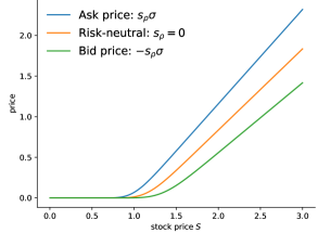
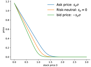
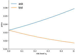
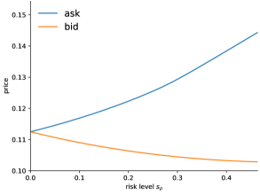
Figure 2 displays risk-averse prices for put and call options from buyer’s and seller’s perspectives. As a reference we include the risk-neutral Black–Scholes price as well. For this illustration we choose $T=1$ with strike $K=1.2$ , the interest rate is $r=3\,\%$ and the volatility is $\sigma=15\,\%$ . Figure 3 exhibits the bid-ask spread, which is present in the risk-averse situation.

4.2.3 Discussion of the risk level $s_{\rho}$

The Sharpe ratio is

\frac{\mu-r}{\sigma},

where $\mu$ is the mean return of an asset with volatility $\sigma$ and $r$ is the risk free interest rate. Comparing units in (24) we see that $s_{\rho}\,\sigma$ is an interest rate and hence $s_{\rho}$ has unit

\frac{\mathit{interest}}{\mathit{volatility}},

the same unit as the Sharpe ratio.

To explore that the risk-aversion coefficient $s_{\rho}$ has the structure of a Sharpe ratio denote by $\mu_{\mathit{averse}}$ the mean return a risk-averse investor expects. Depending on the sign we may equate

\frac{\mu_{\mathit{averse}}-r}{\sigma}=\pm s_{\rho}

(27)

with $s_{\rho}$ as in (6) above. The parallel shift

r-\mu_{\mathit{averse}}=\pm s_{\rho}\cdot\sigma

over the risk free interest derived from (27) is known as Z-spread in economics.

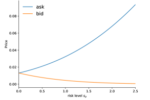
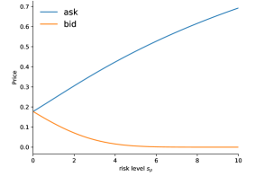
Remark 19.

Figure 3 (as well as Figure 6 below) reveals opposite slopes of the bid and ask price at $s_{\rho}=0$ , the Black–Scholes price. This reflects the opposing risk assessment of the buying and selling investor at comparable risk aversion coefficients. The value function (25) is indeed differentiable at $s_{\rho}=0$ and the sensitivity with respect to the risk dividend $s_{\rho}\,\sigma$ relates to the classical Greek $\varepsilon$ (or $\psi$ ) for dividend paying models.

4.3 Consistency with discrete models

We return to the binomial model with risk-averse probabilities from Remark 3. The preceding discussions on divisibility and the risk generator show that the risk level $\beta$ for the mean semi-deviation risk measure needs to be proportional to

\sqrt{\Delta t}.

Further recall the risk-neutral probabilities

p=\frac{e^{r\Delta t}-e^{-\sigma\sqrt{\Delta t}}}{e^{\sigma\sqrt{\Delta t}}-e^{-\sigma\sqrt{\Delta t}}}=\frac{1}{2}+\left(\frac{r}{2\sigma}-\frac{\sigma}{4}\right)\sqrt{\Delta t}+o(\Delta t)

and hence the risk-averse probabilities in (4) satisfy

\widetilde{p}=p(1-\beta\sqrt{\Delta t}(1-p))=\frac{1}{2}+\left(\frac{r-\frac{\beta\,\sigma}{2}}{2\sigma}-\frac{\sigma}{4}\right)\sqrt{\Delta t}+o(\Delta t).

Thus replacing the interest rate $r$ by $r-\frac{\beta\,\sigma}{2}$ shows that under the nested mean semi-deviation the distribution for the stock $S_{t}$ is

S_{t}=S_{0}\exp\left\{t\left(r-\frac{\beta\,\sigma}{2}-\frac{\sigma^{2}}{2}\right)+\sigma\,W_{t}\right\}.

Recall from Lemma 6 that $s_{\rho}=\frac{\beta}{\sqrt{2\pi}}$ for the mean semi-deviation of order $p=1$ . However, the binomial model converges to a process with dividends $\frac{\beta}{2}\sigma>s_{\rho}\,\sigma$ . The deviating scaling factors are in line with the discontinuity of coherent risk measures with respect to convergence in distribution, described in Bäuerle and Müller (2006, Theorem 4.1). The discussion shows that adapting the risk level $\beta$ of the nested mean semi-deviation leads to a well-defined limit in continuous time.

In general, one may not expect that nesting conditional risk measures leads to a well-defined risk measure in continuous time. Xin and Shapiro (2011) first observed that naively nesting the conditional Average Value-at-Risk leads to an exponentially increasing upper bound and Pichler and Schlotter (2019) extend this result to more general risk measures (see also Pichler (2017) for a collection of related inequalities).

The following proposition extends the discussion of the nested mean semi-deviation to more general risk measures and provides the theoretical connection between divisibility and convergence of risk-averse option pricing models.

Proposition 20.

Denote by $S^{n}$ the $n$ -period binomial tree model (3) converging to a geometric Brownian motion for $n\to\infty$ . Then the risk-averse binomial model in Remark 3 converges if the family of nested risk measures is divisible.

Proof.

Let $(\rho_{\Delta t})_{\Delta t}$ be a divisible family of risk measures and denote by $X=(X_{t})_{t}$ the geometric Brownian motion. As $X_{0}=S_{0}^{n}$ for all $n$ we have the following inequality,

\lim_{n\to\infty}\rho_{\Delta t}\left(S_{\Delta t}^{n}-S_{0}^{n}\right)\leq\lim_{n\to\infty}\rho_{\Delta t}\left(S_{\Delta t}^{n}-X_{\Delta t}\right)+\rho_{\Delta t}\left(X_{\Delta t}-X_{0}\right).

Because $(\rho_{\Delta t})_{\Delta t}$ is a divisible family of risk measures Proposition 11 shows that

\rho_{\Delta t}\left(X_{\Delta t}-X_{0}\right)=c_{\rho}\cdot\Delta t+o(\Delta t).

For the first term notice that $(S_{\Delta t}^{n}-X_{\Delta t})_{n}$ tends to zero in distribution and hence also converges in probability. Moreover, $\left(S_{\Delta t}^{n}-X_{\Delta t}\right)_{n}$ is uniformly bounded in $L^{p}$ and hence with divisibility and dominated convergence

\lim_{n\to\infty}\rho_{\Delta t}\left(S_{\Delta t}^{n}-X_{\Delta t}\right)=0.

It follows that

\lim_{n\to\infty}\rho_{\Delta t}\left(S_{\Delta t}^{n}-S_{0}^{n}\right)=c_{\rho}\cdot\Delta t+o(\Delta t),

which implies the existence of the limit of risk-averse binomial models as in Remark 3. ∎

4.4 Pricing of American options under risk

The Black–Scholes model allows explicit formulae for European option prices in in the risk-averse setting. This is surprising given the initial nonlinear PDE formulation in (22) and (23). Similarly we may reformulate the risk-averse American option pricing problem and in what follows we introduce the risk-averse optimal stopping problem for American put options and introduce the value functions.

Again we assume that the stock $S$ follows the geometric Brownian motion (19). Here, the risk-averse bid price of an American option is given by $\sup_{\tau\in[0,T]}\,-\rho^{0:\tau}\left[-e^{-r\tau}\,\Psi(S_{\tau})\right]$ , where $\Psi(\cdot)$ is the payoff function and the supremum is among all stopping times with $\tau\in[0,T]$ . The ask price is given by $\sup_{\tau\in[0,T]}\,\rho^{0:\tau}\left[e^{-r\tau}\,\Psi(S_{\tau})\right]$ . We can further define the value functions

V(t,x):=\sup_{\tau\in[t,T]}\,-\rho^{t:\tau}\left[-e^{-r(\tau-t)}\,\Psi(S_{\tau})\mid S_{t}=x\right]

for the bid price and

\widetilde{V}(t,x):=\sup_{\tau\in[t,T]}\,\rho^{t:\tau}\left[e^{-r(\tau-t)}\,\Psi(S_{\tau})\mid S_{t}=x\right]

for the ask price. For brevity we only discuss the bid price for American put options, the arguments for the ask price are analogous. By informally extending the arguments from the risk-neutral setting to the risk-averse setting we obtain the free boundary problem

$\displaystyle V_{t}(t,x)+rxV_{x}(t,x)+\frac{\sigma^{2}x^{2}}{2}V_{xx}(t,x)-s_{\rho}\sigma x\left\|V_{x}\right\|=$	$\displaystyle rV(t,x)$	$\displaystyle\text{for }x\geq L(t),$	(28)
$\displaystyle V(t,x)=$	$\displaystyle(K-x)_{+}$	$\displaystyle\text{for }0\leq x<L(t),$	(29)
$\displaystyle V_{x}(t,x)=$	$\displaystyle-1$	$\displaystyle\text{for }x=L(t),$	(30)
$\displaystyle V(T,x)=$	$\displaystyle(K-x)_{+}$
$\displaystyle L(T)=$	$\displaystyle K$
$\displaystyle\lim_{x\to\infty}V(t,x)=$	$\displaystyle 0$	$\displaystyle\text{for }0\leq t\leq T$	(31)

for the optimal exercise boundary $t\mapsto L(t)$ . For an overview on American options and free boundary problems in general we refer to Peskir and Shiryaev (2006). The following result follows with standard arguments for American options.

Theorem 21.

The value function

V(t,x)=\sup_{\tau\in[t,T]}\,-\rho^{t:\tau}\left[-e^{-r(\tau-t)}(K-S_{\tau})_{+}\mid S_{t}=x\right]

(32)

solves the free boundary problem (28)–(31).

Similarly to European options, risk-aversion reduces to a modification of the drift term and the standard American put option model applies for an underlying stock with risk dividends. To this end notice that

	$\displaystyle V_{t}(t,x)+rxV_{x}(t,x)$	$\displaystyle+\frac{\sigma^{2}x^{2}}{2}V_{xx}(t,x)-s_{\rho}\sigma x\left\|V_{x}\right\|$
	$\displaystyle=\inf_{y\in[-1,1]}$	$\displaystyle\left\{V_{t}(t,x)+\left(r-s_{\rho}\sigma y\right)xV_{x}(t,x)+\frac{\sigma^{2}x^{2}}{2}V_{xx}(t,x)\right\}$

provided that $x\geq L(t)$ . The American option is not exercised and the same arguments as for the European options show that the infimum over all constraints is attained at $y=-1$ . The equation (28) is thus equal to

V_{t}(t,x)+\left(r+s_{\rho}\sigma\right)xV_{x}(t,x)+\frac{\sigma^{2}x^{2}}{2}V_{xx}(t,x)=r\,V(t,x)\qquad\text{for }x\geq L(t).

Consequently we deduce that the value function

V(t,x):=\sup_{\tau\in[t,T]}\,\operatorname{{\mathds{E}}}\left[e^{-r(\tau-t)}\Psi\left(S_{\tau}\right)\mid S_{t}=x\right]

solves the free boundary problem (28)–(31), where the state process is given by

\displaystyle\mathrm{d}S_{s}

\displaystyle=\left(r+s_{\rho}\,\sigma\right)S_{s}\,\mathrm{d}s+\sigma\,S_{s}\,\mathrm{d}W_{s}

for a risk-loaded interest interest rate.

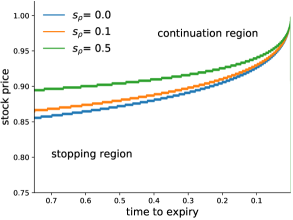
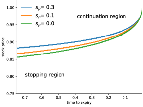
Numerical illustration

Consider the geometric Brownian motion

	$\displaystyle\mathrm{d}S_{t}$	$\displaystyle=0.03S_{t}\,\mathrm{d}t+0.15S_{t}\,\mathrm{d}W_{t},\qquad 0<t\leq 1,$
	$\displaystyle S_{0}$	$\displaystyle=1.$

The strike price in the next Figure 4 is $K=1$ . We consider the optimal stopping region for different risk levels $s_{\rho}$ . A risk-averse option buyer (bid price) would generally exercise earlier, he accepts less profits due to his risk aversion. Compared with the risk-neutral investor, the risk aware option buyer prefers exercising prematurely rather than delayed exercise.

The reverse is true for the option holder (ask price), where the investor waits longer.

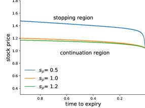
In the risk-neutral case it is never optimal to exercise an American call option before expiry. However, this is only the case if the interest rate exceeds the dividends of the underlying asset (see, for instance, Shreve (2010, Chapter 8.5) for details). As nested risk measures modify the interest rate it may be optimal to exercise the call option early. Figure 5 shows the optimal exercise boundary for the risk-averse call option with strike $K=1$ and initial value $S_{0}=1$ .

Below we show the bid-ask spread for American options.

5 The Merton problem

The preceding sections demonstrate that classical option pricing models generalize naturally to a risk-averse setting by employing nested risk measures. In what follows we demonstrate that the classical Merton problem, which allows an explicit solution in specific situations, as well allows extending to the risk-averse situation.

Consider a risk-less bond $B$ satisfying the ordinary differential equation $\mathrm{d}B_{t}=r\,B_{t}\,\mathrm{d}t$ and a risky asset $S$ driven by the stochastic differential equation

\mathrm{d}S_{t}=\mu S_{t}\,\mathrm{d}t+\sigma S_{t}\,\mathrm{d}W_{t}.

We are interested in the optimal fraction $\pi_{t}$ of the total wealth $w_{t}$ one should invest in the risky asset. The wealth process is

\mathrm{d}w_{t}=\left[\left(\pi_{t}\mu+(1-\pi_{t})r\right)w_{t}-c_{t}\right]\mathrm{d}t+\pi_{t}\,\sigma\,w_{t}\,\mathrm{d}W_{t},

where $c_{t}$ is the rate of consumption. Following Merton we employ the power utility function $u(x)=\frac{x^{1-\gamma}}{1-\gamma}$ with parameter $\gamma\geq 0$ and $\gamma\neq 1$ and consider the risk-averse objective function

R(t,x):=\sup_{\pi,c}\,-\rho^{t:T}\left(-\int_{t}^{T}u(c_{s})\mathrm{d}s-\epsilon^{\gamma}\,u(w_{T})\mid w_{t}=x\right),

(33)

where $\epsilon$ parameterizes the desired payout at terminal time. Surprisingly, $R$ has a closed form solution and the optimal portfolio allocation of the risk averse investor is

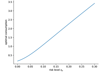
\pi^{*}=\max\left(\frac{\mu-r-s_{\rho}\,\sigma}{\sigma^{2}\,\gamma},0\right).

We observe again that risk aversion leads to a modified drift term $r+s_{\rho}\sigma$ in place of $r$ . The optimal portfolio allocation $\pi^{*}$ is a decreasing function of $s_{\rho}$ . This is in line with the usual economic perception, as increasing risk-aversion corresponds to less investments into the risky asset. The optimal consumption is given by

c_{t}^{*}(x)=\frac{x\,\nu}{1+(\nu\,\epsilon-1)e^{-\nu(T-t)}},

where $\nu$ is a constant depending on the model parameters. Consumption generally increases with risk aversion as the value of immediate consumption offsets the present value of uncertain wealth in the future.

In Remark 16 we formally extended the results of Proposition 11 to objective functions of the form (33). Based on this we now consider the Hamilton–Jacobi–Bellman equation

\displaystyle 0

\displaystyle=\max_{\pi,c}\,\left[R_{t}+\left[\left(\pi_{t}\,\mu+(1-\pi_{t})r\right)x-c_{t}\right]R_{x}+\frac{\sigma^{2}\pi^{2}x^{2}}{2}R_{xx}+u(c_{t})-s_{\rho}\left|\sigma\,\pi_{t}\,x\,R_{x}\right|\right]

(34)

with terminal condition $R(T,x)=\frac{\epsilon^{\gamma}}{1-\gamma}x^{1-\gamma}$ . In what follows we derive the optimal value function $R$ and verify the optimal portfolio allocation $\pi^{*}$ and optimal consumption $c^{*}$ given above.

The Hamilton–Jacobi–Bellman equation (34) allows for explicit optimal controls outlined in the following proposition.

Proposition 22.

In the risk-averse setting, the optimal controls are given by

\displaystyle\pi_{t}^{*}

\displaystyle(x)=-\frac{(\mu-r)R_{x}}{\sigma^{2}xR_{xx}}+\frac{s_{\rho}\sigma\left|R_{x}\right|}{\sigma^{2}xR_{xx}},\qquad c_{t}^{*}(x)=R_{x}^{-\frac{1}{\gamma}}.

The Hamilton-Jacobi-Bellman equation (34) rewrites as

	$\displaystyle 0$	$\displaystyle=R_{t}-\frac{\left((\mu-r)^{2}+s_{\rho}^{2}\sigma^{2}\right)R_{x}^{2}}{2\sigma^{2}R_{xx}}+\frac{s_{\rho}R_{x}\left\|R_{x}\right\|}{\sigma R_{xx}}+rxR_{x}+\frac{\gamma}{1-\gamma}R_{x}^{\frac{\gamma-1}{\gamma}},$		(35)
	$\displaystyle R(T,x)$	$\displaystyle=\frac{\epsilon^{\gamma}}{1-\gamma}x^{1-\gamma}.$

The preceding proposition derives first order conditions for the fraction $\pi_{t}^{*}$ and consumption rate $c_{t}^{*}$ . Employing the Hamilton–Jacobi–Bellman equations we obtain nonlinear second order partial differential equations for the optimally controlled value function.

Theorem 23 (Solution of the risk-averse Merton problem).

The PDE (35) has the explicit solution

R(t,x)=\left(\frac{1+(\nu\,\epsilon-1)e^{-\nu(T-t)}}{\nu}\right)^{\gamma}\frac{x^{1-\gamma}}{1-\gamma},

where $\nu:=-r\frac{1-\gamma}{\gamma}-\frac{1-\gamma}{\gamma^{2}}\left(\frac{\left((\mu-r)^{2}+s_{\rho}^{2}\sigma^{2}\right)}{2\sigma^{2}}-\frac{s_{\rho}}{\sigma}\right)$ . Moreover, the optimal controls are

	$\displaystyle\pi^{*}$	$\displaystyle=\max\left(\frac{(\mu-r)-s_{\rho}\sigma}{\sigma^{2}\gamma},0\right)\text{ and}$
	$\displaystyle c_{t}^{*}(x)$	$\displaystyle=\frac{x\,\nu}{1+(\nu\,\epsilon-1)e^{-\nu(T-t)}}.$

Proof.

We recall the PDE (35),

	$\displaystyle 0$	$\displaystyle=R_{t}-\frac{\left((\mu-r)^{2}+s_{\rho}^{2}\sigma^{2}\right)R_{x}^{2}}{2\sigma^{2}R_{xx}}+\frac{s_{\rho}R_{x}\left\|R_{x}\right\|}{\sigma R_{xx}}+rxR_{x}+\frac{\gamma}{1-\gamma}\left(R_{x}\right)^{\frac{\gamma-1}{\gamma}},$
	$\displaystyle R(T,x)$	$\displaystyle=\epsilon^{\gamma}\frac{x^{1-\gamma}}{1-\gamma},$

and choose the ansatz $R(t,x)=f(t)^{\gamma}\frac{x^{1-\gamma}}{1-\gamma}$ . In this case the partial derivatives are given by

	$\displaystyle R_{t}$	$\displaystyle=\left(\gamma f(t)^{\gamma-1}f^{\prime}(t)\right)\frac{x^{1-\gamma}}{1-\gamma},$
	$\displaystyle R_{x}$	$\displaystyle=f(t)^{\gamma}x^{-\gamma},$
	$\displaystyle R_{xx}$	$\displaystyle=-\gamma f(t)^{\gamma}x^{-\gamma-1}.$

The terminal condition for our Merton problem is $R(T,x)=\epsilon^{\gamma}\frac{x^{1-\gamma}}{1-\gamma}$ hence $f(T)=\epsilon>0$ . Setting $C_{1}:=-\frac{\left((\mu-r)^{2}+s_{\rho}^{2}\sigma^{2}\right)}{2\sigma^{2}}$ and $C_{2}:=\frac{s_{\rho}}{\sigma}$ for ease of notation we substitute the derivatives in the PDE (35) and obtain the following ordinary differential equation for $f$ ;

\displaystyle f^{\prime}(t)

\displaystyle=f(t)\left(-r\frac{1-\gamma}{\gamma}+\frac{1-\gamma}{\gamma^{2}}\left(C_{1}+C_{2}f^{\gamma}\right)\right)-1.

(36)

For $\nu$ as defined in Theorem 23, the general solution of the ordinary differential equation (36) is

f(t)=\frac{1+(\nu\epsilon-1)e^{-\nu(T-t)}}{\nu},

which is positive. The optimal value function thus is

\displaystyle R(t,x)

\displaystyle=\left(\frac{1+(\nu\epsilon-1)e^{-\nu(T-t)}}{\nu}\right)^{\gamma}\frac{x^{1-\gamma}}{1-\gamma}.

It follows that the the optimal control is $\pi_{t}^{*}=\max\left(\frac{(\mu-r)-s_{\rho}\sigma}{\sigma^{2}\gamma},0\right)$ , where the optimal consumption process is $c_{t}^{*}=\frac{x\nu}{1+(\nu\epsilon-1)e^{-\nu(T-t)}},$ which concludes the proof. ∎

The following Figure 7 illustrates the optimal consumption $c^{*}$ as a function of the risk level $s_{\rho}$ for $\gamma=0.4$ , $r=0.01$ , $\mu=0.1$ , $\sigma=0.3$ and $\epsilon=0.1$ . The time horizon is $T=4$ and we consider the wealth $w_{0}=1$ . Note that $s_{\rho}$ can take only values smaller than $\frac{\mu-r}{\sigma}$ as otherwise $\pi^{*}<0$ .

6 Summary

This paper introduces risk aversion in classical models of finance by introducing nested risk measures. We demonstrate that classical formulae, which are of outstanding importance in economics, are explicitly available in the risk-averse setting as well. This includes the binomial option pricing model, the Black–Scholes model as well as Merton’s optimal consumption problem.

We give an explicit Z-spread, which reflects the degree of risk aversion. The Z-spread involves the volatility of the risky asset and a constant, which indicates risk aversion. The results thus provide an economic interpretation of the Z-spread by thorough risk management by iterating risk measures.

We extend nested risk measures from a discrete time to a continuous time setting. This allows deriving a non-linear risk generator expressing the momentary dynamics of the classical model under risk aversion. We demonstrate that the risk generator has a unique structure for all coherent risk measures up to the constant, the coefficient of risk aversion. The risk aversion constant is also naturally associated with the Sharpe ratio.

Acknowledgment

We thank two anonymous referees for many insightful comments and helpful discussions on this topic.

References

Artzner et al. (1999) P. Artzner, F. Delbaen, J.-M. Eber, and D. Heath. Coherent Measures of Risk. Mathematical Finance, 9:203–228, 1999. doi:10.1111/1467-9965.00068.
Barles and Soner (1998) G. Barles and H. Soner. Option pricing with transaction costs and a nonlinear black-scholes equation. Finance and Stochastics, 2, 1998. doi:10.1007/s007800050046.
Bäuerle and Müller (2006) N. Bäuerle and A. Müller. Stochastic orders and risk measures: Consistency and bounds. Insurance: Mathematics and Economics, 38(1):132–148, 2006. doi:10.1016/j.insmatheco.2005.08.003.
Cheridito et al. (2004) P. Cheridito, F. Delbaen, and M. Kupper. Coherent and convex monetary risk measures for bounded càdlàg processes. Stochastic Processes and their Applications, 112(1):1–22, jul 2004. doi:10.1016/j.spa.2004.01.009.
Cheridito et al. (2006) P. Cheridito, F. Delbaen, and M. Kupper. Dynamic monetary risk measures for bounded discrete-time processes. Electronic Journal of Probability, (3):57–106, 2006. ISSN 1083-6489. doi:10.1214/EJP.v11-302.
De Lara and Leclère (2016) M. De Lara and V. Leclère. Building up time-consistency for risk measures and dynamic optimization. European Journal of Operational Research, 249:177–187, 2016. doi:10.1016/j.ejor.2015.03.046.
Delbaen (2002) F. Delbaen. Coherent risk measures on general probability spaces. In Essays in Honour of Dieter Sondermann, pages 1–37. Springer-Verlag, Berlin, 2002.
Delbaen and Schachermayer (2006) F. Delbaen and W. Schachermayer. The Mathematics of Arbitrage. Springer, 2006.
Delong (2013) L. Delong. Backwards Stochastic Differential Equations with Jumps and Their Actuarial and Financial Applications. 2013. ISBN 978-1-4471-5330-6. doi:10.1007/978-1-4471-5331-3.
Fleming and Soner (2006) W. H. Fleming and H. Soner. Controlled Markov Processes and Viscosity Solutions. 2006. ISBN 0-387-26045-5.
Garman and Kohlhagen (1983) M. B. Garman and S. W. Kohlhagen. Foreign currency option values. Journal of International Money and Finance, 2:231–237, 1983. doi:10.1016/s0261-5606(83)80001-1.
Guigues and Römisch (2012) V. Guigues and W. Römisch. Sampling-based decomposition methods for multistage stochastic programs based on extended polyhedral risk measures. SIAM Journal on Optimization, 22(2):286–312, jan 2012. doi:10.1137/100811696.
Karatzas and Shreve (1998) I. Karatzas and S. E. Shreve. Methods of Mathematical Finance. Springer New York, 1998. doi:10.1007/978-1-4939-6845-9.
Klenke (2014) A. Klenke. Probability Theory. Springer London, 2014. doi:10.1007/978-1-4471-5361-0.
Maggioni et al. (2012) F. Maggioni, E. Allevi, and M. Bertocchi. Bounds in multistage linear stochastic programming. Journal of Optimization Theory and Applications, 163(1):200–229, 2012. doi:10.1007/s10957-013-0450-1.
Merton (1973) R. C. Merton. Theory of rational option pricing. The Bell Journal of Economics and Management Science, 4(1):141–183, 1973.
Øksendal (2003) B. Øksendal. Stochastic Differential Equations. Springer Berlin Heidelberg, 2003. doi:10.1007/978-3-642-14394-6.
Pardoux and Peng (1990) E. Pardoux and S. Peng. Adapted solution of a backward stochastic differential equation. Systems & Control Letters, 14(1):55–61, 1990. doi:10.1016/0167-6911(90)90082-6.
Peng (2004) S. Peng. Nonlinear Expectations, Nonlinear Evaluations and Risk Measures. Springer, Berlin, Heidelberg, 2004. doi:10.1007/978-3-540-44644-6_4.
Peskir and Shiryaev (2006) G. Peskir and A. Shiryaev. Optimal Stopping and Free-Boundary Problems. Birkhäuser Basel, 2006. doi:10.1007/978-3-7643-7390-0.
Pflug and Römisch (2007) G. Ch. Pflug and W. Römisch. Modeling, Measuring and Managing Risk. World Scientific, 2007. doi:10.1142/9789812708724.
Philpott et al. (2013) A. Philpott, V. de Matos, and E. Finardi. On solving multistage stochastic programs with coherent risk measures. Operations Research, 61(4):957–970, aug 2013. doi:10.1287/opre.2013.1175.
Philpott and de Matos (2012) A. B. Philpott and V. L. de Matos. Dynamic sampling algorithms for multi-stage stochastic programs with risk aversion. European Journal of Operational Research, 218(2):470–483, 2012. doi:10.1016/j.ejor.2011.10.056.
Pichler (2017) A. Pichler. A quantitative comparison of risk measures. Annals of Operations Research, 2017. doi:10.1007/s10479-017-2397-3.
Pichler and Schlotter (2019) A. Pichler and R. Schlotter. Martingale characterizations of risk-averse stochastic optimization problems. Mathematical Programming, 181(2):377–403, 2019. doi:10.1007/s10107-019-01391-2.
Riedel (2004) F. Riedel. Dynamic coherent risk measures. Stochastic Processes and their Applications, 112(2):185–200, 2004. doi:10.1016/j.spa.2004.03.004.
Ruszczyński and Shapiro (2006) A. Ruszczyński and A. Shapiro. Conditional risk mappings. Mathematics of Operations Research, 31(3):544–561, 2006. doi:10.1287/moor.1060.0204.
Ruszczyński and Yao (2015) A. Ruszczyński and J. Yao. A risk-averse analogue of the Hamilton–Jacobi–Bellman equation. In Proceedings of the Conference on Control and its Applications, chapter 62, pages 462–468. Society for Industrial and Applied Mathematics (SIAM), 2015. doi:10.1137/1.9781611974072.63.
Ševčovič and Žitňanská (2016) D. Ševčovič and M. Žitňanská. Analysis of the nonlinear option pricing model under variable transaction costs. Asia-Pacific Financial Markets, 23(2):153–174, mar 2016. doi:10.1007/s10690-016-9213-y.
Shapiro et al. (2014) A. Shapiro, D. Dentcheva, and A. Ruszczyński. Lectures on Stochastic Programming: Modeling and Theory. 2nd edition, 2014. doi:10.1137/1.9780898718751.
Shreve (2010) S. E. Shreve. Stochastic Calculus for Finance II. Springer New York, 2010. ISBN 0387401016. URL https://www.ebook.de/de/product/2835534/steven_e_shreve_stochastic_calculus_for_finance_ii.html.
Stadje (2010) M. Stadje. Extending dynamic convex risk measures from discrete time to continuous time: A convergence approach. Insurance: Mathematics and Economics, 47(3):391–404, dec 2010. doi:10.1016/j.insmatheco.2010.08.005.
Xin and Shapiro (2011) L. Xin and A. Shapiro. Bounds for nested law invariant coherent risk measures. Operation Research Letters, 2011. doi:10.1016/j.orl.2012.09.002.

Appendix A A sufficient condition for Hölder continuity

We give a sufficient condition for the Hölder continuity property (11) in Proposition 11.

Proposition 24.

Let $X$ be a solution of the stochastic differential equation (9) where the drift $b$ and the diffusion $\sigma$ satisfy the usual conditions of Øksendal (2003, Theorem 5.2.1). Furthermore suppose that for a fixed $p>2$ the moments $\operatorname{{\mathds{E}}}X_{t}^{p}$ are finite for every $t\in\mathcal{T}$ and that the diffusion coefficient satisfies

\left|\sigma(t,x)-\sigma(s,x)\right|\leq\widetilde{D}\left|t-s\right|^{\alpha},\hfill\text{for all }x\in\mathbb{R}

for some $\gamma\in(0,\nicefrac{{1}}{{2}})$ . Then the Assumption (11) is satisfied, i.e., $\operatorname{{\mathds{E}}}C^{p}<\infty$ and in particular there exists a constant such that

\operatorname{{\mathds{E}}}C^{p}<C(\alpha,p,\mathcal{T},\widetilde{D}).

Proof.

First observe that the usual conditions of Øksendal (2003, Theorem 5.2.1) as well as the assumption in Proposition 24 ensures that there exist $D,\widetilde{D}\in\mathbb{R}$ such that

	$\displaystyle\left\|\sigma(t,X_{t})-\sigma(s,X_{s})\right\|$	$\displaystyle\leq\left\|\sigma(t,X_{t})-\sigma(t,X_{s})\right\|+\left\|\sigma(t,X_{s})-\sigma(s,X_{s})\right\|$
		$\displaystyle\leq D\left\|X_{t}-X_{s}\right\|+\widetilde{D}\left\|t-s\right\|.$

Therefore consider Hölder bounds on $\left|X_{t}-X_{s}\right|$ , let $p>2$ and recall the estimate

(a+b)^{p}\leq 2^{p}(a^{p}+b^{p}),\qquad a,b\geq 0

which implies

|X_{u}|^{p}\leq 2^{p}\left|\int_{0}^{u}b(v,X_{v})\,\mathrm{d}v\right|^{p}+2^{p}\left|\int_{0}^{u}\sigma(v,X_{v})\,\mathrm{d}W_{v}\right|^{p}.

Estimate the terms separately and consider the first term. Jensen’s inequality applied to the probability measure $\frac{\mathrm{d}v}{u}$ shows

	$\displaystyle\left\|\int_{0}^{u}b(v,X_{v})\,\mathrm{d}v\right\|^{p}$	$\displaystyle=u^{p}\left\|\int_{0}^{u}b(v,X_{v})\,\frac{\mathrm{d}v}{u}\right\|^{p}$
		$\displaystyle\leq u^{p-1}\int_{0}^{u}\|b(v,X_{v})\|^{p}\,\mathrm{d}v$
		$\displaystyle\leq C^{p}u^{p-1}\int_{0}^{u}(1+\|X_{v}\|)^{p}\,\mathrm{d}v$
		$\displaystyle\leq 2^{p}C^{p}u^{p-1}(u+\int_{0}^{u}\|X_{v}\|^{p}\,\mathrm{d}v).$

To estimate the second term use the Burkholder-Davis-Gundy inequality

	$\displaystyle\operatorname{{\mathds{E}}}\left\|\int_{0}^{u}\sigma(v,X_{v})\,\mathrm{d}W_{v}\right\|^{p}$	$\displaystyle\leq c(p)\operatorname{{\mathds{E}}}\left(\int_{0}^{u}\|\sigma(v,X_{v})\|^{2}\,\mathrm{d}v\right)^{\nicefrac{{p}}{{2}}}$
		$\displaystyle\leq c(p)\operatorname{{\mathds{E}}}\left[u^{\nicefrac{{p}}{{2}}-1}\int_{0}^{u}\left\|\sigma(v,X_{v})\right\|^{p}\,\mathrm{d}v\right]$
		$\displaystyle\leq c(p)C^{p}u^{\nicefrac{{p}}{{2}}-1}\operatorname{{\mathds{E}}}\int_{0}^{u}(1+\left\|X_{v}\right\|)^{p}\,\mathrm{d}v$
		$\displaystyle\leq c(p)(2C)^{p}u^{\nicefrac{{p}}{{2}}-1}(u+\int_{0}^{u}\operatorname{{\mathds{E}}}\left\|X_{v}\right\|^{p}\,\mathrm{d}v).$

An application of Gronwall’s lemma for both terms provides upper bounds

\operatorname{{\mathds{E}}}\left|\int_{s}^{t}b(v,X_{v})\,\mathrm{d}v\right|^{p}\leq C_{\text{Gronwall}}(C,p,t)(t-s)^{p}

and

\operatorname{{\mathds{E}}}\left|\int_{s}^{t}\sigma(v,X_{v})\,\mathrm{d}W_{v}\right|^{p}\leq\widetilde{C}_{\text{Gronwall}}(C,p,t)(t-s)^{\frac{p}{2}}.

It follows by adding up and choosing an appropriate constant $C^{*}$ that for $|t-s|<1$

\operatorname{{\mathds{E}}}\left|X_{t}-X_{s}\right|^{p}\leq C^{*}(t-s)^{\frac{p}{2}}.

As $p>2$ we can identify $\frac{p}{2}=1+\beta$ for some $\beta>0$ which shows that the assumptions of Kolmogorovs continuity theorem (cf. Theorem 21.6 in Klenke (2014)) are satisfied and implying that there exists a random $C_{r}>0$ such that

\left|X_{t}-X_{s}\right|\leq C_{r}\left|t-s\right|^{\alpha}

(37)

for $\alpha\in(0,\frac{\beta}{p})$ .

It remains to show that the $p$ -norm of $C_{r}$ in (37) can be bounded. To show this, recall the Garsia–Rodemich–Rumsey inequality. For any $p>1$ and $\delta>\frac{1}{p}$ , there is a constant $C(\delta,p)\in\mathbb{R}$ such that for any $f\in C([0,T],\mathbb{R})$ and $t,s\in[0,T]$

\left|f(t)-f(s)\right|^{p}\leq C(\delta,p)|t-s|^{\delta p-1}\int_{s}^{t}\int_{s}^{t}\frac{\left|f(u)-f(v)\right|^{p}}{|u-v|^{\delta p+1}}\,\mathrm{d}u\,\mathrm{d}v.

It suffices to consider $C_{r}:=||X||_{\alpha;[0,T]}$ , the Hölder norm of $X$ defined by

||X||_{\alpha;[0,T]}:=\sup_{0\leq t<s\leq T}\frac{\left|X_{t}-X_{s}\right|}{|t-s|^{\alpha}}.

For any $0<\alpha<\frac{\beta}{p}$ take $\delta\in\left(\frac{1}{p},\alpha+\frac{1}{p}\right)$ to get

	$\displaystyle\operatorname{{\mathds{E}}}\left[\|\|X\|\|_{\alpha;[0,T]}^{p}\right]$	$\displaystyle\leq C(\delta,p)\int_{0}^{T}\int_{0}^{T}\frac{\operatorname{{\mathds{E}}}\left[\left\|X_{t}-X_{s}\right\|^{p}\right]}{\|u-v\|^{\delta p+1}}\,\mathrm{d}u\,\mathrm{d}v$
		$\displaystyle\leq C(\delta,p)C^{*}\int_{0}^{T}\int_{0}^{T}\frac{\left\|t-s\right\|^{1+\beta}}{\|u-v\|^{\delta p+1}}\,\mathrm{d}u\,\mathrm{d}v$
		$\displaystyle=C(\delta,p)C^{*}\int_{0}^{T}\int_{0}^{T}\|u-v\|^{\beta-\delta p}\,\mathrm{d}u\,\mathrm{d}v$
		$\displaystyle=C(\delta,p,T)C^{*}.$

Here the second inequality follows from the first step. We conclude the assertion by observing that

	$\displaystyle\left\|\sigma(t,X_{t})-\sigma(s,X_{s})\right\|$	$\displaystyle\leq D\left\|X_{t}-X_{s}\right\|+\left\|\sigma(t,X_{s})-\sigma(s,X_{s})\right\|$
		$\displaystyle\leq DC_{r}\left\|t-s\right\|^{\alpha}+\widetilde{D}\left\|t-s\right\|^{\alpha}$
		$\displaystyle=(DC_{r}+\widetilde{D})\left\|t-s\right\|^{\alpha},$

where the constant $DC_{r}+\widetilde{D}$ is $p$ -integrable. ∎

	$\displaystyle\left\|\int_{0}^{u}b(v,X_{v})\,\mathrm{d}v\right\|^{p}$	$\displaystyle=u^{p}\left\|\int_{0}^{u}b(v,X_{v})\,\frac{\mathrm{d}v}{u}\right\|^{p}$
		$\displaystyle\leq u^{p-1}\int_{0}^{u}\|b(v,X_{v})\|^{p}\,\mathrm{d}v$
		$\displaystyle\leq C^{p}u^{p-1}\int_{0}^{u}(1+\|X_{v}\|)^{p}\,\mathrm{d}v$
		$\displaystyle\leq 2^{p}C^{p}u^{p-1}(u+\int_{0}^{u}\|X_{v}\|^{p}\,\mathrm{d}v).$

	$\displaystyle\operatorname{{\mathds{E}}}\left\|\int_{0}^{u}\sigma(v,X_{v})\,\mathrm{d}W_{v}\right\|^{p}$	$\displaystyle\leq c(p)\operatorname{{\mathds{E}}}\left(\int_{0}^{u}\|\sigma(v,X_{v})\|^{2}\,\mathrm{d}v\right)^{\nicefrac{{p}}{{2}}}$
		$\displaystyle\leq c(p)\operatorname{{\mathds{E}}}\left[u^{\nicefrac{{p}}{{2}}-1}\int_{0}^{u}\left\|\sigma(v,X_{v})\right\|^{p}\,\mathrm{d}v\right]$
		$\displaystyle\leq c(p)C^{p}u^{\nicefrac{{p}}{{2}}-1}\operatorname{{\mathds{E}}}\int_{0}^{u}(1+\left\|X_{v}\right\|)^{p}\,\mathrm{d}v$
		$\displaystyle\leq c(p)(2C)^{p}u^{\nicefrac{{p}}{{2}}-1}(u+\int_{0}^{u}\operatorname{{\mathds{E}}}\left\|X_{v}\right\|^{p}\,\mathrm{d}v).$

	$\displaystyle\operatorname{{\mathds{E}}}\left[\|\|X\|\|_{\alpha;[0,T]}^{p}\right]$	$\displaystyle\leq C(\delta,p)\int_{0}^{T}\int_{0}^{T}\frac{\operatorname{{\mathds{E}}}\left[\left\|X_{t}-X_{s}\right\|^{p}\right]}{\|u-v\|^{\delta p+1}}\,\mathrm{d}u\,\mathrm{d}v$
		$\displaystyle\leq C(\delta,p)C^{*}\int_{0}^{T}\int_{0}^{T}\frac{\left\|t-s\right\|^{1+\beta}}{\|u-v\|^{\delta p+1}}\,\mathrm{d}u\,\mathrm{d}v$
		$\displaystyle=C(\delta,p)C^{*}\int_{0}^{T}\int_{0}^{T}\|u-v\|^{\beta-\delta p}\,\mathrm{d}u\,\mathrm{d}v$
		$\displaystyle=C(\delta,p,T)C^{*}.$

	$\displaystyle\left\|\sigma(t,X_{t})-\sigma(s,X_{s})\right\|$	$\displaystyle\leq D\left\|X_{t}-X_{s}\right\|+\left\|\sigma(t,X_{s})-\sigma(s,X_{s})\right\|$
		$\displaystyle\leq DC_{r}\left\|t-s\right\|^{\alpha}+\widetilde{D}\left\|t-s\right\|^{\alpha}$
		$\displaystyle=(DC_{r}+\widetilde{D})\left\|t-s\right\|^{\alpha},$

Quantification of Risk in Classical Models of Finance

Abstract

1 Introduction

2 Preliminaries on risk measures

2.1 Nested risk measures

Definition 1 (Nested risk measures).

2.2 Nested risk measures for discrete processes

Definition 2 (Semi-deviation).

The binomial model.

Remark 3 (The mean semi-deviation for the binomial model).

3 The risk-averse limit of discrete option pricing models

Definition 4 (Divisible families of risk measures).

Remark 5.

Lemma 6.

Proof.

Definition 7 (Nested risk measures).

Proposition 8 (Nested mean semi-deviation for the Wiener process).

Proof.

Remark 9.

3.1 The risk generator

Definition 10 (Risk generator).

Proposition 11 (Risk generator).

Remark 12.

Proof.

Remark 13 (Relation to gg-expectation).

3.2 Dynamic programming

Lemma 14 (Dynamic programming principle).

Proof.

Theorem 15.

Proof.

Remark 16 (Optimal controls).

4 Pricing of options under risk

4.1 The risk-averse Black–Scholes model for European options

Proposition 17 (Call option).

Proposition 18 (European Put option).

Proof.

4.2 Rationale of risk aversion in the new formulae

4.2.1 On the nature of the risk level sρs_{\rho}

4.2.2 Illustration of the risk level sρs_{\rho}

4.2.3 Discussion of the risk level sρs_{\rho}

Remark 19.

4.3 Consistency with discrete models

Proposition 20.

Proof.

4.4 Pricing of American options under risk

Theorem 21.

Numerical illustration

5 The Merton problem

Proposition 22.

Theorem 23 (Solution of the risk-averse Merton problem).

Proof.

6 Summary

Acknowledgment

References

Appendix A A sufficient condition for Hölder continuity

Proposition 24.

Proof.

Remark 13 (Relation to $g$ -expectation).

4.2.1 On the nature of the risk level $s_{\rho}$

4.2.2 Illustration of the risk level $s_{\rho}$

4.2.3 Discussion of the risk level $s_{\rho}$