Quantifying structural uncertainty in the BHR model for variable-density flows

For the Reynolds decompositions of $\rho=\overline{\rho}+\rho^{\prime}$, $u_{i}=\overline{u_{i}}+u_{i}^{\prime}$ and $p=\overline{p}+p^{\prime}$ for density, velocity, and pressure, respectively, where the over-bar denotes the uniformly weighted ensemble. However, for variable-density flows, a mass-weighted averaging called Favre decomposition is employed

$$u_{i}=\widetilde{u_{i}}+u_{i}^{\prime\prime},$$

(1)

where $\widetilde{u_{i}}=\overline{\rho u_{i}}/\overline{\rho}$ and $u_{i}^{\prime\prime}$ represents the mass-weighted fluctuation with $\overline{\rho u_{i}^{\prime\prime}}=0$. Then, the mass-weighted average velocity $\widetilde{u_{i}}$ can be rewritten by applying the Reynolds decomposition

$$\tilde{u_{i}}=\frac{\overline{\rho u_{i}}}{\overline{\rho}}=\overline{u_{i}}+\frac{\overline{\rho^{\prime}u_{i}^{\prime}}}{\overline{\rho}},$$

(2)

where $\overline{\rho^{\prime}u_{i}^{\prime}}/\overline{\rho}$ is the turbulent mass-flux velocity, which is usually denoted as $a_{i}$ . Another important quantity in the BHR model equations is the density self-correlation, $b$, defined as

$$b=-\overline{\rho^{\prime}\left(\frac{1}{\rho}\right)^{\prime}},$$

(3)

which can also be written as $b=\overline{\rho^{\prime 2}/\rho\overline{\rho}}$. The generalized Reynolds stress tensor, $R_{ij}=\overline{\rho u_{i}^{\prime\prime}u_{j}^{\prime\prime}}$, is obtained by Favre decomposition.

The resulting modeled governing equations are given by

$$\frac{\partial\overline{\rho}}{\partial t}+\frac{\partial\overline{\rho}\widetilde{u_{j}}}{\partial x_{j}}=0,$$

(4)

$$\frac{\partial\overline{\rho}\widetilde{c}_{\alpha}}{\partial t}+\frac{\partial\overline{\rho}\widetilde{u_{j}}\widetilde{c}_{\alpha}}{\partial x_{j}}=\frac{\partial}{\partial x_{j}}\left(\frac{\mu_{T}\partial\widetilde{c}_{\alpha}}{\sigma_{c}\partial x_{j}}\right),$$

(5)

$$\frac{\partial\overline{\rho}\widetilde{u_{i}}}{\partial t}+\frac{\partial\overline{\rho}\widetilde{u_{j}}\widetilde{u_{i}}}{\partial x_{j}}=-\frac{\partial(\overline{p}\delta_{ij}+R_{ij})}{\partial x_{j}}+\overline{\rho}g_{i},$$

(6)

$$\frac{\partial\overline{\rho}k}{\partial t}+\frac{\partial\overline{\rho}k\widetilde{u_{i}}}{\partial x_{j}}=a_{j}\frac{\partial\overline{p}}{\partial x_{j}}-R_{ij}\frac{\partial\widetilde{u_{i}}}{\partial x_{j}}+\frac{\partial}{\partial x_{j}}\left(\frac{\mu_{T}\partial k}{\sigma_{k}\partial x_{j}}\right)-\overline{\rho}\frac{k^{3/2}}{S},$$

(7)

$$\begin{split}\frac{\partial\overline{\rho}S}{\partial t}+\frac{\partial\overline{\rho}S\widetilde{u_{i}}}{\partial x_{j}}=&\frac{S}{k}\left[\left(\frac{3}{2}-C_{4}\right)a_{j}\frac{\partial\overline{p}}{\partial x_{j}}-\left(\frac{3}{2}-C_{1}\right)R_{ij}\frac{\partial\widetilde{u_{i}}}{\partial x_{j}}\right]\\ &+\frac{\partial}{\partial x_{j}}\left(\frac{\mu_{T}\partial S}{\sigma_{S}\partial x_{j}}\right)-\left(\frac{3}{2}-C_{2}\right)\overline{\rho}k^{1/2},\end{split}$$

(8)

$$\begin{split}\frac{\partial\overline{\rho}{a_{i}}}{\partial t}+\frac{\partial\overline{\rho}\widetilde{u_{j}}{a_{i}}}{\partial x_{j}}=&b\frac{\partial\overline{p}}{\partial x_{i}}-\overline{\rho}a_{j}\frac{\partial(\widetilde{u_{i}}-a_{i})}{\partial x_{j}}-\frac{R_{ij}}{\overline{\rho}}\frac{\partial\overline{\rho}}{\partial x_{j}}\\ &+\overline{\rho}\frac{\partial a_{i}a_{j}}{\partial x_{j}}+\frac{\partial}{\partial x_{j}}\left(\frac{\mu_{T}\partial a_{i}}{\sigma_{a}\partial x_{j}}\right)-C_{a}\overline{\rho}a_{i}\frac{k^{1/2}}{S},\end{split}$$

(9)

$$b=\frac{\alpha_{1}\alpha_{2}\left(\rho_{1}-\rho_{2}\right)}{\rho_{1}\rho_{2}}.$$

(10)

where $c_{\alpha}$ is the mass fraction, $\mu_{T}$ is the turbulent eddy viscosity and is modeled as $\mu_{T}=C_{\mu}\overline{\rho}Sk^{1/2}$, $R_{ij}=2/3\overline{\rho}k\delta_{ij}-2\mu_{T}S_{ij}$ is the generalized Reynolds stress with the rate of mean strain definition $S_{ij}=1/2\left[{\partial\widetilde{u_{i}}}/{\partial x_{j}}+{\partial\widetilde{u_{j}}}/{\partial x_{i}}-{2}/{3}{\partial\widetilde{u_{k}}}/{\partial x_{k}}\delta_{ij}\right]$, $k$ is the turbulent kinetic energy, $S$ is the turbulent mixing length, and $a_{i}$ and $b$ are the turbulent mass-flux velocity and the density self-correlation, respectively, as discussed above. The averaged density $\overline{\rho}=\alpha_{1}\rho_{1}+\alpha_{2}\rho_{2}$, and $\alpha_{1}+\alpha_{2}=1$. According to previous studies (Schwarzkopf et al., 2011, 2016), the first two terms $G$ and $P$ in the right handside of turbulent kinetic energy transport equation, are the production, where $G=a_{j}{\partial\overline{p}}/{\partial x_{j}}=\mathbb{a}\cdot\mathbb{p}_{g}$ where $\mathbb{a}$ is the turbulent mass-flux velocity vector and $\mathbb{p}_{g}$ is the pressure gradient, and $P=-R_{ij}{\partial\widetilde{u_{i}}}/{\partial x_{j}}$.

The methodology to perturb the eigenvectors of the Reynolds stress tensor in the RANS modeling framework without using any additional data or modeling assumptions has been proposed (Gorlé & Iaccarino, 2013) and developed for many engineering flows (Emory et al., 2013; Gorlé et al., 2015; Mishra & Iaccarino, 2016, 2017; Thompson et al., 2019). The structural uncertainty framework works very well for many flows with separations and enables us to account for the discrepancy between experimental observations and high-fidelity simulations. The basic methodology is described as follows. The turbulence anisotropy tensor is

$$a_{ij}=\frac{R_{ij}}{2\overline{\rho}k}-\frac{1}{3}\delta_{ij},$$

(11)

The condition of realizability and the Cauchy-Schwartz inequality require that $-1/3\leq a_{ij}\leq 2/3$ for $i=j$ and $-1/2\leq a_{ij}\leq 1/2$ for $i\neq j$. The anisotropy tensor can be represented by an eigenvalue decomposition

$$a_{ij}=v_{in}\Lambda_{nl}v_{lj},$$

(12)

where $v$ denotes the eigenvector matrix and $\Lambda$ denotes the eigenvalues, and they are ordered by $\lambda_{1}\geq\lambda_{2}\geq\lambda_{3}$ without any loss of generality. Therefore, the Reynolds stress can be expressed as

$$R_{ij}=2\overline{\rho}k\left(v_{in}\Lambda_{nl}v_{lj}+\frac{1}{3}\delta_{ij}\right),$$

(13)

Perturbing the eigenvalues and eigenvector by injecting the uncertainties, one obtains the perturbed Reynolds stress.

$$R_{ij}=2\overline{\rho}k\left(v_{in}^{*}\Lambda_{nl}^{*}v_{lj}^{*}+\frac{1}{3}\delta_{ij}\right),$$

(14)

The purpose of this investigation is to develop a framework to identify and quantify the uncertainties of the BHR model for variable-density flows. For eigenspace perturbation in Reynolds stress, the states of maximizing and minimizing the production mechanism are very important. Similarly, we propose a perturbation strategy to estimate the maximal and minimal states of the production to quantify the structural uncertainty in the BHR model for variable-density flows. Note that the term $G$ in the production is the inner product of the turbulent mass-flux velocity vector and mean pressure gradient; the alignment of the two vectors gives the maximum and minimum. Recalling the maximal and minimal states of $P$ arising from the eigenspace perturbation, we can capture the maximal and minimal states of the term $P$ in the BHR model. Therefore, we can predict the model structural uncertainty intervals quantified by the production mechanism.

By perturbing the orientation of $\mathbb{a}$, i.e., the angle between the $\mathbb{a}$ and $\mathbb{p}_{g}$, the extreme states of $G$ are very easily obtained as $G_{0}$ and $G_{\pi}$, which correspond to the angle between the two vectors, $0$ and $\pi$, respectively. Perturbing the eigenvalue and eigenvectors in $P$ gives the five extreme states. By combining them, one can quantify the extreme states of the production in the BHR model by the combination of $G$ and $P$ perturbation, i.e., with the 10 states.

The BHR model, the eigenspace perturbation method, and the perturbation of $G$ are implemented in OpenFOAM to simulate variable-density flows. In this brief, we investigate three variable-density flows: 1DRT, two-dimensional Rayleigh-Taylor-driven mixing in a TR (2DTR), and turbulent jet mixing.

We first consider the 1DRT case at a low Atwood number, $At=0.04$, due to the available air-helium gas channel experimental measurements (Banerjee et al., 2010) and numerical simulations (Banerjee et al., 2010). Furthermore, the turbulent mass-flux velocity and pressure gradient have the same direction due to the 1D setup. Therefore, $G$ is certainty, and no perturbation is needed. The production perturbation is simplified to the eigenspace perturbation (Emory et al., 2013; Iaccarino et al., 2017) in the term of $P$ with the five extreme cases.

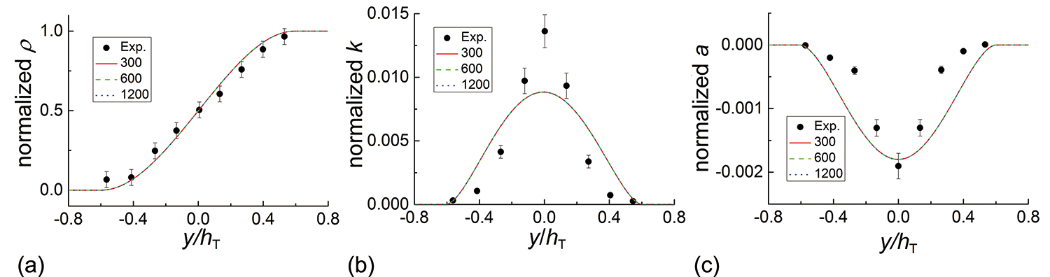
In the experiment by Banerjee et al. (2010), two gas streams, one containing air and the other containing a helium-air mixture, flow in parallel with each other separated by a thin splitter plate. The two streams meet at the end of the splitter plate, leading to the formation of an unstable interface and of buoyancy-driven mixing. The buoyancy-driven mixing experiment allows for long data collection time and is statistically steady. The experimental setup allows 1D mixing simulations at the streamwise section. The two fluids have constant densities, $\rho_{1}=$ 1.0833 g/cm³ and $\rho_{2}=$ 1.0 g/cm³, to match the experiment. The buoyancy force is relatively weak at this low Atwood number since it represents the effect of density difference on the flow mixture. The numerical results obtained with three different grid sizes are shown in Figure 1 for normalized density, turbulent kinetic energy, and turbulent mass-flux velocity. The density distribution agrees very well with the experimental data (Banerjee et al., 2010), and both the turbulent kinetic energy and mass-flux velocity show reasonable agreement. Furthermore, good grid convergence is obtained since the lines are on top of each other. Therefore, the following simulations with perturbations are performed using the $600$ grid size.

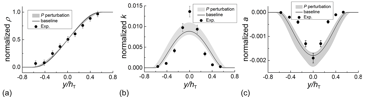
Eigenspace perturbation in Reynolds stress is performed, and the five extreme cases (Iaccarino et al., 2017) are simulated. The uncertainty bounds for the density, turbulent kinetic energy, and turbulent mass-flux velocity are presented in Figure 2. As shown in Figure 1(a), the numerical results agree very well with experimental data, and the uncertainty interval covers the experimental data. The uncertainty bounds of the turbulent kinetic energy and turbulent mass-flux velocity are able to account for the discrepancy between the model prediction and experimental data only near the center of the mixing layer. It seems that the five extreme eigenspace perturbation cases for the very simplified 1D case are insufficient to capture all of the model uncertainties in comparison to the complex three-dimensional experimental measurements.

The TR problem is famous for a series of experiments (Smeeton & Youngs, 1987; Youngs, 1989) performed at Atomic Weapons Establishment (AWE) in the late 1980s. The light fluid is filled above the heavy one in a tank, and the apparatus is tilted to obtain an interface angle $\beta$. Details of the configuration are presented by Andrews et al. (2014). In this brief, we simply simulate experiment case 110 described by Smeeton & Youngs (1987) and Andrews et al. (2014), which has an Atwood number of 0.48. The heavy fluid is a NaI solution with density, $\rho_{1}=$ 1.89 g/cm³, and the light fluid is hexane with density $\rho_{1}=$ 0.66 g/cm³. The interface angle $\beta=5.7667$ deg in the rectangle rig with dimensions $L_{x}=15$ cm and $L_{y}=24$ cm. The tank acceleration for case 110 is time varying. However, there are two ways to represent the variable acceleration. We can incorporate the time-varying acceleration directly into the simulation, which is not convenient. Alternatively, we can use a proper constant acceleration to nondimensionalize the time in order to compare with the experimental results. According to Andrews et al. (2014), the constant acceleration $35g$ agrees well with case 110.

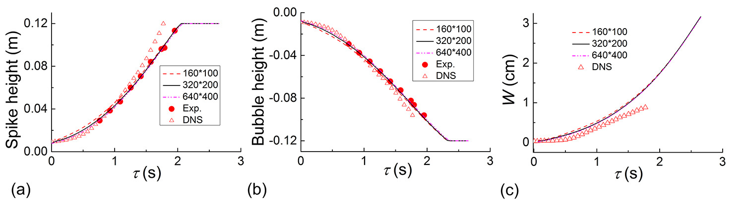
2D simulations of buoyancy-driven flow are performed with three grid sizes, $160\times 100$, $320\times 200$, and $640\times 400$, and the results are presented in Figure 3 comparing with the experimental data (Smeeton & Youngs, 1987) and numerical results (Andrews et al., 2014). All the numerical results of the three resolutions agree very well with the experiments and simulations. Very good grid convergence is obtained since the difference between the resolutions $320\times 200$ and $640\times 400$ is negligible. Therefore, grid size $320\times 200$ is employed in the following simulations.

We first performed the eigenspace perturbation in Reynolds stress. The uncertainty bounds for spike and bubble height and the mixing width are presented in Figure 4. The uncertainty intervals for all the quantities are negligible, which shows that the term $P$ in the turbulent kinetic energy transport equation should be very small for this buoyancy-driven flow. Therefore, the alignment or misalignment between the eigenvector of Reynolds stress and mean rate of strain is insufficient to affect the variable-density flow.

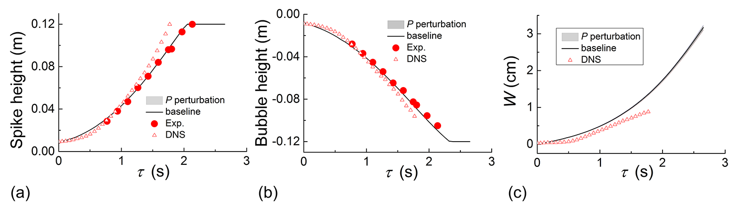
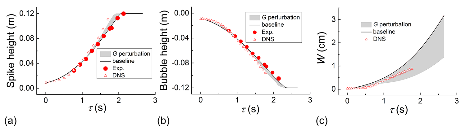
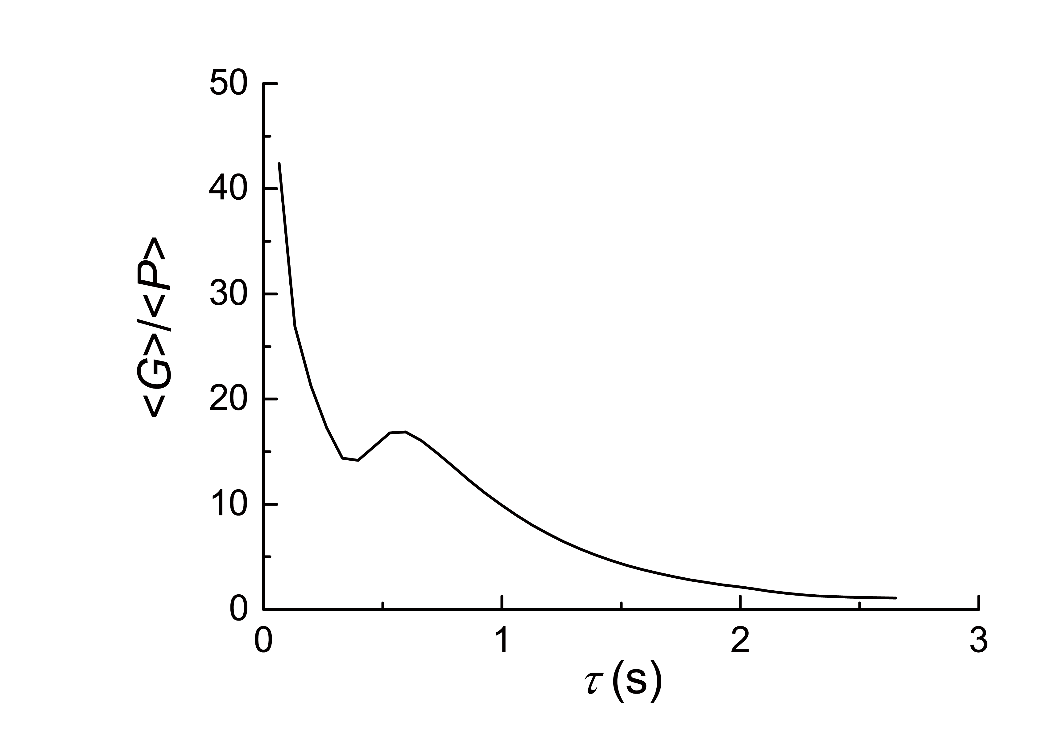
In the 2D set up, the angle between the vectors $\mathbb{a}$ and $\mathbb{p}_{g}$ could be varying from 0 to $\pi$. Since the flow is driven by buoyancy, the turbulent mass-flux velocity is most likely to obey the density gradient, or pressure gradient, and the angle between $\mathbb{a}$ and $\mathbb{p}_{g}$ varying from 0 to $\pi/2$ is more reasonable. Therefore, the term $G=\mathbb{a}\cdot\mathbb{p}_{g}$ has the range $0\leq G\leq\mid\mathbb{a}\mid\mid\mathbb{p}_{g}\mid$, where $\mid\mid$ is the magnitude of the vector. Consequently, the two extreme cases of $G$ for buoyancy-driven flow are simulated, and the uncertainty estimation is shown in Figure 5 in comparison to experimental data and DNS results. The uncertainty interval is significantly increased for $G$ perturbation compared with that of $P$ eigenspace perturbation, and enables us to account for the discrepancy between experimental observations and DNS results. The ratio between the volume integral of $G$ and $P$, $\langle G\rangle/\langle P\rangle$ where $\langle\psi\rangle=\int_{V}\psi dV$ , is shown in Figure 6. It is obvious that the term $G$ is much larger than $P$, which explains the negligible uncertainty estimation of eigenspace perturbation in Reynolds stress shown in Figure 4.

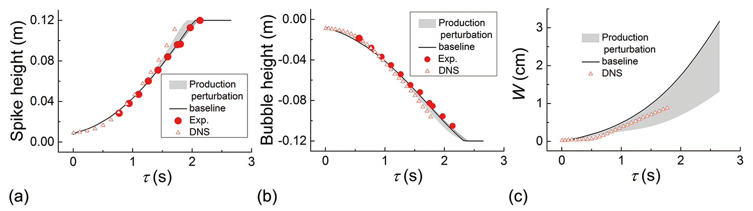
Finally, the BHR model uncertainty is quantified by perturbing the two terms $G$ and $P$ together in the production. The uncertainty interval, shown in Figure 7, is captured by the 10 extreme states.

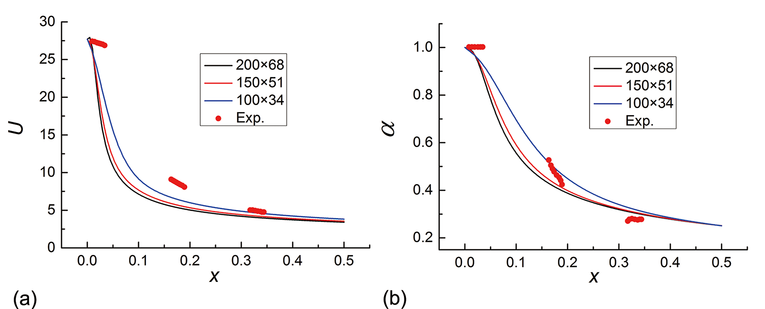
In the above simulations, the flows are driven by buoyancy due to the variable density. Here, we consider the effect of density gradients on the transport of fluid and the evolution of the turbulent characteristics of the turbulent jet mixing flow. The turbulent jet flow has been studied experimentally by Charonko & Prestridge (2017) using particle image velocimetry (PIV) and planar laser-induced fluorescence (PLIF) measurements. The jet flow is supplied using a $d_{0}=11$ mm inner-diameter tube vertically oriented in an open-circuit wind tunnel with a $0.53\times 0.53$ m cross section. The acetone and gas mixture in the jet has density $\rho_{1}=1.1$ g/cm³, while the density of ambient air is $\rho_{2}=0.92$ g/cm³, which results in Atwood number $At=0.09$. The inlet velocity of the jet is $27.7$ m/s, while the coflowing ambient air has velocity $1.4$ m/s. To simulate the flow, a jet with diameter $d_{0}=11$ mm in a circular channel with radius $r=25$ cm is chosen for the computational domain, the inlet turbulent kinatic energy of the jet $k=20.0$ m²/s² is selected. The calculated velocity and the mass fraction with different mesh sizes are compared with experimental data in Figure 8. The numerical results show reasonable agreement with experimental data, and the mesh size $150\times 51$ is chosen for the following simulations.

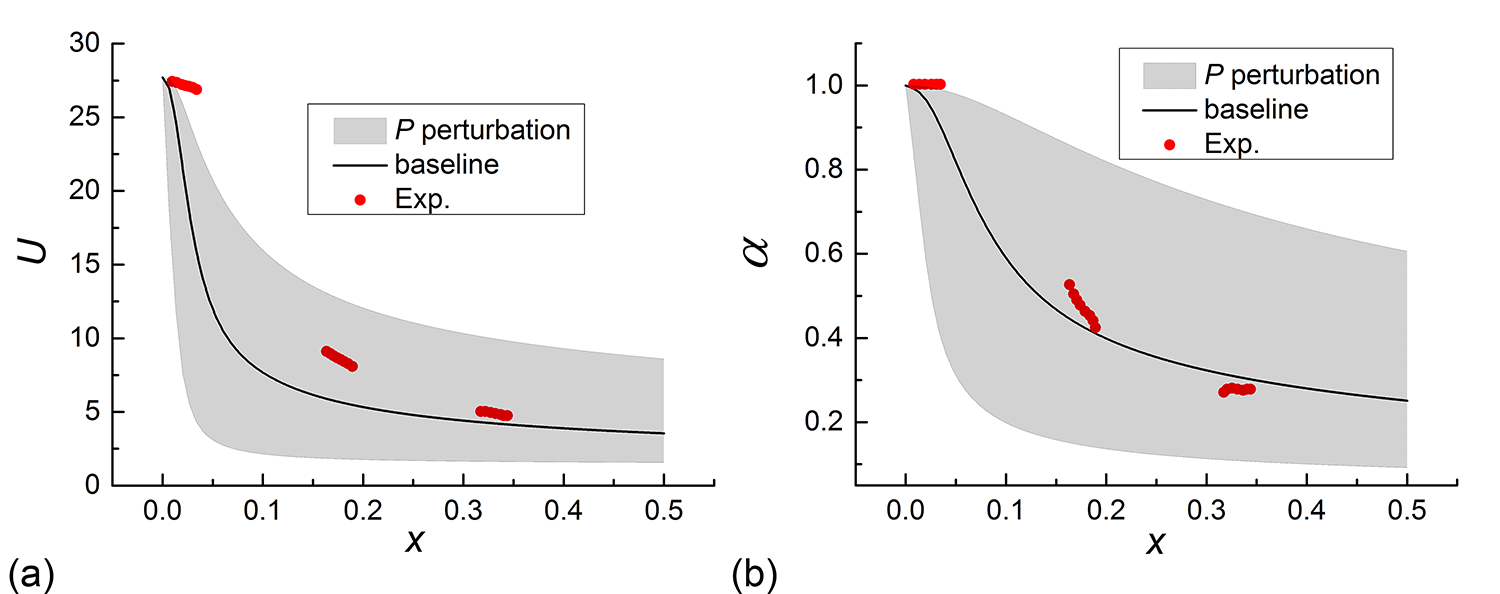
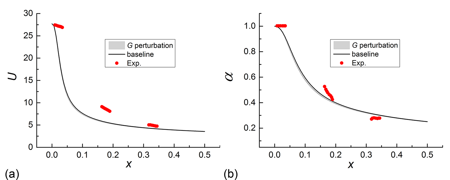
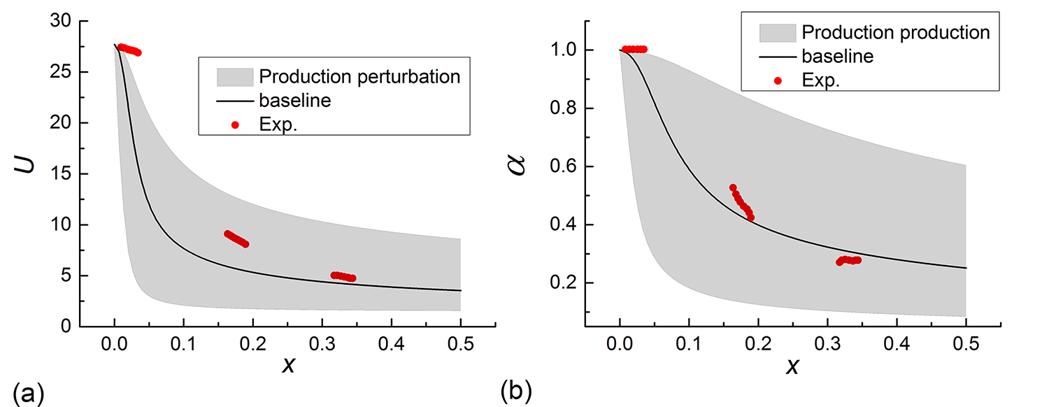
Unlike the TR case, the values of volume-averaged $P$ is about 24 times that of $G$ for the turbulent jet mixing flow, which means that $P$ is dominant. The uncertainty interval of eigenspace perturbation in $P$ is shown in Figure 9. The eigenspace perturbation bounds are able to account for the discrepancy between model predictions and experimental data except near the jet inlet, as expected since $P$ is dominant. In contrast, the uncertainty estimation of the $G$ term perturbation is negligible, as shown in Figure 10. The structural uncertainty quantified by maximizing and minimizing the production in the BHR model is shown in Figure 11 by simulating the 10 extreme cases. Due to the combination of the eigenspace perturbation in $P$ and the perturbation in $G$, the perturbation of the production quantifies the structural uncertainty.

References

- Andrews et al. (2014) Andrews, M. J., Youngs, D. L., Livescu, D. & Wei, T. 2014 Computational studies of two-dimensional Rayleigh-Taylor driven mixing for a tilted-rig. J. Fluids Eng. 136, 091212.
- Banerjee et al. (2010) Banerjee, A., Gore, R. A. & Andrews, M. J. 2010 Development and validation of a turbulent-mix model for variable-density and compressible flows. Phys. Rev. E 82, 046309.
- Banerjee et al. (2010) Banerjee, A., Kraft, W. N. & Andrews, M. J. 2010 Detailed measurements of a statistically steady Rayleigh–Taylor mixing layer from small to high Atwood numbers. J. Fluid Mech. 659, 127-190.
- Besnard et al. (1992) Besnard, D., Harlow, F. H., Rauenzahn, R. M. & Zemach,C. 1992 Turbulence transport equations for variable density turbulence and their relationship to two-field models. LANL Report LA-12303-MS.
- Boyd (2018) Boyd, J. P. 2018 Dynamics of the Equatorial Ocean. Burlin:Springer.
- Charonko & Prestridge (2017) Charonko, J. J. & Prestridge, K. 2017 Variable-density mixing in turbulent jets with coflow. J. Fluid Mech. 825, 887-921.
- Emory et al. (2013) Emory, M., Larsson, J. & Iaccarino, G. 2013 Modeling of structural uncertainties in Reynolds-averaged Navier-Stokes closures. Phys. Fluids 25, 110822.
- Gorlé & Iaccarino (2013) Gorlé, C. & Iaccarino, G. 2013 A framework for epistemic uncertainty quantification of turbulent scalar flux models for Reynolds-averaged Navier-Stokes simulations. Phys. Fluids 25, 055105.
- Gorlé et al. (2015) Gorlé, C., Garcia-Sanchez C. & Iaccarino, G. 2013 Quantifying inflow and RANS turbulence model form uncertainties for wind engineering flows. J. Wind Eng. Ind. Aerodyn. 144, 202-212.
- Iaccarino et al. (2017) Iaccarino, G., Mishra, A. A. & Ghili, S. 2017 Eigenspace perturbations for uncertainty estimation of single-point turbulence closures. Phys. Rev. Fluids 2, 024605.
- Kokkinakis et al. (2019) Kokkinakis, I. W., Drikakis, D. & Youngs, D. L. 2019 Modeling of Rayleigh-Taylor mixing using single-fluid models. Phys. Rev. E 99, 013104.
- Lindl et al. (1992) Lindl, J. D., Mccrory, R. L. & Campbell, E. M. 1992 Progress toward ignition and burn propagation in inertial confinement fusion. Phys. Today 45, 32-40.
- Mishra & Iaccarino (2016) Mishra, A. A. & Iaccarino, G. 2016 RANS predictions for high-speed flows using enveloping models. Annual Research Briefs, Center for Turbulence Research, Stanford University, pp. 289-301.
- Mishra & Iaccarino (2017) Mishra, A. A. & Iaccarino, G. 2017 Uncertainty estimation for Reynolds averaged Navier-Stokes predictions of high-speed aircraft nozzle jets. AIAA J. 55, 11.
- Schwarzkopf et al. (2016) Schwarzkopf, J. D., Livescu, D., Baltzer, J. R., Gore, R. A. & Ristorcelli, J. R. 2016 A Two-length scale turbulence model for single-phase multi-fluid mixing. Flow, Turbul. Combust. 96, 1-43.
- Schwarzkopf et al. (2011) Schwarzkopf, J. D., Livescu, D., Gore, R. A., Rauenzahn, R. M. & Ristorcelli, J. R. 2016 Application of a second-moment closure model to mixing processes involving multicomponent miscible fluids. J. Turbul. 49, 1-35.
- Smeeton & Youngs (1987) Smeeton, V. S. & Youngs, D. L. 1987 Experimental investigation of turbulent mixing by Rayleigh-Taylor instability III. AWE Report O35/87.
- Thompson et al. (2019) Thompson, R. L., Mishra, A. A., Iaccarino, G., Edeling, W. & Sampaio L. 2019 Eigenvector perturbation methodology for uncertainty quantification of turbulence models. Phys. Rev. Fluids 4, 044603.
- Youngs (1989) Youngs, D. L. 1989 Modeling turbulent mixing by Rayleigh-Taylor instability. Physica D 3, 270–287.
- Zingale et al. (2009) Zingale, M., Almgren, A. S., Bell, J. B., Nonak, A. & Woosley, S. E. 2009 Low Mach number modeling of type IA supernovae. IV. White dwarf convection. Astrophys. J. 704, 196–210.