Quantifying Uncertainty for Machine Learning Based Diagnostic

Particle accelerators serve a wide variety of applications ranging from chemistry, physics to biology experiments. Those experiments require increased accuracy of diagnostics tools to measure the electron beam properties during its acceleration, transport and delivery to users. Current state-of-the-art diagnostics (Marx et al. 2018a) have limited applicability as the complexity of the experiments grows. Virtual diagnostic (VD) tools provide a shot-to-shot non-invasive measurement of the beam in cases where the diagnostic has limited resolution or unavailable. VDs have the potential to be useful also in experiments design, setup and optimization while saving valuable operation time. They could also aid in interpreting experimental results, especially in cases in which current diagnostics cannot provide necessary information. In this extended abstract, we apply deep learning tools to provide confidence interval of the virtual diagnostic prediction using experimental data from the Linac Coherent Light Source (LCLS) at SLAC.

Current VD provides predictive models based on training a neural network mapping between non-invasive diagnostic input to invasive output measurement (Emma et al. 2018; Hanuka et al. 2021). This type of mapping is known as supervised regression. Previous work has demonstrated VD to predict the electron beam current profile and Longitudinal Phase Space (LPS) distribution (Marx et al. 2018b) along the accelerator using either scalar controls (Emma et al. 2018) or spectral information (Hanuka et al. 2021) as the non-invasive input to the VD. However, an essential component in deploying the virtual diagnostic tool is to quantify the confidence in the prediction, i.e. estimate an interval presenting the uncertainty in prediction. This becomes critical in systems such as particle accelerators, where safety is of highest concern. In addition, users must have a reliable presentation of uncertainty given a set of inputs in order to make informed decisions.

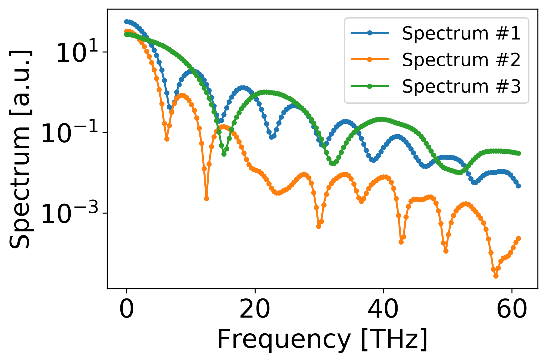
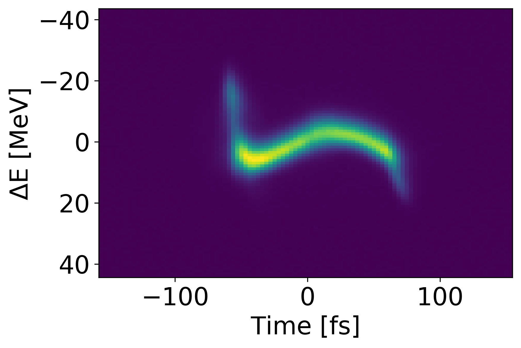
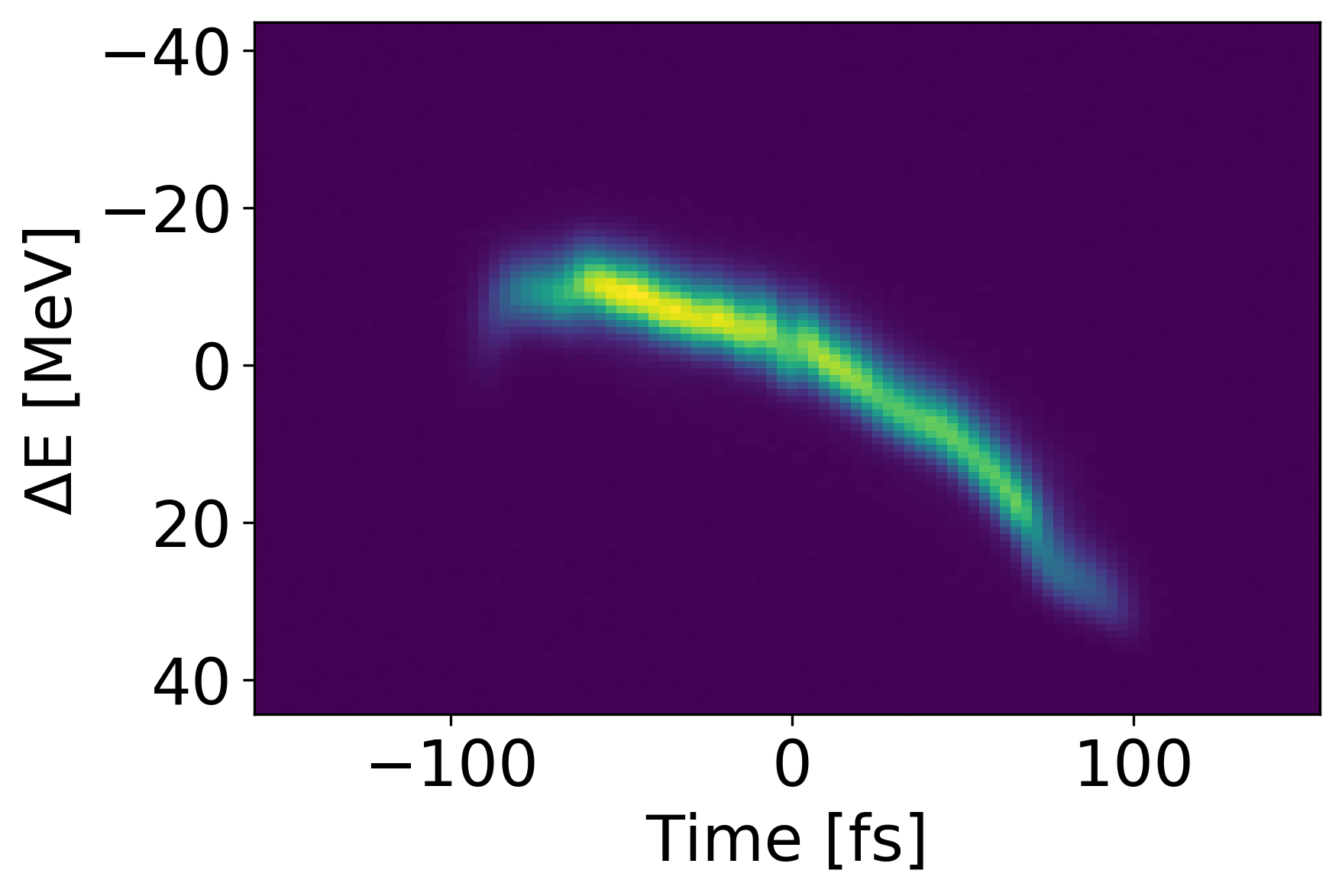
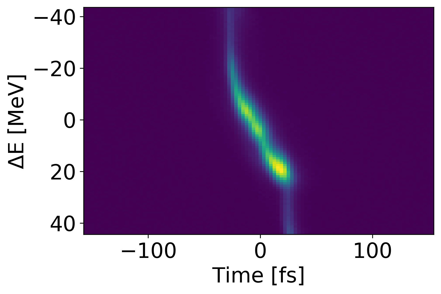
High brightness beam linacs typically operate in single-pass, multi-stage configurations where a high-density electron beam formed in the RF gun is accelerated and manipulated prior to delivery to users in an experimental station. An example of such a facility is the LCLS XFEL at SLAC where the electron beam traverses through an undulator, and emits coherent X-ray pulses. Typically, longitudinal phase space (LPS) is destructively measured by X-band transverse deflecting cavity (XTCAV) (Marx et al. 2018a). In this abstract we used a longitudinal phase space (LPS) data set measured at the XTCAV, as the outputs, and the corresponding spectral information, as can be collected by the IR spectrometer, as an input.

Deep ensembles are ensembles of neural networks, each initialised differently and optimised to convergence independently of the others. Ref. (Lakshminarayanan, Pritzel, and Blundell 2017) has shown empirically that explicit ensembling can result in improved uncertainty estimates when they used large neural networks with non-convex loss surfaces.

The predicted current profile for a test shot $\vec{I}_{{\rm predicted}}=M^{-1}\sum_{m=1}^{M}\vec{i}_{{\rm predicted},m}$ is the mean prediction of $M$ neural network predictions $\vec{i}_{{\rm predicted},m}$. The uncertainty is manifested as the standard deviation of the neural network predictions $\vec{\sigma}=\sqrt{M^{-1}\sum_{m=1}^{M}(\vec{i}_{{\rm predicted},m}-\vec{I}_{\rm predicted})^{2}}$.

The neural network (NN) architecture we used is a fully connected feed-forward NN composed of three hidden layers (200, 100, 50) with rectified linear unit activation function. For training we used batch size of 32, 500 epochs and Adam optimizer with fixed learning rate of 0.001 in our experiments (Hanuka et al. 2021). Training the NNs with a Gaussian likelihood, i.e. to minimize the standard Mean Squared Error (MSE) loss function on a training set, yields symmetric uncertainty intervals. For all the examples presented we use the open source Keras and TensorFlow libraries to build and train the NN module (Chollet et al. 2015; Abadi et al. 2015).

To evaluate the mean prediction of our VD, we use the standard mean squared error metrics (${\rm MSE}={T^{-1}\sum_{t=1}^{T}{(I_{{\rm measured},t}-I_{{\rm predicted},t})}^{2}}$). To evaluate the uncertainty intervals provided by the predictive standard deviation, we use a custom accuracy metric:

where ${\rm\alpha}_{t}=1$ if $I_{\rm lower}{,t}<I_{{\rm measured}{,t}}<I_{{\rm upper}{,t}}$ and 0 otherwise. We used bounds of $I_{{\rm predicted}{,t}}\pm 2\sigma_{t}$ where $\sigma_{t}$ is predictive standard deviation at time $t$.

The average MSE of the VD on the test set is 6.714e-04 with an accuracy of 0.538 using $\pm 2\sigma$. Figure 2 shows an example of a poor test shot with a few tools to analyze the VD performance. We present a comparison between the VD prediction and ground truth on the left, and the ground truth with red indicating where the prediction is accurate.

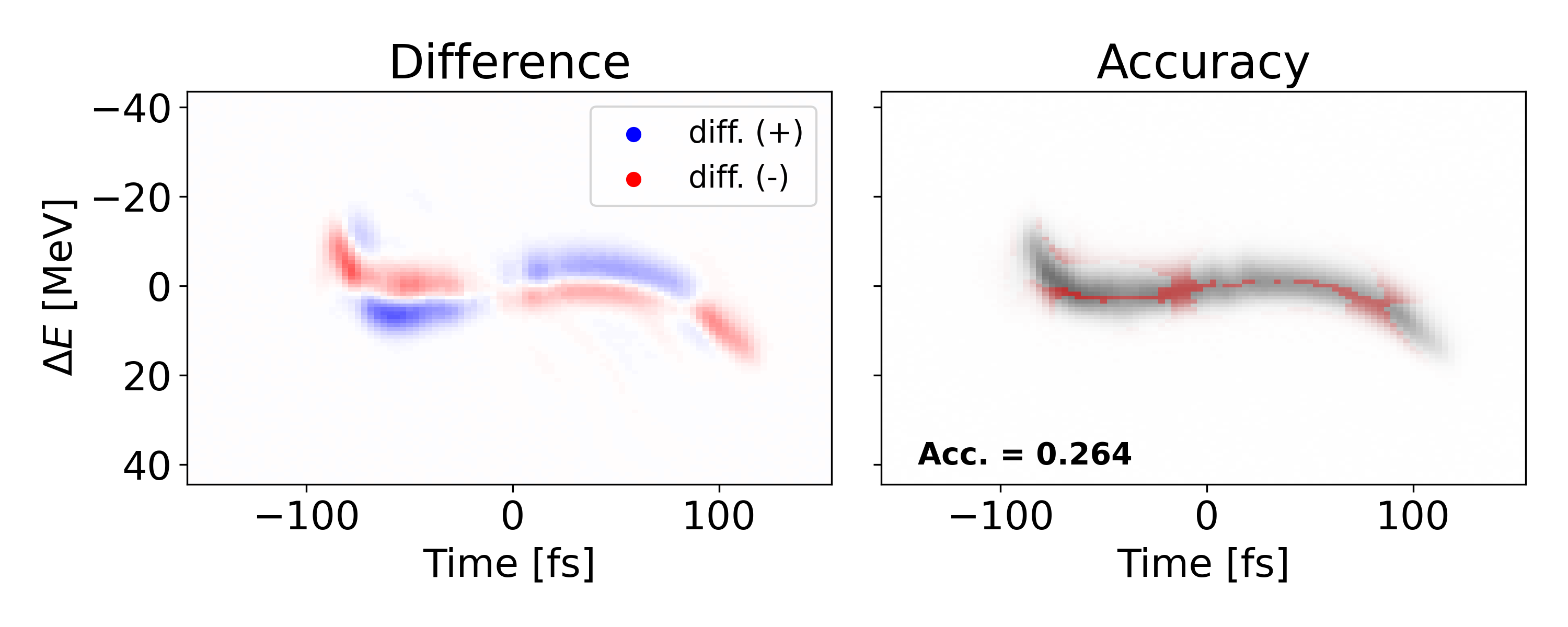
In the shown test shot we observe a large MSE of 1.096e-3 and a low accuracy of 0.208. The large MSE becomes obvious when we look at the second panel depicting the error. In the case of this shot, the shape of the prediction is completely off. Looking at the right most panel, we see the prediction is the most uncertain near the tails of the signal and confident near the center.

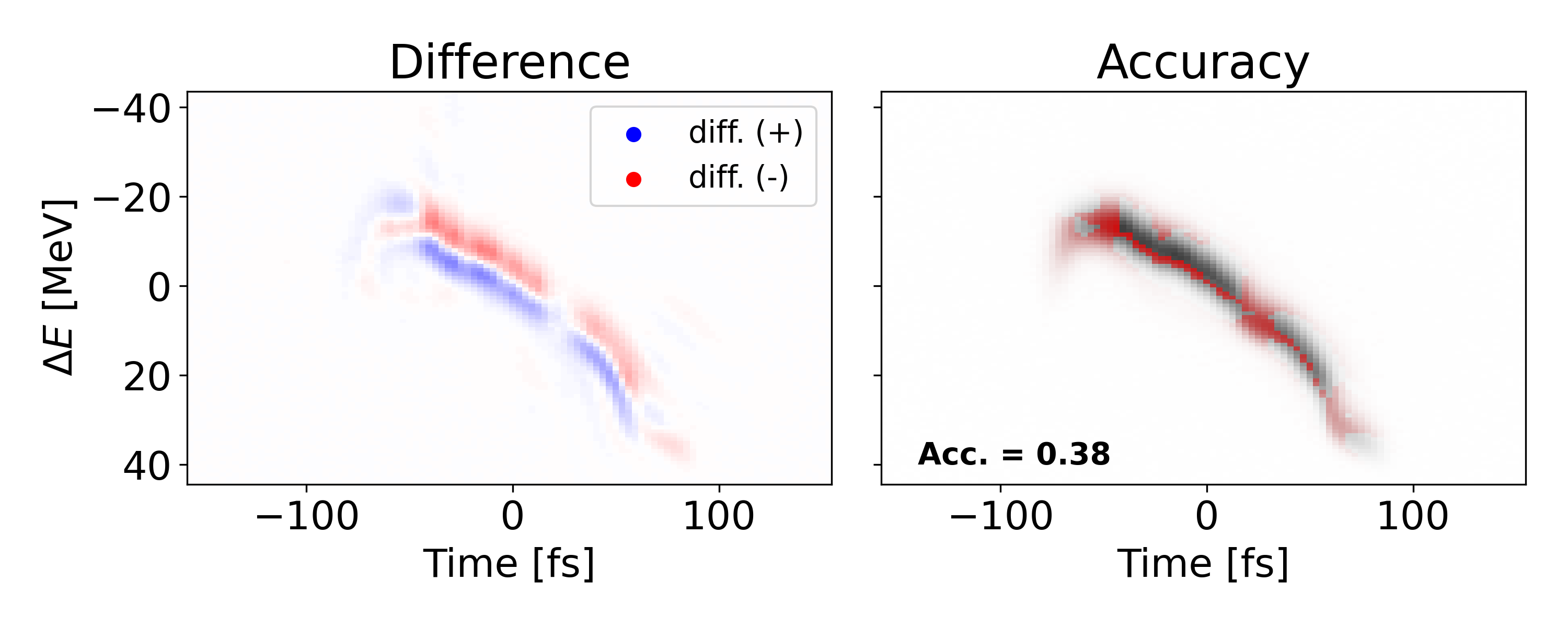
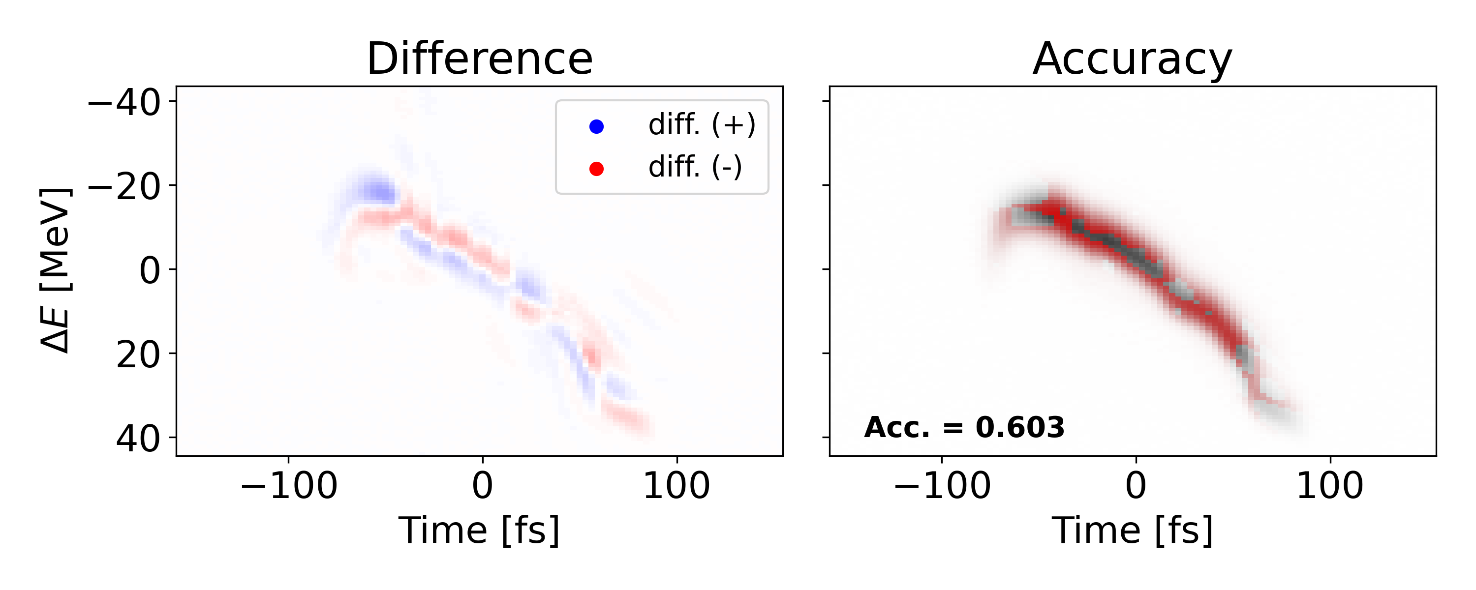
Another poor shot is shown above with an MSE of 2.737e-4 and accuracy of 0.383. However, this lower performance is due to translational error, not shape error as seen in the previous example. Since we mostly care about the shape of the signal, we can translate the prediction to match the ”center of mass” for the measured value. Doing so yields an MSE of 8.396e-5 and and accuracy of 0.661 which indicates an improvement of 85.0$\%$ and 41.8$\%$ respectively. Both types of error could potentially be reduced if spatial connectivity was leveraged in a more sophisticated network architecture.

In this abstract we have presented methods, metrics, and tools to present uncertainty quantification for standalone LPS images. Although looking at individual shots allows us pinpoint data set features and analyze problems with our VD, it does not give much insight into how the VD performs on the data set as a whole. In future research, we will present tools to visualize uncertainty over an entire test set and allow users to make crucial decisions regarding rejection thresholds and machine operations.

This work was supported by the Department of Energy, Laboratory Directed Research and Development program at SLAC National Accelerator Laboratory, under contract DE-AC02-76SF00515.

References

- Abadi et al. (2015) Abadi, M.; Agarwal, A.; Barham, P.; Brevdo, E.; Chen, Z.; Citro, C.; Corrado, G. S.; Davis, A.; Dean, J.; Devin, M.; Ghemawat, S.; Goodfellow, I.; Harp, A.; Irving, G.; Isard, M.; Jia, Y.; Jozefowicz, R.; Kaiser, L.; Kudlur, M.; Levenberg, J.; Mané, D.; Monga, R.; Moore, S.; Murray, D.; Olah, C.; Schuster, M.; Shlens, J.; Steiner, B.; Sutskever, I.; Talwar, K.; Tucker, P.; Vanhoucke, V.; Vasudevan, V.; Viégas, F.; Vinyals, O.; Warden, P.; Wattenberg, M.; Wicke, M.; Yu, Y.; and Zheng, X. 2015. TensorFlow: Large-Scale Machine Learning on Heterogeneous Systems. URL http://tensorflow.org/. Software available from tensorflow.org.
- Chollet et al. (2015) Chollet, F.; et al. 2015. Keras. https://keras.io.
- Emma et al. (2018) Emma, C.; Edelen, A.; Hogan, M. J.; O’Shea, B.; White, G.; and Yakimenko, V. 2018. Machine learning-based longitudinal phase space prediction of particle accelerators. Phys. Rev. Accel. Beams 21: 112802. doi:10.1103/PhysRevAccelBeams.21.112802. URL https://link.aps.org/doi/10.1103/PhysRevAccelBeams.21.112802.
- Hanuka et al. (2021) Hanuka, A.; Emma, C.; Maxwell, T.; Fisher, A.; Jacobson, B.; Hogan, M. J.; and Huang, Z. 2021. Accurate and confident prediction of electron beam longitudinal properties using spectral virtual diagnostics. Nature Scientific Reports 11: 2945. URL ”https://doi.org/10.1038/s41598-021-82473-0”.
- Lakshminarayanan, Pritzel, and Blundell (2017) Lakshminarayanan, B.; Pritzel, A.; and Blundell, C. 2017. Simple and scalable predictive uncertainty estimation using deep ensembles. In Advances in neural information processing systems, 6402–6413. San Diego, CA: NeurIPS. URL https://papers.nips.cc/paper/2017/hash/9ef2ed4b7fd2c810847ffa5fa85bce38-Abstract.html.
- Marx et al. (2018a) Marx, D.; Assmann, R.; Craievich, P.; Dorda, U.; Grudiev, A.; and Marchetti, B. 2018a. Longitudinal phase space reconstruction simulation studies using a novel X-band transverse deflecting structure at the SINBAD facility at DESY. Nuclear Instruments and Methods in Physics Research Section A: Accelerators, Spectrometers, Detectors and Associated Equipment 909: 374–378. ISSN 0168-9002. doi:https://doi.org/10.1016/j.nima.2018.02.037. URL http://www.sciencedirect.com/science/article/pii/S0168900218301918. 3rd European Advanced Accelerator Concepts workshop (EAAC2017).
- Marx et al. (2018b) Marx, D.; Assmann, R.; Craievich, P.; Dorda, U.; Grudiev, A.; and Marchetti, B. 2018b. Longitudinal phase space reconstruction simulation studies using a novel X-band transverse deflecting structure at the SINBAD facility at DESY. Nuclear Instruments and Methods in Physics Research Section A: Accelerators, Spectrometers, Detectors and Associated Equipment 909: 374 – 378. ISSN 0168-9002. doi:https://doi.org/10.1016/j.nima.2018.02.037. URL http://www.sciencedirect.com/science/article/pii/S0168900218301918. 3rd European Advanced Accelerator Concepts workshop (EAAC2017).