Quantile Reinforcement Learning

Markov Decision Processes (MDPs) offer a powerful formalism to model and solve sequential decision-making problems (Puterman, 1994). A finite horizon MDP is formally defined as a tuple $\mathcal{M}_{T}=(S,A,\mathbf{P},\mathbf{R},s_{0})$ where:

• •

  $T$ is a finite horizon,

• •

  $S$ is a finite set of states,

• •

  $A$ is a finite set of actions,

• •

  $\mathbf{P}:S\times A\times S\rightarrow\mathbb{R}$ is a transition function with $\mathcal{P}(s,a,s^{\prime})$ being the probability of reaching state $s^{\prime}$ when action $a$ is performed in state $s$,

• •

  $\mathbf{R}:S\times A\rightarrow\mathbb{R}$ is a bounded reward function and

• •

  $s_{0}\in S$ is an initial state.

In this model, starting from initial state $s_{0}$, an agent chooses at every time step $t$ an action $a_{t}$ to perform in her current state $s_{t}$, which she can observe. This action results in a new state $s_{t+1}\in S$ according to probability distribution $\mathbf{P}(s_{t},a_{t},.)$, and a reward signal $\mathbf{R}(s_{t},a_{t})$, which penalizes or reinforces the choice of this action.

We will call $t$-history $h_{t}$ a succession of $t$ state-action pairs starting from state $s_{0}$ (e.g., $h_{t}=(s_{0},a_{1},s_{1},\ldots,s_{t-1},a_{t-1},s_{t})$). The action choices of the agent is guided by a policy. More formally, a policy $\pi$ at an horizon $T$ is a sequence of $T$ decision rules $(\delta_{T},\ldots,\delta_{1})$. Decision rules prescribe which action the agent should perform at a given time step. They can be Markovian if they only depend on the current state. Besides, a decision rule is either deterministic if it always selects the same action in a given situation or randomized if it prescribes a probability distribution over possible actions. Consequently, a policy can be Markovian, deterministic or randomized according to the type of its decision rules. Lastly, a policy is stationary if it applies the same decision rule at every time step, i.e., $\pi=(\delta,\delta,\ldots)$.

Policies can be compared with respect to different decision criteria. The usual criterion is the expected (discounted) sum of rewards, for which an optimal deterministic Markovian policy is known to exist for any horizon $T$. This criterion is defined as follows. First, the value of a history $h_{t}=(s_{0},a_{1},s_{1},\ldots,s_{t-1},a_{t},s_{t})$ is described as the (possibly discounted) sum of rewards obtained along it, i.e.,

where $\gamma\in[0,1]$ is a discount factor. Then, the value of a policy $\pi=(\delta_{T},\ldots,\delta_{1})$ in a state $s$ is set to be the expected value of the histories that can be generated by $\pi$ from $s$. This value, given by the value function $v^{\pi}_{T}:S\to\mathbb{R}$ can be computed iteratively as follows:

The value $v^{\pi}_{t}(s)$ is the expectation of cumulated rewards obtained by the agent if she performs action $\delta_{t}(s)$ in state $s$ at time-step $t$ and continues to follow policy $\pi$ thereafter. The higher the values of $v^{\pi}_{t}(s)$ are, the better. Therefore, value functions induce a preference relation $\succsim_{\pi}$ over policies in the following way:

A solution to an MDP is a policy, called optimal policy, that ranks the highest with respect to $\succsim_{\pi}$. Such a policy can be found by solving the following equations, which yields the value function of an optimal policy:

In the reinforcement learning (RL) setting, the assumption of the knowledge of the environment is relaxed: both dynamics through the transition function and preferences via the reward function are not known anymore. While interacting with its environment, an RL agent tries to learn a good policy by trial and error.

To make finite horizon MDPs learnable, we assume the decision process is repeated infinitely many times. That is, when horizon $T$ is reached, we assume that the agent automatically returns to the initial state and the problem starts over.

A simple algorithm to solve such an RL problem is the Q-learning algorithm (see Algorithm 1), which estimates the Q-function:

And obviously, we have: $V_{t}(s)=\displaystyle\max_{a\in A}Q_{t}(s,a)$.

In Algorithm 1, Line 1 generally depends on the $Q_{t-1}(s,\cdot)$ and possibly on iteration $n$. A simple strategy to perform this choice is called $\varepsilon$-greedy where the best action dictated by $Q_{t-1}(s,\cdot)$ is chosen with probability $1-\varepsilon$ (with $\varepsilon$ a small positive value) or a random action is chosen otherwise. A schedule can be defined so that parameter $\varepsilon$ tends to zero as $n$ tends to infinity. Besides, $\alpha_{n}(s,a)\in(0,1)$ on Line 1 is a learning rate. In the general case, it depends on iteration $n$, state $s$ and action $a$, although in practice it is often chosen as a constant.

The standard decision criteria used in MDPs, which are based on expectation, may not be reasonable in some situations. Firstly, unfortunately, in many cases, the reward function $\mathbf{R}$ is not known. In those cases, one can try to recover the reward function from a human expert (Ng and Russell, 2000; Regan and Boutilier, 2009; Weng and Zanuttini, 2013). However, even for an expert user, the elicitation of the reward function can reveal burdensome. In inverse reinforcement learning (Ng and Russell, 2000), the expert is assumed to know an optimal policy, which is rarely true in practice. In interactive settings (Regan and Boutilier, 2009; Weng and Zanuttini, 2013), this elicitation process can be cognitively very complex as it requires to balance several criteria in a complex manner and as it can imply a large number of parameters. In this paper, we address this problem by only assuming that a strict weak ordering over histories is known.

Secondly, for numerous applications, the expectation of cumulated reward, as used in Equation 1, may not be the most appropriate criterion (even when a numeric reward function is defined). For instance, in case of high variance or when a policy is known to be only applied a few times, the solution given by this criterion may not be satisfying for risk-averse agent. Moreover, in some domains (e.g., web industry or more generally service industry), decisions about performance are often based on the minimal quality of $99\%$ of the possible outcomes. Therefore, in this article we aim at using a quantile (defined in Section 3.5) as a decision criterion to solve an MDP.

In this paper, we work with episodic MDPs with end states. Such an MDP is formally defined as a tuple $\mathcal{M}_{T}=(S,A,G,\mathbf{P},s_{0})$ where $S$, $A$, $\mathbf{P}$, $s_{0}$ are defined as previously, $G\subseteq S$ is a finite set of end states and $T$ is a finite maximal horizon (i.e., an end state is attained after at most $T$ time steps.). We call episode a history starting from $s_{0}$ and ending in a final state of $G$.

We assume that a preference relation is defined over end states: We write $g^{\prime}\prec g$ if end state $g$ is preferred to end state $g^{\prime}$. Without loss of generality, we assume that $G=\{g_{1},\ldots,g_{n}\}$ and end states are ordered with increasing preference, i.e., $g_{1}\prec g_{2}\prec\ldots\prec g_{n}$. The weak relation of $\prec$ is denoted $\preceq$.

Note that a finite horizon MDP can be reformulated as an MDP with end states by state augmentation. Although the resulting MDP may have a large-sized state space, the two models are formally equivalent. We focus on episodic MDPs with end states to simplify the presentation of our approach.

We define quantiles of distributions over end states of $G$, which are ordered by $\preceq$. Let $\tau\in[0,1]$ be a fixed parameter. Intuitively, the $\tau$-quantile of a distribution of end states, is the value $q\in G$ such that the probability of getting an end state equal or lower than $q$ is $\tau$ and that of getting an end state equal or greater than $q$ is $1-\tau$. The $0.5$-quantile, also known as median, can be seen as the ordinal counterpart of the mean. The $0$-quantile (resp. $1$-quantile) is the minimum (resp. maximum) of a distribution. More generally, quantiles, which have been axiomatically characterized by Rostek (2010), define decision criteria that have the nice property of not requiring numeric valuations, but only an order.

The formal definition of quantiles can be stated as follows. Let $p^{\pi}$ denote the probability distribution over end states induced by a policy $\pi$ from initial state $s_{0}$, the cumulative distribution induced by $p^{\pi}$ is then defined as $F^{\pi}$ where $F^{\pi}(g)=\sum_{g^{\prime}\preceq g}p^{\pi}(g^{\prime})$ is the probability of getting an end state not preferred to $g$ when applying policy $\pi$. Similarly, the decumulative distribution induced by $p^{\pi}$ is defined as $G^{\pi}(g)=\sum_{g\preceq g^{\prime}}p^{\pi}(g^{\prime})$ is the probability of getting an end state not lower than $g$.

These two notions of cumulative and decumulative enable us to define two kinds of criteria. First, given a policy $\pi$, we define the lower $\tau$-quantile for $\tau\in(0,1]$ as:

where the $\min$ operator is with respect to $\preceq$.

Then, given a policy $\pi$, we define the upper $\tau$-quantile for $\tau\in[0,1)$ as:

where the $\max$ operator is with respect to $\preceq$.

If $\tau=0$ or $\tau=1$ only one of $\underline{q}_{\tau}^{\pi}$ or $\overline{q}_{\tau}^{\pi}$ is defined and we define the $\tau$-quantile $q_{\tau}^{\pi}$ as that value. When both are defined, by construction, we have $\underline{q}_{\tau}^{\pi}\preceq\overline{q}_{\tau}^{\pi}$. If those two values are equal, $q_{\tau}^{\pi}$ is defined as equal to them. For instance, this is always the case in continuous settings for continuous distributions. However, in our discrete setting, it could happen that those values differ, as shown by Example 1.

When the lower and the upper quantiles differ, one may define the quantile as a function of the lower and upper quantiles (Weng, 2012). For simplicity, in this paper, we focus on optimizing directly the lower and the upper quantiles.

The quantile criterion is difficult to optimize, even when a numerical reward function is given and the quality of an episode is defined as the cumulative of rewards received along the episode. This difficulty comes notably from two related sources:

• •

  The quantile criterion is non-linear: for instance, the $\tau$-quantile $q_{\tau}^{\tilde{\pi}}$ of the mixed policy $\tilde{\pi}$ that generates an episode using policy $\pi$ with probability $p$ and $\pi^{\prime}$ with probability $1-p$ is not equal to $pq_{\tau}^{\pi}+(1-p)q_{\tau}^{\pi^{\prime}}$.

• •

  The quantile criterion is non-dynamically consistent: A sub-policy at time step $t$ of an optimal policy for horizon $T$ may not be optimal for horizon $T-t$.

In decision theory (McClennen, 1990), three approaches have been considered for such kinds of decision criteria:

1. 1.

   Consequentialist approach: at each time step $t$, follow an optimal policy for the problem with horizon $T-t$ and initial state $s_{t}$ even if the resulting policy is not optimal at horizon $T$;

2. 2.

   Resolute choice approach: at time step $t=0$, apply an optimal policy for the problem with horizon $T$ and initial state $s_{0}$ and do not deviate from it;

3. 3.

   Sophisticated resolute choice approach (Jaffray, 1998; Fargier et al., 2011): apply a policy $\pi$ (chosen at the beginning) that trades off between how much $\pi$ is optimal for all horizons $T,T-1,\ldots,1$.

With non-dynamically consistent preferences, it is debatable to adopt a consequentialist approach, as the sequence of decisions may lead to dominated results. In this paper, we adopt a resolute choice point of view. We leave the third approach for future work.

In this paper, we aim at learning a policy that is optimal for the quantile criterion from a fixed initial state. We assume that the underlying MDP is an episodic MDP with end states. Let $\tau\in(0,1)$ be a fixed parameter. Formally, the problem of determining a policy optimal for the lower/upper $\tau$-quantile can be stated as follows:

We focus on learning a policy that is deterministic and Markovian.

The optimal lower/upper quantiles satisfy the following lemmas:

Then, if the optimal lower quantile ($\underline{q}^{*}_{\tau}$) or upper quantile ($\overline{q}^{*}_{\tau}$) were known, the problem would be relatively easy to solve. By Lemma 1, an optimal policy for the lower quantile could be obtained as follows:

where $\underline{q}^{-}_{\tau}=g_{1}$ if $\underline{q}^{*}_{\tau}=g_{1}$ and $\underline{q}^{-}_{\tau}=g_{i}$ if $\underline{q}^{*}_{\tau}=g_{i+1}$. The reason one needs to use $\underline{q}^{-}_{\tau}$ instead of the optimal lower quantile is that otherwise it may happen that the cumulative distribution of a non-optimal policy $\pi$ is smaller than or equal to that of an optimal policy at the lower quantile $\underline{q}^{*}_{\tau}$ (but greater below $\underline{q}^{*}_{\tau}$ as $\pi$ is not optimal). In that case, the lower quantile of $\pi$ might not be $\underline{q}^{*}_{\tau}$. Such a thing cannot happen for the upper quantile. In that sense, determining an optimal policy for the upper quantile is easier. By Lemma 1, it is simply given by:

In practice, if the lower/upper quantiles were known, those policies could be computed by solving a standard MDP with the following reward functions:

for the lower quantile with $\theta=k$ if $\underline{q}^{-}_{\tau}=g_{k}$ and

for the upper quantile with $\theta=k$ if $\overline{q}^{*}_{\tau}=g_{k}$. Note that $\underline{\mathbf{R}}_{\theta}$ can be rewritten to depend on the optimal lower quantile:

with $\theta=k$ if $\underline{q}^{*}_{\tau}=g_{k}$.

Solving an MDP with $\underline{\mathbf{R}}_{\theta}$ amounts to minimizing the probability of ending in a final state strictly less preferred than $\underline{q}^{*}_{\tau}$, which solves Equation 9. Similarly, solving an MDP with $\overline{\mathbf{R}}_{\theta}$ amounts to maximizing the probability of ending in a final state at least as preferred as $\overline{q}^{*}_{\tau}$, which solves Equation 10.

Now, the issue here is that the lower and upper quantiles are not known. We show in the next subsection that this problem can be overcome with a two-timescale stochastic approximation technique.

As the lower and upper quantiles are not known, we let parameter $\theta$ vary in $\mathbb{R}^{+}$ during the learning steps and we refine the definition of the previous reward functions to make sure they are both well-defined for all $\theta\in\mathbb{R}^{+}$ and smooth in $\theta$:

In the remaining of the paper, we present how to solve for the upper quantile. A similar approach can be developed for the lower quantile. In order to find the optimal upper quantile, one could use the strategy described in Algorithm 2. Value $V^{*}_{\theta}(s_{0})$ approximates the probability of reaching an end state whose index is at least as high as $\theta$. If that value is smaller than $1-\tau$, it means $\theta$ is too high and should be decreased. Otherwise $\theta$ is too small and should be increased. Parameter $\theta$ will then converge to the index of the optimal upper quantile, which is the maximal value for $\theta$ such that $V^{*}_{\theta}(s_{0})\geq 1-\tau$. The optimal policy for $V^{*}_{\theta}$ is an optimal policy for the upper $\tau$-quantile.

In a reinforcement learning setting, the solve MDP part (line 2 in Algorithm 2) could be replaced by an RL algorithm such as Q-learning. The problem is that such algorithm is only guaranteed to converge to the solution when $n\to\infty$. It would be therefore difficult to integrate Q-learning in Algorithm 2. Instead, a good policy can be learned while searching for the correct value of $\theta$. To that aim, we use a two-timescale technique (Borkar, 1997, 2008) in which Q-learning and the update of parameter $\theta$ are run concurrently but at different speeds (i.e., at two different timescales). For this to work, parameter $\theta$ needs to be seen as quasi-static for the Q-learning algorithm. This is possible if the ratio of the learning rate of Q-learning and that of the update of $\theta$ satisfies:

where $\beta_{n}=1/n$ is the learning rate for parameter $\theta$ and $\alpha_{n}$ is the learning rate in the Q-learning algorithm. Equation 11 implies that parameter $\theta$ is changing at a slower timescale than the $Q$ function.

In this popular television game show, a contestant needs to answer a maximum of 15 multiple-choice questions (with four possible answers) of increasing difficulty, for increasingly large sums, roughly doubling the pot at each question. At each time step, the contestant may decide to walk away with the money currently won. If she answers incorrectly, then all winnings are lost except what has been earned at a “guarantee point” (questions 5 and 10). The player is allowed 3 lifelines (50:50, which removes two choices, ask the audience and call a friend for suggestions); each can only be used once. We used the first model of the Spanish 2003 version of the game presented by Perea and Puerto (2007). The probability of answering correctly is a function of the question’s number and increased by the lifelines used (if any).

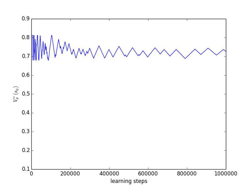
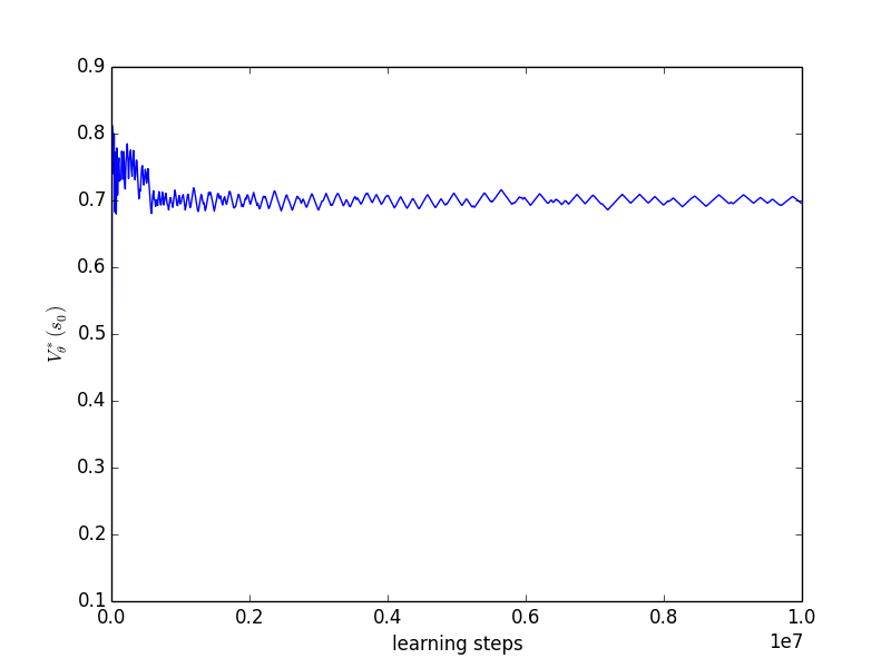
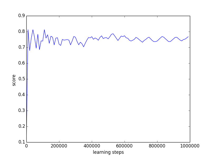
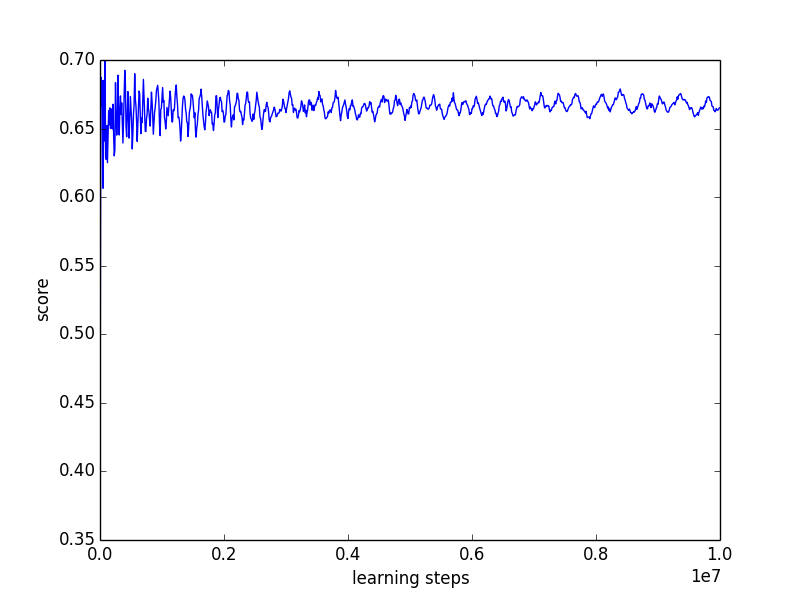
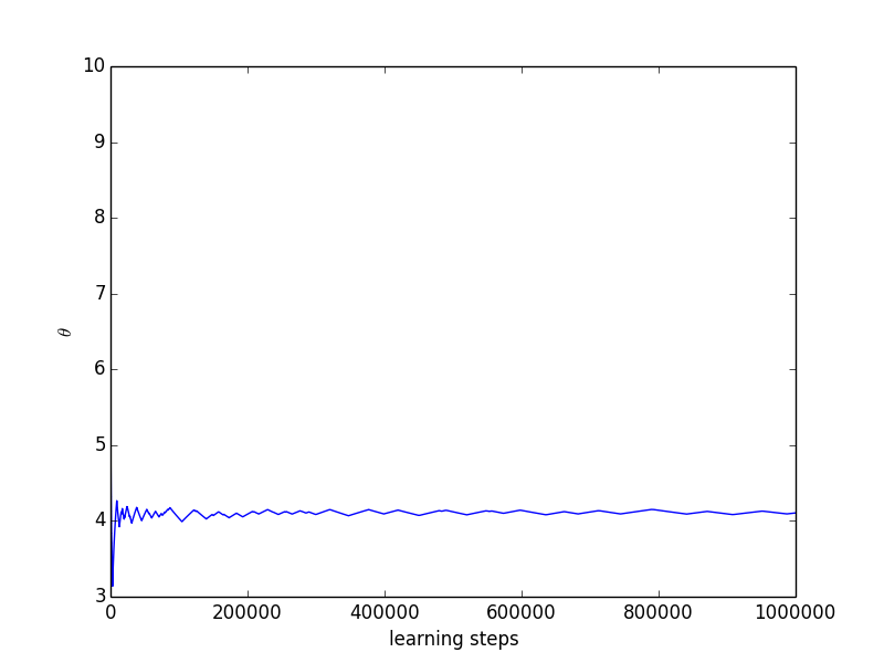
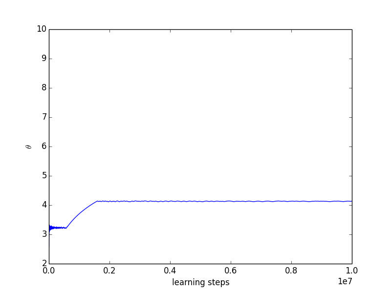
We plot the results (see Figure 1) obtained for two different learning runs, one with 1 million learning steps and the other with 10 million learning steps. The $\theta$-updates were interleaved with a Q-learning phase using an $\varepsilon$-greedy exploration strategy with $\varepsilon=0.01$ and with learning rate $\alpha(n)=1/(n+1)^{11/20}$. One can check that Equation 11 is satisfied. We optimize the upper quantile with $\tau=0.3$. During the learning process we maintain a vector $\mathbf{f}$ of frequencies with which each final state has been attained. We define the quantity score as the cross product between $\mathbf{f}$ and the vector of rewards obtained when attaining each final state given the current value of $\theta$. Put another way, score is the value of the non-stationary policy that has been played since the beginning of the learning process. Moreover, at each iteration we compute $V_{\theta}^{*}(s_{0})$, the optimal value in $s_{0}$ given the current value of $\theta$.

On Figures 1 and 1 we observe the evolution of $V_{\theta}^{*}(s_{0})$ as the number of iterations increases. We observe that $V_{\theta}^{*}(s_{0})$ converges towards $1-\tau=0.7$ as the number of iterations increases with oscillations of decreasing amplitude that are due to the ever changing $\theta$ value. Figures 1 and 1 show the evolution of the score as the number of iterations increases. Score converges towards a value of $0.7$ but inferior. This is due to the exploration of the Q-learning algorithm. Lastly, 1 and 1 plot the evolution of $\theta$ as the number of iteration increases. The value of $\theta$ converges towards a value of 4 which the one for which $V_{\theta}^{*}(s_{0})=1-\tau=0.7$.

References

- Abbeel et al. (2010) Pieter Abbeel, Adam Coates, and Andrew Y. Ng. Autonomous helicopter aerobatics through apprenticeship learning. International Journal of Robotics Research, 29(13):1608–1639, 2010.
- Akrour et al. (2012) R. Akrour, M. Schoenauer, and M. Sébag. April: Active preference-learning based reinforcement learning. In ECML PKDD, Lecture Notes in Computer Science, volume 7524, pages 116–131, 2012.
- Bäuerle and Ott (2011) Nicole Bäuerle and Jonathan Ott. Markov decision processes with average value-at-risk criteria. Mathematical Methods of Operations Research, 74(3):361–379, 2011.
- Benoit and Van den Poel (2009) D.F. Benoit and D. Van den Poel. Benefits of quantile regression for the analysis of customer lifetime value in a contractual setting: An application in financial services. Expert Systems with Applications, 36:10475–10484, 2009.
- Blackwell (1956) D. Blackwell. An analog of the minimax theorem for vector payoffs. Pacific Journal of Mathematics, 6(1):1–8, 1956.
- Borkar and Jain (2014) V. Borkar and Rahul Jain. Risk-constrained Markov decision processes. IEEE Transactions on Automatic Control, 59(9):2574–2579, 2014.
- Borkar (2008) Vivek S. Borkar. Stochastic approximation : a dynamical systems viewpoint. Cambridge university press New Delhi, Cambridge, 2008. ISBN 978-0-521-51592-4. URL http://opac.inria.fr/record=b1132816.
- Borkar (1997) V.S. Borkar. Stochastic approximation with time scales. Systems & Control Letters, 29(5):291–294, 1997.
- Boussard et al. (2010) M. Boussard, M. Bouzid, A.I. Mouaddib, R. Sabbadin, and P. Weng. Markov Decision Processes in Artificial Intelligence, chapter Non-Standard Criteria, pages 319–359. Wiley, 2010.
- Bruyère et al. (2014) Véronique Bruyère, Emmanuel Filiot, Mickael Randour, and Jean-François Raskin. Meet your expectations with guarantees: beyond worst-case synthesis in quantitative games. In STACS, 2014.
- Busa-Fekete et al. (2013) R. Busa-Fekete, B. Szörenyi, P. Weng, W. Cheng, and E. Hüllermeier. Preference-based reinforcement learning. In European Workshop on Reinforcement Learning, Dagstuhl Seminar, 2013.
- Busa-Fekete et al. (2014) Robert Busa-Fekete, Balazs Szorenyi, Paul Weng, Weiwei Cheng, and Eyke Hüllermeier. Preference-based Reinforcement Learning: Evolutionary Direct Policy Search using a Preference-based Racing Algorithm. Machine Learning, 97(3):327–351, 2014.
- Carpentier and Valko (2014) Alexandra Carpentier and Michal Valko. Extreme bandits. In NIPS, 2014.
- Chow and Ghavamzadeh (2014) Yinlam Chow and Mohammad Ghavamzadeh. Algorithms for cvar optimization in MDPs. In NIPS, 2014.
- DeCandia et al. (2007) G. DeCandia, D. Hastorun, M. Jampani, G. Kakulapati, A. Lakshman, A. Pilchin, S. Sivasubramanian, P. Vosshall, and W. Vogels. Dynamo: amazon’s highly available key-value store. ACM SIGOPS Operating Systems Review, 41(6):205–220, 2007.
- Delage and Mannor (2007) E. Delage and S. Mannor. Percentile optimization in uncertain Markov decision processes with application to efficient exploration. In ICML, pages 225–232, 2007.
- Fargier et al. (2011) Hélène Fargier, Gildas Jeantet, and Olivier Spanjaard. Resolute choice in sequential decision problems with multiple priors. In IJCAI, 2011.
- Filar (1983) Jerzy A. Filar. Percentiles and Markovian decision processes. Operations Research Letters, 2(1):13 – 15, 1983. ISSN 0167-6377. http://dx.doi.org/10.1016/0167-6377(83)90057-3. URL http://www.sciencedirect.com/science/article/pii/0167637783900573.
- Filar et al. (1989) Jerzy A. Filar, L. C. M. Kallenberg, and Huey-Miin Lee. Variance-penalized Markov decision processes. Mathematics of Operations Research, 14:147–161, 1989.
- Fishburn (1981) P.C. Fishburn. An axiomatic characterization of skew-symmetric bilinear functionals, with applications to utility theory. Economics Letters, 8(4):311–313, 1981.
- Fürnkranz et al. (2012) J. Fürnkranz, E. Hüllermeier, W. Cheng, and S.H. Park. Preference-based reinforcement learning: A formal framework and a policy iteration algorithm. Machine Learning, 89(1):123–156, 2012.
- Gilbert et al. (2015) Hugo Gilbert, Olivier Spanjaard, Paolo Viappiani, and Paul Weng. Solving MDPs with skew symmetric bilinear utility functions. In IJCAI, pages 1989–1995, 2015.
- Gilbert et al. (2016) Hugo Gilbert, Bruno Zanuttini, Paolo Viappiani, Paul Weng, and Esther Nicart. Model-free reinforcement learning with skew-symmetric bilinear utilities. In International Conference on Uncertainty in Artificial Intelligence (UAI), 2016.
- Gimbert (2007) Hugo Gimbert. Pure stationary optimal strategies in Markov decision processes. In STACS, 2007.
- Jaffray (1998) Jean-Yves Jaffray. Implementing resolute choice under uncertainty. In UAI, 1998.
- Jorion (2006) Philippe Jorion. Value-at-Risk: The New Benchmark for Managing Financial Risk. McGraw-Hill, 2006.
- Kalathil et al. (2014) D. Kalathil, V.S. Borkar, and R. Jain. A learning scheme for blackwell’s approachability in mdps and stackelberg stochastic games. Arxiv, 2014.
- Koenker (2005) R. Koenker. Quantile Regression. Cambridge university press, 2005.
- Liu and Koenig (2005) Y. Liu and S. Koenig. Risk-sensitive planning with one-switch utility functions: Value iteration. In AAAI, pages 993–999. AAAI, 2005.
- Liu and Koenig (2006) Y. Liu and S. Koenig. Functional value iteration for decision-theoretic planning with general utility functions. In AAAI, pages 1186–1193. AAAI, 2006.
- McClennen (1990) E. McClennen. Rationality and dynamic choice: Foundational explorations. Cambridge university press, 1990.
- Mnih et al. (2015) Volodymyr Mnih, Koray Kavukcuoglu, David Silver, Andrei A. Rusu, Joel Veness, Marc G. Bellemare, Alex Graves, Martin Riedmiller, Andreas K. Fidjeland, Georg Ostrovski, Stig Petersen, Charles Beattie, Amir Sadik, Ioannis Antonoglou, Helen King, Dharshan Kumaran, Daan Wierstra, Shane Legg, and Demis Hassabis. Human-level control through deep reinforcement learning. Nature, 518:529–533, 2015.
- Ng and Russell (2000) A.Y. Ng and S. Russell. Algorithms for inverse reinforcement learning. In ICML. Morgan Kaufmann, 2000.
- Perea and Puerto (2007) F. Perea and J. Puerto. Dynamic programming analysis of the TV game who wants to be a millionaire? European Journal of Operational Research, 183(2):805 – 811, 2007. ISSN 0377-2217. http://dx.doi.org/10.1016/j.ejor.2006.10.041. URL http://www.sciencedirect.com/science/article/pii/S0377221706010320.
- Puterman (1994) M.L. Puterman. Markov decision processes: discrete stochastic dynamic programming. Wiley, 1994.
- Randour et al. (2014) Mickael Randour, Jean-François Raskin, and Ocan Sankur. Percentile queries in multi-dimensional Markov decision processes. CoRR, abs/1410.4801, 2014. URL http://arxiv.org/abs/1410.4801.
- Regan and Boutilier (2009) K. Regan and C. Boutilier. Regret based reward elicitation for Markov decision processes. In UAI, pages 444–451. Morgan Kaufmann, 2009.
- Rostek (2010) M.J. Rostek. Quantile maximization in decision theory. Review of Economic Studies, 77(1):339–371, 2010.
- Szörényi et al. (2015) Balázs Szörényi, Róbert Busa-Fekete, Paul Weng, and Eyke Hüllermeier. Qualitative multi-armed bandits: A quantile-based approach. In ICML, pages 1660–1668, 2015.
- Tesauro (1995) Gerald Tesauro. Temporal difference learning and td-gammon. Communications of the ACM, 38(3):58–68, 1995.
- Weng (2011) P. Weng. Markov decision processes with ordinal rewards: Reference point-based preferences. In ICAPS, volume 21, pages 282–289. AAAI, 2011.
- Weng (2012) P. Weng. Ordinal decision models for Markov decision processes. In ECAI, volume 20, pages 828–833. IOS Press, 2012.
- Weng and Zanuttini (2013) P. Weng and B. Zanuttini. Interactive value iteration for Markov decision processes with unknown rewards. In IJCAI, 2013.
- White (1987) D. J. White. Utility, probabilistic constraints, mean and variance of discounted rewards in Markov decision processes. OR Spektrum, 9:13–22, 1987.
- Wolski and Brevik (2014) R. Wolski and J. Brevik. QPRED: Using quantile predictions to improve power usage for private clouds. Technical report, UCSB, 2014.
- Yu and Nikolova (2013) Jia Yuan Yu and Evdokia Nikolova. Sample complexity of risk-averse bandit-arm selection. In IJCAI, 2013.
- Yu et al. (1998) Stella X. Yu, Yuanlie Lin, and Pingfan Yan. Optimization models for the first arrival target distribution function in discrete time. Journal of mathematical analysis and applications, 225:193–223, 1998.
- Zhang et al. (2001) B. Zhang, Q. Cai, J. Mao, E Chang, and B. Guo. Spoken dialogue management as planning and acting under uncertainty. In 7th European Conference on Speech Communication and Technology, 2001.