Quantitative Evaluation of Hardware Binary Stochastic Neurons
Abstract
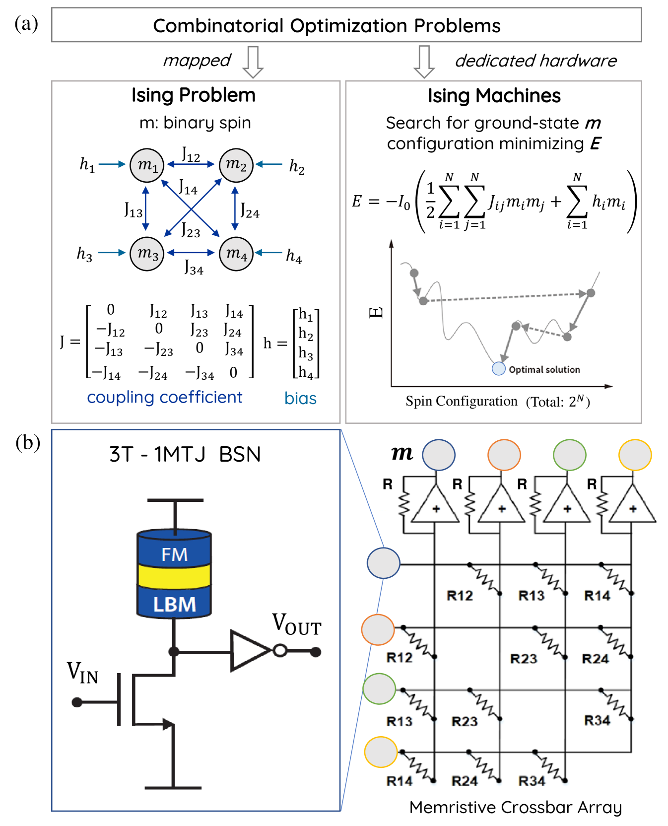
Recently there has been increasing activity to build dedicated Ising Machines to accelerate the solution of combinatorial optimization problems by expressing these problems as a ground-state search of the Ising model. A common theme of such Ising Machines is to tailor the physics of underlying hardware to the mathematics of the Ising model to improve some aspect of performance that is measured in speed to solution, energy consumption per solution or area footprint of the adopted hardware. One such approach to build an Ising spin, or a binary stochastic neuron (BSN), is a compact mixed-signal unit based on a low-barrier nanomagnet based design that uses a single magnetic tunnel junction (MTJ) and three transistors (3T-1MTJ) where the MTJ functions as a stochastic resistor (1SR). Such a compact unit can drastically reduce the area footprint of BSNs while promising massive scalability by leveraging the existing Magnetic RAM (MRAM) technology that has integrated 1T-1MTJ cells in Gbit densities. The 3T-1SR design however can be realized using different materials or devices that provide naturally fluctuating resistances. Extending previous work, we evaluate hardware BSNs from this general perspective by classifying necessary and sufficient conditions to design a fast and energy-efficient BSN that can be used in scaled Ising Machine implementations. We connect our device analysis to systems-level metrics by emphasizing hardware-independent figures-of-merit such as flips per second and dissipated energy per random bit that can be used to classify any Ising Machine.
I Introduction
In the era of internet of things (IoT), combinatorial optimization problems are ubiquitous Yamaoka et al. (2015). In fact, most of the real-problems that quantum computers are aiming to solve can be formulated as combinatorial optimization problems.From directing traffic flow Neukart et al. (2017), to routing interconnections in integrated circuit design Barahona et al. (1988); Cook et al. (2018), to making financial decisions Rosenberg et al. (2016), drug discoveries Sakaguchi et al. (2016), etc. - all involve solving a form of combinatorial optimization problems. The demand for solving these problems faster and more efficiently is ever-increasing. But such problems typically fall into the category of NP-hard or NP-complete class in complexity theory Barahona (1982), with no known polynomial time solution, making them notoriously difficult to solve in digital computers using traditional computing methods. This has given rise to a new paradigm in computing, namely Ising computing. Ising computing maps combinatorial optimization problems to an Ising model, and solves it by searching for the ground state of the system described by Lucas (2014); Sutton et al. (2017):
| (1) |
where, denotes the Ising spin, is the coupling co-efficient, is the external bias, and is the annealing parameter which is proportional to the inverse of temperature. In the machine learning field, the same underlying principle is used for Boltzmann Machines with the annealing parameter being 1. The binary stochastic neurons (BSNs) BSN of stochastic neural networks are well suited to function as a ‘spin’ is such systems, described mathematically by:
| (2) |
where is a random number between and , and is the input to the neuron.
Given the importance of optimization problems, a lot of research has gone into developing algorithms and identifying appropriate hardware for Ising computing. Various approaches including quantum computers based on quantum annealing (QA) or adiabatic quantum optimization (AQC) implemented with superconducting circuits Johnson et al. (2011), coherent Ising machines (CIMs) implemented with laser pulses McMahon et al. (2016), phase-change oscillators Dutta et al. (2020), or CMOS oscillators Goto, Tatsumura, and Dixon (2019); Wang and Roychowdhury (2019); Ahmed, Chiu, and Kim (2020); Chou et al. (2019) and digital annealers based on simulated annealing (SA) Kirkpatrick, Gelatt, and Vecchi (1983) implemented with digital circuits Baity-Jesi et al. (2014); Yamaoka et al. (2015); Takemoto et al. (2019); Aramon et al. (2019); Yamamoto et al. (2020); Patel et al. (2020); Patel, Canoza, and Salahuddin (2020) are being explored.
In this paper we comprehensively evaluate and characterize a stochastic magnetic tunnel junction (sMTJ) based realization of the Ising spin (eqn.2) where random numbers are generated using the natural physics of low barrier nanomagnets Camsari, Salahuddin, and Datta (2017) in a compact design. A network of these BSN units can be coupled with a memristive crossbar array Xia et al. (2016); Cai et al. (2019a); Bayat et al. (2018) to perform the synaptic operation as shown in Fig. 1 can drastically improve the area requirements and accelerate computation speed of Ising Machines. We evaluate the performance of the BSN device in terms of its energy and delay metrics and connect these to the problem and substrate-independent metric of flips per second that the probabilistic system makes Sutton et al. (2019).
Our evaluation of 1MTJ-3T BSN design considers different types of low-barrier nanomagnet realizations of MTJs. As the MTJ essentially functions as a two-terminal stochastic resistor (SR), we first take a general 3T-1SR design approach, classifying necessary and sufficient conditions for achieving the BSN operation for different types of SRs in Section II. We relate these conditions to the different sMTJ realizations in Section III. We report the timescale of operation, power and energy for each case based on benchmarked SPICE simulations of the BSN hardware consisting of spintronic elements from a modular circuit framework Torunbalci et al. (2018) coupled to 14 nm FinFET PTM models pre , and provide analytical results for relevant quantities in Section IV. Lastly, we use these device performance metrics to project onto hardware performance figures of merit such as flips per second that a probabilistic sampler makes. Our projections indicate orders of magnitude improvement potential over current digital implementations.
II General Approach to Design of BSN
Binary stochastic neurons (BSNs) are well suited to function as a ‘spin’ in Ising machines for solving combinatorial optimization problems BSN ; Hassan et al. (2019). A compact and efficient hardware realization of the BSN leveraging the natural physics of stochastic nanomagnets can be made by using unstable magnetic tunnel junctions (MTJs) Daniels et al. (2020); Parks et al. (2018); Grollier et al. (2020); Abeed and Bandyopadhyay (2019); Drobitch and Bandyopadhyay (2019) as shown in Fig. 1.
The compact design of BSN based on low-barrier magnet (LBM) stochastic MTJs (sMTJs) was first proposed in 2017 Camsari, Salahuddin, and Datta (2017). Using magnet and circuit physics to analyze the performance, it was reported that using an LBM in a circular disk geometry with energy barriers below as the free layer of an MTJ results in sub-ns response times requiring only a few fJ of energy per random bit Hassan et al. (2019). The proposed design and the performance analysis considers a very specific type of sMTJ which had circular in-plane magnetic anisotropy (IMA) whose fluctuations are undisturbed by the current in the circuit for typical current drive conditions. However, in 2019, a version of the BSN design that was implemented in hardware to solve an 8-bit factorization problem Borders et al. (2019), consisted of an sMTJ with perpendicular anisotropy (PMA) and a barrier of a few as its free layer. Unlike the circular in-plane design, the PMA design relied on its resistance being tunable by the spin-transfer-torque effect in order to achieve the BSN operation. This has called for an extension of our initial analysis presented in Hassan et al. (2019) which we systematically perform in this paper.
As the MTJs in the BSN circuit effectively act as a fluctuating resistor, Parks et al. (2020) and the design principle is independent of this realization, for establishing the fundamental design rules we approach it from a general perspective and we hope these design rules stimulate discussion in the realization of different stochastic resistors that use different mechanisms Cheemalavagu et al. (2005); Shukla et al. (2014); Kumar, Strachan, and Williams (2017); Stampfer et al. (2018); Cai et al. (2019b); Camsari et al. (2020).
II.1 Types of fluctuating resistances
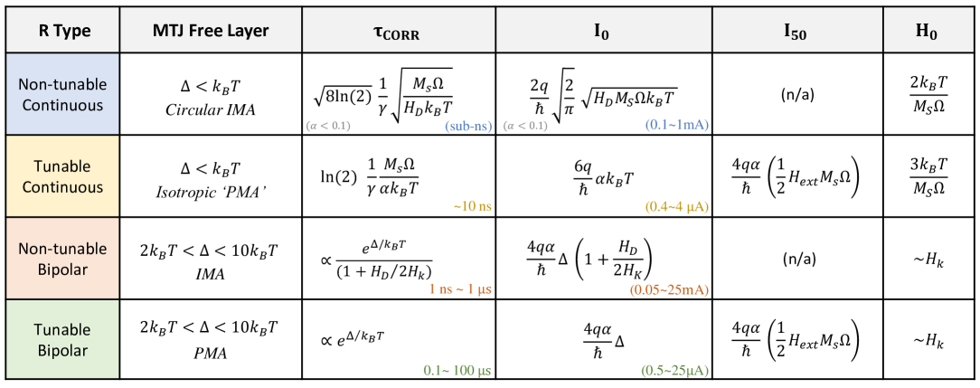
We categorize the fluctuating into four types. First, based on the fluctuating nature it can be continuous or bipolar (telegraphic). Second, it can be tunable or non-tunable depending on whether it is affected by the current that is flowing through it.
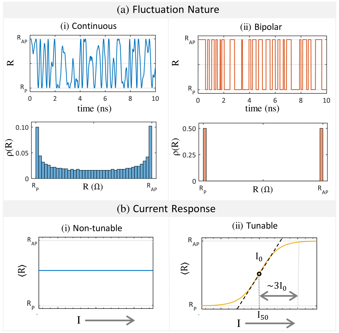
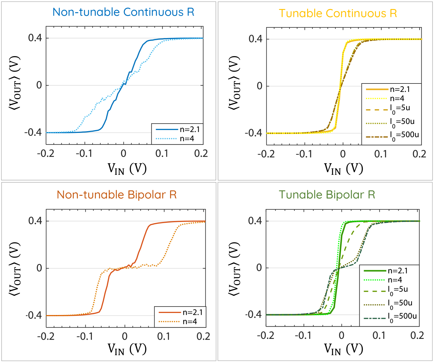
A continuous resistor can have its resistance being any value between while a bipolar resistor only assumes the two values and as shown in Fig. 2(a). The distribution of continuous resistances can be of different types as well. It can be uniform or follow slightly bimodal distribution in the case of an MTJ as shown in the figure. Different distributions typically result in different average values, slightly bimodal or uniform distributions are better suited than Gaussian distributions for BSN realizations.
The current flowing in the circuit can tune the probability distribution of the resistance fluctuations, and we call such resistors tunable resistors. When designing a BSN with current tunable R, we need to know the current where fluctuations are equal between the two extreme states () Parks et al. (2020) and the current required to pin the resistance to one of those states. An important parameter in this case is the bias current , which is the slope of the curve at the 50-50 point. Typically, current is required to pin the fluctuating resistance to one of its states. We will later provide analytical expressions for for four cases of resistors that can be obtained by various MTJs (Fig. 9).
Based on this analysis, we categorize the fluctuating resistance into four types: Non-tunable continuous (NTC), Non-tunable bipolar (NTB), tunable continuous (TC) and tunable bipolar (TB).
II.2 Performing the BSN function
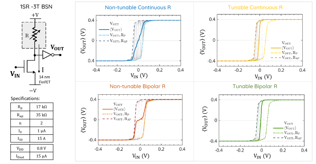
We first take a look at the transfer characteristics of the device to see whether the four types of resistance can faithfully mimic BSN operation described by eqn.2. The fluctuating is a physical realization of the random variable , the NMOS acts as a constant current source that provides tunability, and the inverter performs the operation in eqn.2.
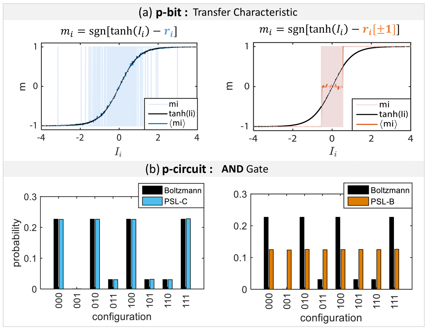
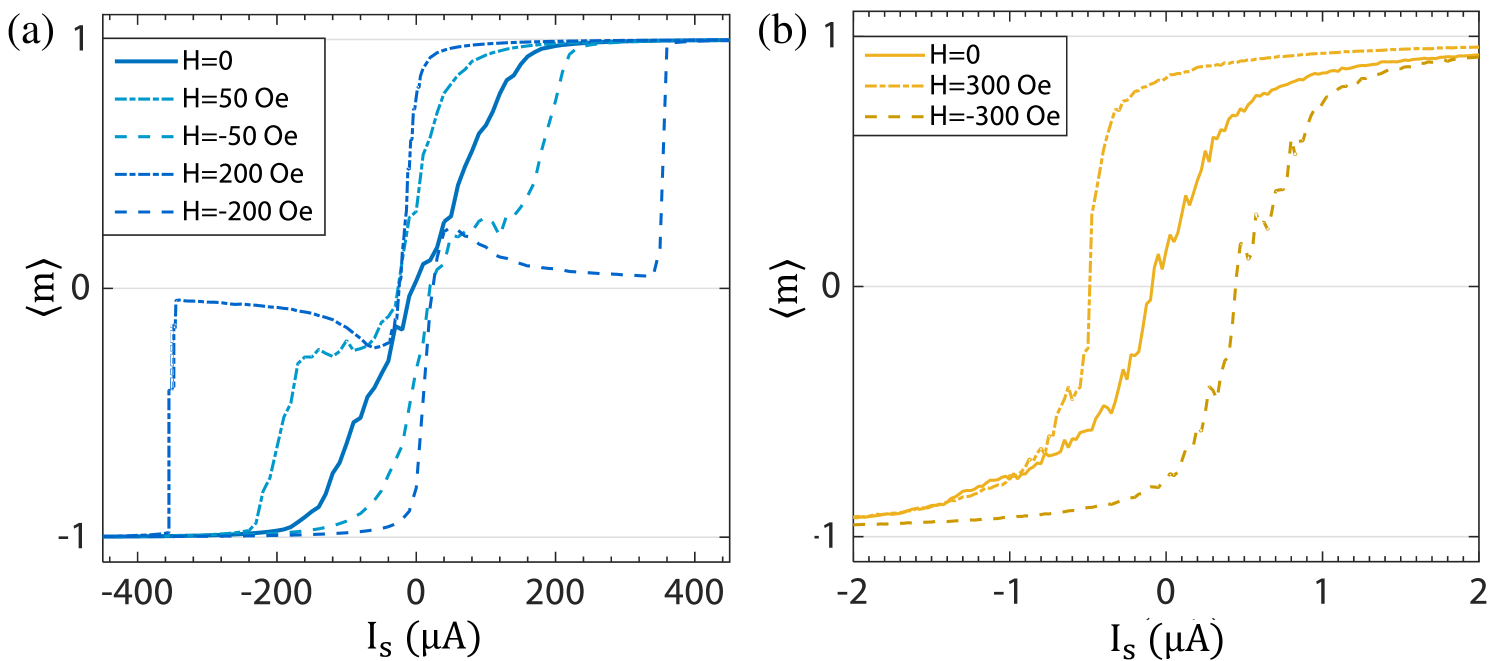
Fig. 3, shows that while all other resistance types were able to reproduce the desired sigmoidal average curve , the non-tunable bipolar resistor gives a staircase-like function instead. This is because of the fixed delta function like resistance distribution at the two extreme states (see Fig. 2(a)ii. As there is no continuity in the resistance distribution and no additional means of tuning the delta distribution itself has been introduced to the structure, the BSN output fluctuations are equal until either of the threshold points are crossed, resulting in the stair-case like function.
Mathematically, when the resistance is bipolar, it means is . So, for any input where , the output is equal to zero. In fig. 4(b), if we look at a simple invertible AND gate Camsari et al. (2017); Camsari, Salahuddin, and Datta (2017) operation, it is seen that devices with stair-case like function like this are not suitable for performing as BSNs. This has been demonstrated experimentally in ref.Lv, Bloom, and Wang (2019); Zink, Lv, and Wang (2019) where a stable MTJ was used as a bipolar resistor whose distribution was tuned by an external field. However, this issue could be resolved by introducing external/additional control parameters like external field as shown in the same experiment.
II.3 Parameter Dependence and Design Choices
Fig. 3 is created with a fixed set of parameters for the resistor and coupled with a specific transistor technology, 14 nm FinFET models. In this section we explore how the transfer characteristics are affected by different parameters of the resistors and FET characteristics and how to choose the right combination of and FET to be coupled.
Stochastic Region: The stochastic region, which we define next, is a function of the resistance ratio for non-tunable resistors and biasing current for tunable resistors as shown in Fig.5, that needs to be matched with the transistor characteristics.
Effect of n: The resistance ratio is directly related to the stochastic region through the NMOS characteristics in case of non-tunable resistor designs. The edge of the stochastic region is defined by when where the current is determined by the NMOS as shown in Fig. 6(c). For a desired (stochastic region) and NMOS transistor, the required should approximately equal . Ideally, the minimum value of the resistance should be and to get full pinning, should be less than . For a 14 nm FinFET, to get a stochastic region of , the resistance ratio should be around . The resistance ratio is a measure for tunneling magneto-resistance, TMR () in case of MTJs. For the non-tunable case, TMR needs to be large enough to provide a voltage swing large enough to overcome the noise margins of the inverter Hassan et al. (2019), and it should be small enough so that output pinning is achieved within the given input range. Typically MTJs have TMRs ranging from Parkin et al. (2004) with a maximum reported TMR of Ikeda et al. (2008), so the resistance ratio of MTJs are well within the desired range, but the general requirements we outline should be applicable for other types of stochastic resistors as well.
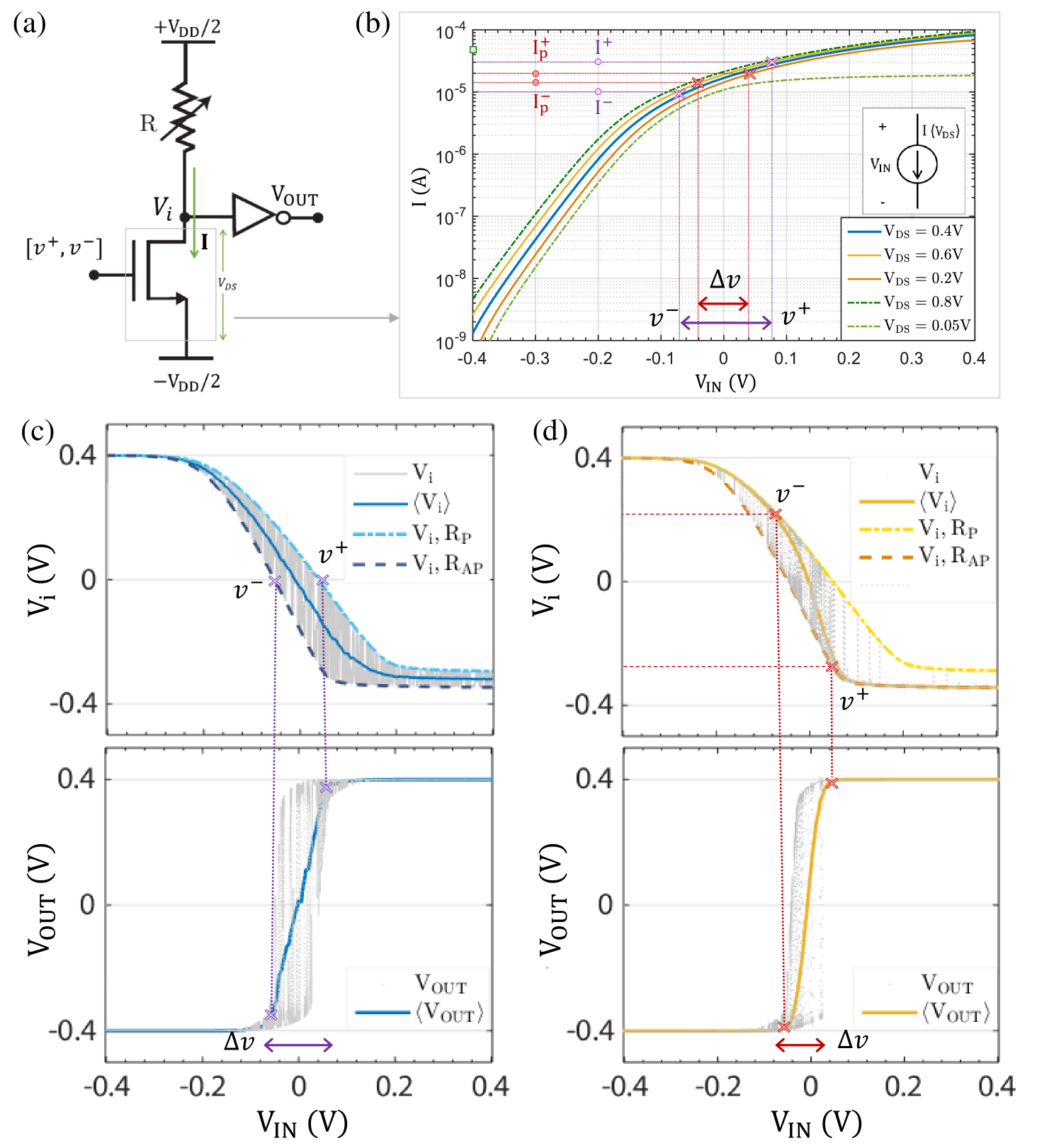
Effect of : In case of tunable resistances, the stochastic region is independent of the resistance ratio and depends on the pinning current and thus the bias current () instead as shown in Fig. 6(d). For large bias currents (), the tunable resistances act essentially like non-tunable resistances. To get the full range of R,the NMOS needs to be able to supply the pinning current. If the pinning current is as shown in Fig. 2, then to get the full range of the resistance needs to be around . In case of 14 nm FinFETs, is around , restricting to values less than .
Choice of : Another parameter that is important for the operation of tunable resistors is the which determines the midpoint of the sigmoid. is the current at which the resistance on average spends equal time in and states Parks et al. (2020). As the circuit can only support positive current values, it needs to be a positive quantity and preferably matched with the saturation point () current of the NMOS transistor. Changing shifts the transfer characteristics laterally as shown in Fig. 7(a).
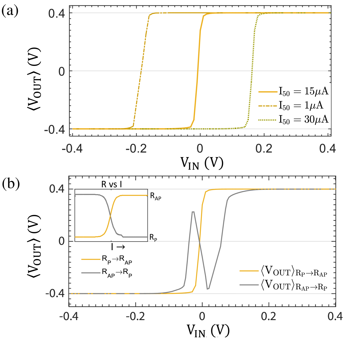
R vs I: One last requirement is that, for current tunable resistance with increasing current , the resistance needs to increase from . This can be understood intuitively: Increasing means the NMOS transistor is becoming more conductive. If the MTJ concomitantly becomes more conductive as is increasing, the transfer characteristics can show non-monotonic behavior as shown in Fig. 7(b). This requirement holds true irrespective of whether the circuit’s branch consists of a PMOS-1R or 1R-NMOS topology.
III Realization of fluctuating resistances with sMTJs
A magnetic-tunnel-junction (MTJ) whose free layer is a low-barrier magnet (LBM) could serve as a physical realization of fluctuating resistors. Depending on the nature and characteristics of the LBM magnetization fluctuations, we can get different types of R. Our previous analysis Hassan et al. (2019) was restricted to one type of LBM, the circular IMA with barrier , in this section we extend it to include all possible LBMs.
A general description of the energy associated with a magnet is given by Hassan et al. (2019):
| (3) | ||||
where, is the perpendicular anisotropy field along the x-axis, is the surface anisotropy density, is the in-plane anisotropy along z-axis, is the external field, is the saturation magnetization and is the volume of the magnet. By adjusting the thickness or the shape of the magnet, the magnetic anisotropy of the magnet can be scaled to behave like a low-barrier magnet Debashis et al. (2018); Hassan et al. (2019).Second order magnetic anisotropy effect and in-plane components of demagnetization fields have not been considered here and left for future investigation since the macroscopic models without it seems to be reasonably consistent with recent experimental results involving low barrier magnets Debashis et al. (2016); Safranski et al. (2020); Parks et al. (2020); Zhang et al. (2021). We use the stochastic LLG module from our spintronics library nanohub.org to simulate the LBM dynamics in HSPICE using its transient noise function. This model has been carefully benchmarked against general Fokker-Planck based methods Torunbalci et al. (2018).
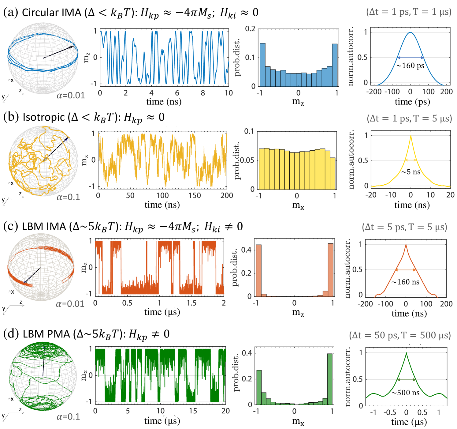
magnets have more continuous fluctuations with (b) having a more uniform distribution than (a) while slightly higher barrier magnets have a more telegraphic fluctuation. In both cases, the presence of high demagnetization fields cause faster fluctuations in IMA magnets.
LBM Magnet Fluctuation Dynamics: By low-barrier magnet we refer to magnets whose barrier is or so, whose magnetization fluctuates randomly in presence of thermal noise. Interestingly, the magnetization dynamics of low-barrier magnets with barrier are different from those with a slightly higher barrier Hassan et al. (2019); Kaiser et al. (2019). The simple exponential dependence of retention time of the magnetization state on the barrier height is not valid around or below Coffey and Kalmykov (2012).
Fig. 8 shows the fluctuation dynamics, the magnetization distribution, and the auto-correlation time () for low barrier magnets. Magnetization fluctuations translate into resistance fluctuations in MTJ, and we see that magnets with barrier act like continuous resistances, while slightly higher barrier magnets, which have a more defined two states, give telegraphic fluctuations, and in both cases IMA magnets fluctuate orders of magnitude faster than their PMA counterparts due to a novel mechanism where the demagnetization field plays a central role Pufall et al. (2004); Safranski et al. (2020); Hassan et al. (2019); Kaiser et al. (2019); Faria, Camsari, and Datta (2017).
Current Response of LBM Magnets: Magnetic fluctuations can be tuned by spin-current. For high barrier magnets, the minimum current required to switch the magnetization is called the critical current Sun (2000), in case of low-barrier magnets, we refer to it as a biasing current, defined by the inverse of the derivative taken at , mathematically expressed as: at low bias (). The current required to pin the magnetization, similar to switching current in high-barrier magnets is assumed to be , as indicated in Fig. 2. IMA magnets have a much larger pinning current than PMA magnets because of the large demagnetization field present due to their disk shape Hassan et al. (2019); Sun (2000); Faria, Camsari, and Datta (2018), meaning transistors with much larger current ranges would be required for IMA magnet MTJs than PMA for tunable resistors.
An important thing to note here is the current tunability in presence of an external field which can arise, for example, due to the fixed, stable layer that acts as a reference to the free layer in the MTJ. In the case of high-barrier magnets, the spin-current induced magnetic switching hysteresis loop just shifts in case of PMA magnets depending on the direction of field, but for IMA magnets the shape of the hysteresis and magnet dynamics is changed Sun (2000). The large demagnetizing field present perpendicular to the magnetization plane in IMA magnets causes the magnetization to precess around it when spin-current is applied in the opposite direction to the external field. The same is observed in low-barrier magnets as shown in Fig. 10. The larger the external field the more pronounced the effect is. The uniform precessional motion kicks in at high-field, when the current is close to the biasing current or higher applied in the opposite direction to the field. Very recently, this has been observed experimentally for low fields Safranski et al. (2020). While this is an undesired effect in case of our BSN operation, this can be useful in context to oscillator based networks Romera et al. (2018).
This has important implications in terms of acting as a fluctuating resistance in a BSN circuit. IMA magnets with external fields (i.e. uncompensated dipolar fields in MTJ Jenkins et al. (2019)) greater than its pinning field is not suited to function as a tunable or non-tunable resistor. IMA magnets with continuous magnetization coupled to a transistor with small saturation current () compared to the biasing current of IMA () can work as non-tunable resistors, and as experimental observations in ref. Safranski et al. (2020) suggest, it can withstand small (compared to its pinning field) stray fields.
PMA magnet MTJs with their small biasing current ( few to few tens of ) when coupled to typical transistors act as tunable resistors in BSN circuit. In this case the external bias field is actually preferred, since this enables positive current Borders et al. (2019).
IV Performance Evaluation of MTJ based BSN
In the final section we compare the physical performance of these different sMTJs in a BSN.
Timescale of Operation: The two relevant timescales of operation for a BSN are, the correlation time which is the average time it takes to produce a new output at given input and the response time which is defined as the average time it takes for the circuit to give a random output with correct statistics as the input is changed Hassan et al. (2019). Fig. 11 shows the two timescales for the three types of fluctuating resistances for MTJs with two different timescales. For simplicity we assumed the correlation time to be same for all types of magnets, but in reality they would follow the relations indicated in Fig. 9 Kaiser et al. (2019); Hassan et al. (2019).
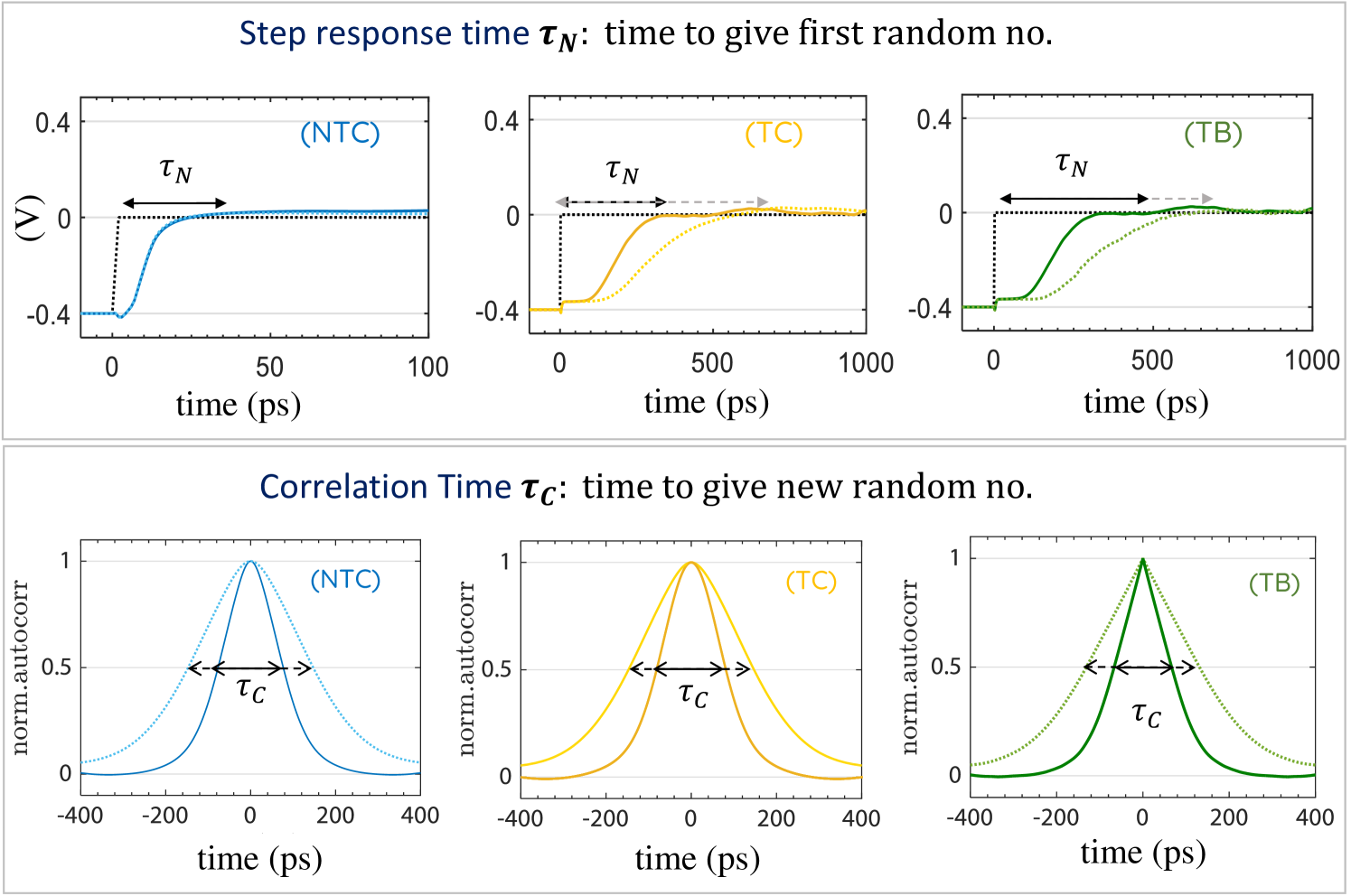
Fig. 11 shows that the response time, for non-tunable resistor is independent of the fluctuation time of the resistance, it is rather proportional to the RC delay of the circuit. While for the tunable cases, the response time is related to the characteristic timescales of the resistor. But the time to give new numbers or flip rate at is entirely resistance fluctuation time dependent for all cases (). So for the tunable case, the two said timescales of operation are likely to be similar as they are governed by the magnet fluctuation characteristics while for the non-tunable case, the response time which is RC dependent has the potential to be very short compared to the magnet dependent correlation time. For most applications this difference may not be of importance but for some applications where the network is directed, like Bayesian inference having two different timescales seems to be a requisite Faria et al. (2020).
Power: Our SPICE simulations indicate that the average power consumed by the BSN circuit in its stochastic region is Hassan et al. (2019). The is for the two branches, the MTJ branch and the inverter branch. This holds true for all types of resistors. For a 14 nm FinFET with and , . While the power is almost independent of TMR or the resistance ratio (n) for a set 50-50 point and technology for the MTJ branch, its joule heating increases with increasing TMR () in the positive pinning region as the NMOS resistance reduces. So the lowest TMR that ensures a voltage swing greater than the noise margin of the inverter is considered best suited for BSN operation. The MTJ branch power could be reduced by operating in subthreshold region , but this reduces the total power by while trading-off with an increase in the RC response time. Given the flexibility, it is preferable to design the MTJ to operate in the saturation region of transistor. For tunable case this means matching , for non-tunable this means having .
Energy: As there are two timescales associated with the BSN operation, we can define two energy as well. The energy to produce first random number after the input changes, and the energy required to produce new random numbers at a given input state, . Fig. 12(a) shows an energy delay plot indicating the ranges for each type of MTJs. When describing the performance of a hardware BSN, we generally refer to the correlation time for delay and for the energy. The individual energy-delay numbers can be used to project performance parameters for processors built with them.
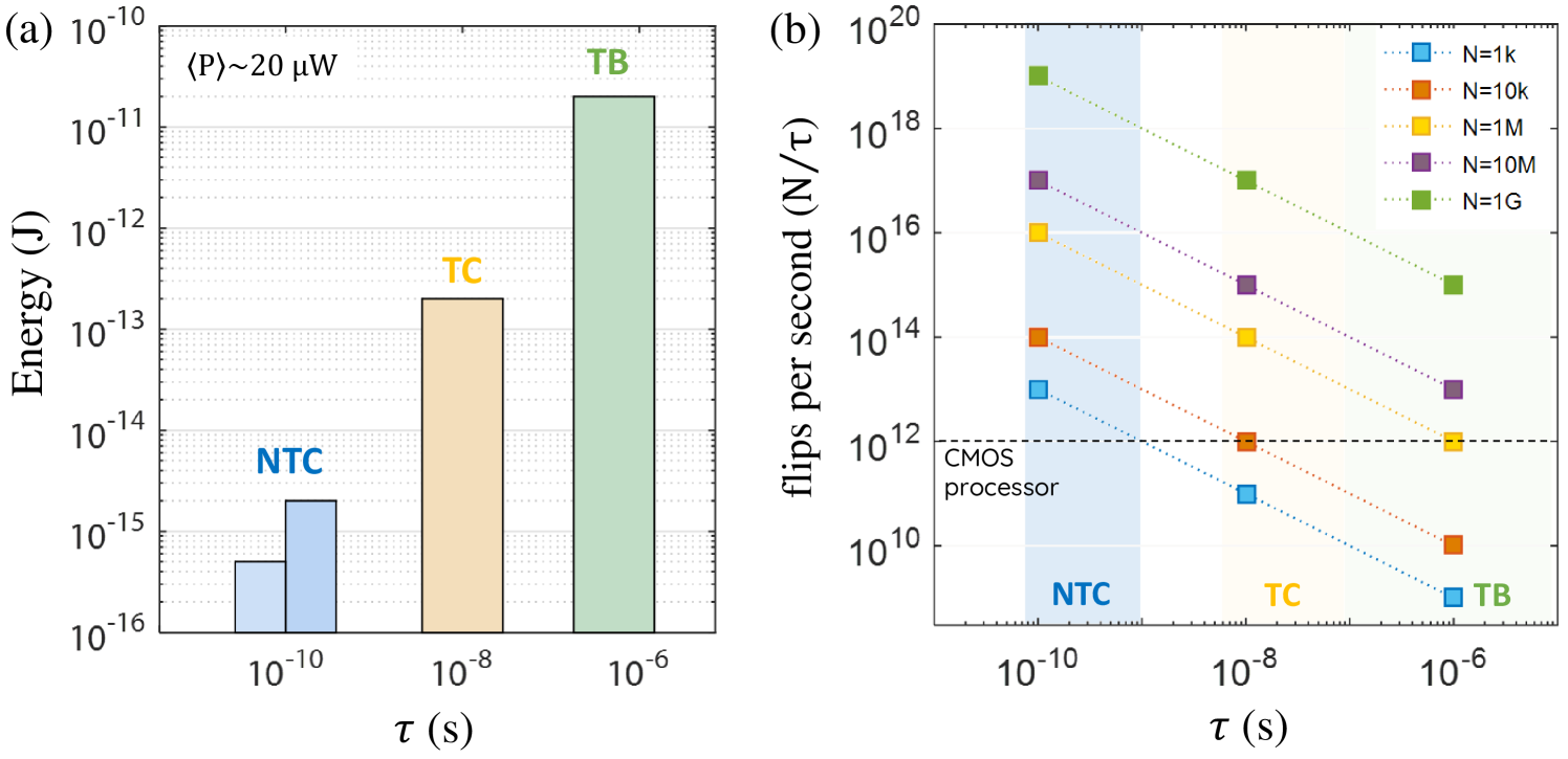
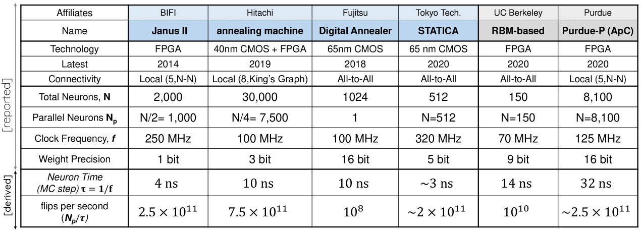
Hardware Projections: Typically the performance of an Ising hardware is measured in terms of time and energy it takes to solve a specific problem. Time to solution depends not only on the physical hardware performance but also on the algorithm that is being implemented. Here, we emphasize measuring the hardware performance in terms of a purely hardware metric flips per second (fps) Sutton et al. (2019); Isakov et al. (2015); Baity-Jesi et al. (2014), which refers to the maximum number of spin configurations the hardware can cycle through per second. It depends on the number of spins in the system (N) and the time it takes for a spin to flip (), .
For the digital annealers the spin update time is usually determined by its clock period () which ranges typically in tens of ns range. To ensure fidelity simultaneous updates of connected spins needs to be avoided Aarts, Aarts, and Lenstra (2003) forcing digital annealers that operate on clock edge to update spins sequentially. So in a network where all spins are connected effectively only one spin can update per clock cycle Aramon et al. (2019). But it need not be if some spins are unconnected (i.e. nearest neighbor Yamaoka et al. (2015); Baity-Jesi et al. (2014), or king-graph Takemoto et al. (2019) connection, or if spins are parallelized by implementing special algorithms Yamamoto et al. (2020); Patel et al. (2020); Patel, Canoza, and Salahuddin (2020). Based on the reported total spin number and clock speeds of digital annealing hardware today which have about neurons that can update per clock period, we derive an estimation of their performance at flips per second Yamaoka et al. (2015); Sutton et al. (2019) as shown in Fig. 13.
Compared to digital annealers the Ising spin hardware we presented in this work can work autonomously, i.e, without a synchronizing clock or a sequencer Sutton et al. (2019); Faria et al. (2020); Kaiser et al. (2020). In this mode, the speeds are governed by neuron () and synapse () time only, and to ensure fidelity and avoid simultaneous updates of connected BSNs the synapse needs to update faster than the the neuron (). Sutton et. al.Sutton et al. (2019) defines a metric and showed that to ensure the fidelity of operations needs to be less than 1. The exact requirements are problem and architecture dependent. Memristive crossbar arrays paired with a fast summing amplifier synapse could operate very efficiently at as low as few tens of ps speeds Xia et al. (2016); Cai et al. (2019c); Huang et al. (2015); Bayat et al. (2018); Hu et al. (2018); Cai et al. (2019a).
The digital annealers mimic the Ising spin using a combination of random-number generators (LFSR, Xoshiro, etc.), look-up-tables (LUT) and comparators. The random number generator (RNG) unit is one of the most are expensive elements in the design Gyoten, Hiromoto, and Sato (2018). Even in the most optimized design, the RNG unit take up of the total logic gate area Yamamoto et al. (2020). The 3T-1MTJ design offers drastic reduction in the area footprint, promising massive scalability leveraging existing 1T-1MTJ Magnetic RAM technology that already has 1Gbit integrated cells Aggarwal et al. (2019); eve (2019).
Fig. 12(b) projects fps number considering for different no of spins, N. An MTJ realization with circular IMA, with ns timescale can offer almost two orders of magnitude speedup with neurons. If spins are implemented in Gbit densities all stochastic implementations seem to outperform the CMOS implementations. For such systems the upper bound for N is ultimately determined either by area or by power budget of the chip. Note that the fps number does not reflect the connectivity of the spins or the algorithm implemented by the hardware. It also does not indicate the solution accuracy obtainable for specific problems Zhang et al. (2020). What we highlight here is that using the natural physics of the MTJ we can design a very compact realization of eq. 2 compared to current state of the art CMOS implementations, and despite being a magnetic circuit, low barrier magnet implementations even offer an overall speed up due to their fast fluctuation rates.
V Conclusion
In this paper, we presented a comprehensive evaluation of naturally stochastic magnetic building blocks for implementing probabilistic algorithms compactly and efficiently. We generalized the proposed 1MTJ-3T design to a 1SR-3T design and presented necessary design rules for BSN operation that we hope will stimulate further interest in finding stochastic resistance (1SR) with suitable properties. We extended the physical performance analysis of the 1MTJ-3T BSN design to include unstable MTJ’s with different low-barrier-magnets as free layers. They are evaluated as physical realizations of the general stochastic resistor (SR) with respect to 14 nm FinFET transistors. IMA magnets with barrier proved to be the best option, low-barrier PMA can function as current-tunable resistors as well. While careful optimization of the fixed layer to cancel the stray fields in IMA MTJ is preferred, PMA can benefit from the presence of stray fields (can be a source of the ). The most challenging set of working conditions are set for telegraphic IMA magnets, even if they are highly optimized and no stray fields are present in the circuit, they need to be coupled with high current transistors due to their high pinning currents, because if paired with low current transistors like 14 nm FinFET results in a staircase-like functional behavior which does not work as a p-bit as we discussed.
These BSNs are an integral part of Ising machines which are often referred to as annealing processors. Using 1MTJ-3T BSN could speed up the operation of these processors by orders of magnitude. Another important application space for these BSN is stochastic neural networks Kaiser et al. (2020); Nasrin et al. (2019); Schuman et al. (2017); Hinton (2002). In fact, binary stochastic neurons are desired for deep learning networks, but are typically avoided because it is harder to generate random bits in CMOS hardware Courbariaux et al. (2016). Use of this compact neuron that relies on MTJs natural physics to provide stochastic binarization could accelerate computation in custom hardware Tsai et al. (2017); Park et al. (2015) by faster evaluation of BSN function Hassan et al. (2019) and also encourage algorithmic advancement using BSN.
Acknowledgements.
This work was supported by the Center for Probabilistic Spin Logic for Low-Energy Boolean and Non-Boolean Computing (CAPSL), one of the Nanoelectronic Computing Research (nCORE) Centers as task 2759.005, a Semiconductor Research Corporation (SRC) program sponsored by the NSF through CCF 1739635.Appendix A Derivation for Pinning Field of LBM
Magnets are generally used to store information putting the focus on the evaluating and predicting characteristics of stable high-barrier magnets. It is interesting to note that theoretical predictions and analytical derivations regarding low-barrier magnet () dynamics typically receive less attention as cases of ’least practical interest’Brown Jr (1963). We document the analytical expressions associated with LBM in Fig. 9. The expressions for correlation time and biasing current can be found in ref.Coffey and Kalmykov (2012); Hassan et al. (2019); Kaiser et al. (2019); Sayed et al. (2019), in this appendix we derive the bias field.
We derive the expressions for external magnetic field required to pin the magnetization of an LBM with here. We start from the energy expression for the magnet () and derive the expressions presented in Fig. 9 from the steady-state average magnetization defined by:
| (4) |
where .
A.0.1 Perpendicular Magnetic Anisotropy (PMA)
In case of LBM with perpendicular magnetization, the anisotropy field along x-axis and thus for a field applied in the x-direction the energy expression eq. 1 is reduced to :
| (5) |
Evaluation eq. 4 wrt to this energy gives us: . So to pin the magnetization to any of its state , the required external field for PMA magnets can be approximated by:
| (6) |
A.0.2 In-plane Magnetic Anisotropy (IMA)
For LBM with in-plane magnets, the anisotropy field along z-axis and a large demagnetization field exists along the z-axis which keeps the magnetization in-plane. The energy expression from eq. 1 in this case is :
| (7) |
Once again evaluating eq. 4 wrt to this energy for very large demagnetizing field () can be simplified to . So to pin the magnetization to any of its state , the required external field for IMA magnets can be approximated by:
| (8) |
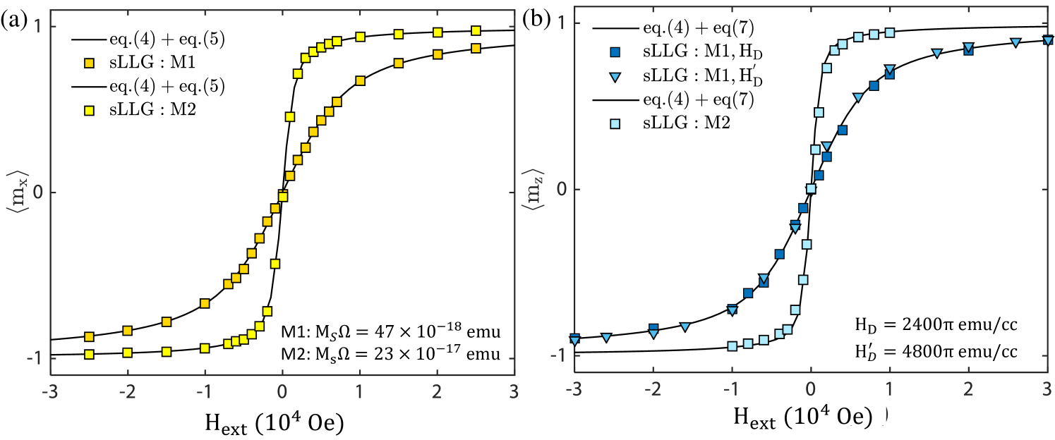
The expression is independent of the demagnetization field. These empirical expressions match our SPICE simulation results quite well as shown in fig. 14.
References
- Yamaoka et al. (2015) M. Yamaoka, C. Yoshimura, M. Hayashi, T. Okuyama, H. Aoki, and H. Mizuno, “24.3 20k-spin ising chip for combinational optimization problem with cmos annealing,” in 2015 IEEE International Solid-State Circuits Conference-(ISSCC), San Francisco, CA, USA (IEEE, 2015) pp. 1–3.
- Neukart et al. (2017) F. Neukart, G. Compostella, C. Seidel, D. Von Dollen, S. Yarkoni, and B. Parney, “Traffic flow optimization using a quantum annealer,” Frontiers in ICT 4, 29 (2017).
- Barahona et al. (1988) F. Barahona, M. Grötschel, M. Jünger, and G. Reinelt, “An application of combinatorial optimization to statistical physics and circuit layout design,” Operations Research 36, 493–513 (1988).
- Cook et al. (2018) C. Cook, H. Zhao, T. Sato, M. Hiromoto, and S. X.-D. Tan, “Gpu based parallel ising computing for combinatorial optimization problems in vlsi physical design,” arXiv preprint arXiv:1807.10750 (2018).
- Rosenberg et al. (2016) G. Rosenberg, P. Haghnegahdar, P. Goddard, P. Carr, K. Wu, and M. L. De Prado, “Solving the optimal trading trajectory problem using a quantum annealer,” IEEE Journal of Selected Topics in Signal Processing 10, 1053–1060 (2016).
- Sakaguchi et al. (2016) H. Sakaguchi, K. Ogata, T. Isomura, S. Utsunomiya, Y. Yamamoto, and K. Aihara, “Boltzmann sampling by degenerate optical parametric oscillator network for structure-based virtual screening,” Entropy 18, 365 (2016).
- Barahona (1982) F. Barahona, “On the computational complexity of ising spin glass models,” Journal of Physics A: Mathematical and General 15, 3241 (1982).
- Lucas (2014) A. Lucas, “Ising formulations of many np problems,” Frontiers in Physics 2, 5 (2014).
- Sutton et al. (2017) B. Sutton, K. Y. Camsari, B. Behin-Aein, and S. Datta, “Intrinsic optimization using stochastic nanomagnets,” Scientific Reports 7, 44370 (2017).
- (10) “Binary stochastic neurons in tensorflow (https://r2rt.com/binary-stochastic-neurons-in-tensorflow.html),” .
- Johnson et al. (2011) M. W. Johnson, M. H. Amin, S. Gildert, T. Lanting, F. Hamze, N. Dickson, R. Harris, A. J. Berkley, J. Johansson, P. Bunyk, et al., “Quantum annealing with manufactured spins,” Nature 473, 194–198 (2011).
- McMahon et al. (2016) P. L. McMahon, A. Marandi, Y. Haribara, R. Hamerly, C. Langrock, S. Tamate, T. Inagaki, H. Takesue, S. Utsunomiya, K. Aihara, et al., “A fully programmable 100-spin coherent ising machine with all-to-all connections,” Science 354, 614–617 (2016).
- Dutta et al. (2020) S. Dutta, A. Khanna, H. Paik, D. Schlom, A. Raychowdhury, Z. Toroczkai, and S. Datta, “Ising hamiltonian solver using stochastic phase-transition nano-oscillators,” arXiv preprint arXiv:2007.12331 (2020).
- Goto, Tatsumura, and Dixon (2019) H. Goto, K. Tatsumura, and A. R. Dixon, “Combinatorial optimization by simulating adiabatic bifurcations in nonlinear hamiltonian systems,” Science advances 5, eaav2372 (2019).
- Wang and Roychowdhury (2019) T. Wang and J. Roychowdhury, “Oim: Oscillator-based ising machines for solving combinatorial optimisation problems,” in International Conference on Unconventional Computation and Natural Computation, Tokyo, Japan (Springer, 2019) pp. 232–256.
- Ahmed, Chiu, and Kim (2020) I. Ahmed, P.-W. Chiu, and C. H. Kim, “A probabilistic self-annealing compute fabric based on 560 hexagonally coupled ring oscillators for solving combinatorial optimization problems,” in 2020 IEEE Symposium on VLSI Circuits, Honolulu, USA (IEEE, 2020) pp. 1–2.
- Chou et al. (2019) J. Chou, S. Bramhavar, S. Ghosh, and W. Herzog, “Analog coupled oscillator based weighted ising machine,” Scientific reports 9, 1–10 (2019).
- Kirkpatrick, Gelatt, and Vecchi (1983) S. Kirkpatrick, C. D. Gelatt, and M. P. Vecchi, “Optimization by simulated annealing,” science 220, 671–680 (1983).
- Baity-Jesi et al. (2014) M. Baity-Jesi, R. A. Baños, A. Cruz, L. A. Fernandez, J. M. Gil-Narvión, A. Gordillo-Guerrero, D. Iñiguez, A. Maiorano, F. Mantovani, E. Marinari, et al., “Janus ii: A new generation application-driven computer for spin-system simulations,” Computer Physics Communications 185, 550–559 (2014).
- Takemoto et al. (2019) T. Takemoto, M. Hayashi, C. Yoshimura, and M. Yamaoka, “2.6 a 2 30k-spin multichip scalable annealing processor based on a processing-in-memory approach for solving large-scale combinatorial optimization problems,” in 2019 IEEE International Solid-State Circuits Conference-(ISSCC), San Francisco, CA, USA (IEEE, 2019) pp. 52–54.
- Aramon et al. (2019) M. Aramon, G. Rosenberg, E. Valiante, T. Miyazawa, H. Tamura, and H. G. Katzgraber, “Physics-inspired optimization for quadratic unconstrained problems using a digital annealer,” Frontiers in Physics 7, 48 (2019).
- Yamamoto et al. (2020) K. Yamamoto, K. Ando, N. Mertig, T. Takemoto, M. Yamaoka, H. Teramoto, A. Sakai, S. Takamaeda-Yamazaki, and M. Motomura, “7.3 statica: A 512-spin 0.25 m-weight full-digital annealing processor with a near-memory all-spin-updates-at-once architecture for combinatorial optimization with complete spin-spin interactions,” in 2020 IEEE International Solid-State Circuits Conference-(ISSCC), San Francisco, CA, USA (IEEE, 2020) pp. 138–140.
- Patel et al. (2020) S. Patel, L. Chen, P. Canoza, and S. Salahuddin, “Ising model optimization problems on a fpga accelerated restricted boltzmann machine,” arXiv preprint arXiv:2008.04436 (2020).
- Patel, Canoza, and Salahuddin (2020) S. Patel, P. Canoza, and S. Salahuddin, “Logically synthesized, hardware-accelerated, restricted boltzmann machines for combinatorial optimization and integer factorization,” arXiv preprint arXiv:2007.13489 (2020).
- Camsari, Salahuddin, and Datta (2017) K. Y. Camsari, S. Salahuddin, and S. Datta, “Implementing p-bits with embedded mtj,” IEEE Electron Device Letters 38, 1767–1770 (2017).
- Xia et al. (2016) L. Xia, P. Gu, B. Li, T. Tang, X. Yin, W. Huangfu, S. Yu, Y. Cao, Y. Wang, and H. Yang, “Technological exploration of rram crossbar array for matrix-vector multiplication,” Journal of Computer Science and Technology 31, 3–19 (2016).
- Cai et al. (2019a) F. Cai, J. M. Correll, S. H. Lee, Y. Lim, V. Bothra, Z. Zhang, M. P. Flynn, and W. D. Lu, “A fully integrated reprogrammable memristor-cmos system for efficient multiply–accumulate operations,” Nature Electronics 2, 290–299 (2019a).
- Bayat et al. (2018) F. M. Bayat, M. Prezioso, B. Chakrabarti, H. Nili, I. Kataeva, and D. Strukov, “Implementation of multilayer perceptron network with highly uniform passive memristive crossbar circuits,” Nature communications 9, 1–7 (2018).
- Sutton et al. (2019) B. Sutton, R. Faria, L. A. Ghantasala, K. Y. Camsari, and S. Datta, “Autonomous probabilistic coprocessing with petaflips per second,” arXiv preprint arXiv:1907.09664 (2019).
- Torunbalci et al. (2018) M. M. Torunbalci, P. Upadhyaya, S. A. Bhave, and K. Y. Camsari, “Modular compact modeling of mtj devices,” IEEE Transactions on Electron Devices 65, 4628–4634 (2018).
- (31) “Predictive Technology Model (PTM) (http://ptm.asu.edu/),” .
- Hassan et al. (2019) O. Hassan, R. Faria, K. Y. Camsari, J. Z. Sun, and S. Datta, “Low-barrier magnet design for efficient hardware binary stochastic neurons,” IEEE Magnetics Letters 10, 1–5 (2019).
- Daniels et al. (2020) M. W. Daniels, A. Madhavan, P. Talatchian, A. Mizrahi, and M. D. Stiles, “Energy-efficient stochastic computing with superparamagnetic tunnel junctions,” Physical Review Applied 13, 034016 (2020).
- Parks et al. (2018) B. Parks, M. Bapna, J. Igbokwe, H. Almasi, W. Wang, and S. A. Majetich, “Superparamagnetic perpendicular magnetic tunnel junctions for true random number generators,” AIP Advances 8, 055903 (2018).
- Grollier et al. (2020) J. Grollier, D. Querlioz, K. Camsari, K. Everschor-Sitte, S. Fukami, and M. D. Stiles, “Neuromorphic spintronics,” Nature Electronics , 1–11 (2020).
- Abeed and Bandyopadhyay (2019) M. A. Abeed and S. Bandyopadhyay, “Low energy barrier nanomagnet design for binary stochastic neurons: Design challenges for real nanomagnets with fabrication defects,” IEEE Magnetics Letters 10, 1–5 (2019).
- Drobitch and Bandyopadhyay (2019) J. L. Drobitch and S. Bandyopadhyay, “Reliability and scalability of p-bits implemented with low energy barrier nanomagnets,” IEEE Magnetics Letters 10, 1–4 (2019).
- Borders et al. (2019) W. A. Borders, A. Z. Pervaiz, S. Fukami, K. Y. Camsari, H. Ohno, and S. Datta, “Integer factorization using stochastic magnetic tunnel junctions,” Nature 573, 390–393 (2019).
- Parks et al. (2020) B. Parks, A. Abdelgawad, T. Wong, R. F. Evans, and S. A. Majetich, “Magnetoresistance dynamics in superparamagnetic co- fe- b nanodots,” Physical Review Applied 13, 014063 (2020).
- Cheemalavagu et al. (2005) S. Cheemalavagu, P. Korkmaz, K. V. Palem, B. E. Akgul, and L. N. Chakrapani, “A probabilistic cmos switch and its realization by exploiting noise,” in IFIP International Conference on VLSI (2005) pp. 535–541.
- Shukla et al. (2014) N. Shukla, A. Parihar, E. Freeman, H. Paik, G. Stone, V. Narayanan, H. Wen, Z. Cai, V. Gopalan, R. Engel-Herbert, et al., “Synchronized charge oscillations in correlated electron systems,” Scientific reports 4, 4964 (2014).
- Kumar, Strachan, and Williams (2017) S. Kumar, J. P. Strachan, and R. S. Williams, “Chaotic dynamics in nanoscale nbo 2 mott memristors for analogue computing,” Nature 548, 318–321 (2017).
- Stampfer et al. (2018) B. Stampfer, F. Zhang, Y. Y. Illarionov, T. Knobloch, P. Wu, M. Waltl, A. Grill, J. Appenzeller, and T. Grasser, “Characterization of single defects in ultrascaled mos 2 field-effect transistors,” ACS nano 12, 5368–5375 (2018).
- Cai et al. (2019b) J. Cai, B. Fang, L. Zhang, W. Lv, B. Zhang, T. Zhou, G. Finocchio, and Z. Zeng, “Voltage-controlled spintronic stochastic neuron based on a magnetic tunnel junction,” Physical Review Applied 11, 034015 (2019b).
- Camsari et al. (2020) K. Y. Camsari, M. M. Torunbalci, W. A. Borders, H. Ohno, and S. Fukami, “Double free-layer magnetic tunnel junctions for probabilistic bits,” arXiv preprint arXiv:2012.06950 (2020).
- Lin et al. (2009) C. Lin, S. Kang, Y. Wang, K. Lee, X. Zhu, W. Chen, X. Li, W. Hsu, Y. Kao, M. Liu, et al., “45nm low power cmos logic compatible embedded stt mram utilizing a reverse-connection 1t/1mtj cell,” in 2009 IEEE International Electron Devices Meeting (IEDM), San Francisco, CA, USA (IEEE, 2009) pp. 1–4.
- Camsari et al. (2017) K. Y. Camsari, R. Faria, B. M. Sutton, and S. Datta, “Stochastic p-bits for invertible logic,” Physical Review X 7, 031014 (2017).
- Lv, Bloom, and Wang (2019) Y. Lv, R. P. Bloom, and J.-P. Wang, “Experimental demonstration of probabilistic spin logic by magnetic tunnel junctions,” IEEE Magnetics Letters 10, 1–5 (2019).
- Zink, Lv, and Wang (2019) B. R. Zink, Y. Lv, and J.-P. Wang, “Independent control of antiparallel-and parallel-state thermal stability factors in magnetic tunnel junctions for telegraphic signals with two degrees of tunability,” IEEE Transactions on Electron Devices 66, 5353–5359 (2019).
- Parkin et al. (2004) S. S. Parkin, C. Kaiser, A. Panchula, P. M. Rice, B. Hughes, M. Samant, and S.-H. Yang, “Giant tunnelling magnetoresistance at room temperature with mgo (100) tunnel barriers,” Nature materials 3, 862–867 (2004).
- Ikeda et al. (2008) S. Ikeda, J. Hayakawa, Y. Ashizawa, Y. Lee, K. Miura, H. Hasegawa, M. Tsunoda, F. Matsukura, and H. Ohno, “Tunnel magnetoresistance of 604% at 300 k by suppression of ta diffusion in co fe b/ mg o/ co fe b pseudo-spin-valves annealed at high temperature,” Applied Physics Letters 93, 082508 (2008).
- Debashis et al. (2018) P. Debashis, R. Faria, K. Y. Camsari, and Z. Chen, “Design of stochastic nanomagnets for probabilistic spin logic,” IEEE Magnetics Letters 9, 1–5 (2018).
- Debashis et al. (2016) P. Debashis, R. Faria, K. Y. Camsari, J. Appenzeller, S. Datta, and Z. Chen, “Experimental demonstration of nanomagnet networks as hardware for ising computing,” in 2016 IEEE International Electron Devices Meeting (IEDM), San Francisco, CA, USA (IEEE, 2016) pp. 34–3.
- Safranski et al. (2020) C. Safranski, J. Kaiser, P. Trouilloud, P. Hashemi, G. Hu, and J. Z. Sun, “Demonstration of nanosecond operation in stochastic magnetic tunnel junctions,” arXiv preprint arXiv:2010.14393 (2020).
- Zhang et al. (2021) C. Zhang, Y. Takeuchi, S. Fukami, and H. Ohno, “Field-free and sub-ns magnetization switching of magnetic tunnel junctions by combining spin-transfer torque and spin–orbit torque,” Applied Physics Letters 118, 092406 (2021).
- (56) nanohub.org, “Modular approach to spintronics,” https://nanohub.org/groups/spintronics.
- Coffey and Kalmykov (2012) W. T. Coffey and Y. P. Kalmykov, “Thermal fluctuations of magnetic nanoparticles: Fifty years after brown,” Journal of Applied Physics 112, 121301 (2012).
- Kaiser et al. (2019) J. Kaiser, A. Rustagi, K. Y. Camsari, J. Z. Sun, S. Datta, and P. Upadhyaya, “Subnanosecond fluctuations in low-barrier nanomagnets,” Physical Review Applied 12, 054056 (2019).
- Pufall et al. (2004) M. R. Pufall, W. H. Rippard, S. Kaka, S. E. Russek, T. J. Silva, J. Katine, and M. Carey, “Large-angle, gigahertz-rate random telegraph switching induced by spin-momentum transfer,” Physical Review B 69, 214409 (2004).
- Faria, Camsari, and Datta (2017) R. Faria, K. Y. Camsari, and S. Datta, “Low-barrier nanomagnets as p-bits for spin logic,” IEEE Magnetics Letters 8, 1–5 (2017).
- Sun (2000) J. Z. Sun, “Spin-current interaction with a monodomain magnetic body: A model study,” Physical Review B 62, 570 (2000).
- Faria, Camsari, and Datta (2018) R. Faria, K. Y. Camsari, and S. Datta, “Implementing bayesian networks with embedded stochastic mram,” AIP Advances 8, 045101 (2018).
- Romera et al. (2018) M. Romera, P. Talatchian, S. Tsunegi, F. A. Araujo, V. Cros, P. Bortolotti, J. Trastoy, K. Yakushiji, A. Fukushima, H. Kubota, et al., “Vowel recognition with four coupled spin-torque nano-oscillators,” Nature 563, 230–234 (2018).
- Jenkins et al. (2019) S. Jenkins, A. Meo, L. E. Elliott, S. K. Piotrowski, M. Bapna, R. W. Chantrell, S. A. Majetich, and R. F. Evans, “Magnetic stray fields in nanoscale magnetic tunnel junctions,” Journal of Physics D: Applied Physics 53, 044001 (2019).
- Faria et al. (2020) R. Faria, J. Kaiser, K. Y. Camsari, and S. Datta, “Hardware design for autonomous bayesian networks,” arXiv preprint arXiv:2003.01767 (2020).
- Isakov et al. (2015) S. V. Isakov, I. N. Zintchenko, T. F. Rønnow, and M. Troyer, “Optimised simulated annealing for ising spin glasses,” Computer Physics Communications 192, 265–271 (2015).
- Aarts, Aarts, and Lenstra (2003) E. Aarts, E. H. Aarts, and J. K. Lenstra, Local search in combinatorial optimization (Princeton University Press, NJ, USA, 2003).
- Kaiser et al. (2020) J. Kaiser, R. Faria, K. Y. Camsari, and S. Datta, “Probabilistic circuits for autonomous learning: A simulation study,” Frontiers in Computational Neuroscience 14, 14:1–7 (2020).
- Cai et al. (2019c) F. Cai, S. Kumar, T. Van Vaerenbergh, R. Liu, C. Li, S. Yu, Q. Xia, J. J. Yang, R. Beausoleil, W. Lu, et al., “Harnessing intrinsic noise in memristor hopfield neural networks for combinatorial optimization,” arXiv preprint arXiv:1903.11194 (2019c).
- Huang et al. (2015) H. Huang, J. Heilmeyer, M. Grözing, M. Berroth, J. Leibrich, and W. Rosenkranz, “An 8-bit 100-gs/s distributed dac in 28-nm cmos for optical communications,” IEEE Transactions on Microwave Theory and Techniques 63, 1211–1218 (2015).
- Hu et al. (2018) M. Hu, C. E. Graves, C. Li, Y. Li, N. Ge, E. Montgomery, N. Davila, H. Jiang, R. S. Williams, J. J. Yang, et al., “Memristor-based analog computation and neural network classification with a dot product engine,” Advanced Materials 30, 1705914 (2018).
- Gyoten, Hiromoto, and Sato (2018) H. Gyoten, M. Hiromoto, and T. Sato, “Area efficient annealing processor for ising model without random number generator,” IEICE TRANSACTIONS on Information and Systems 101, 314–323 (2018).
- Aggarwal et al. (2019) S. Aggarwal, H. Almasi, M. DeHerrera, B. Hughes, S. Ikegawa, J. Janesky, H. Lee, H. Lu, F. Mancoff, K. Nagel, et al., “Demonstration of a reliable 1 gb standalone spin-transfer torque mram for industrial applications,” in 2019 IEEE International Electron Devices Meeting (IEDM), San Francisco, CA, USA (IEEE, 2019) pp. 2–1.
- eve (2019) “Everspin enters pilot production phase for the world’s first 28 nm 1 gb stt-mram component,” Everspin Technology (2019).
- Zhang et al. (2020) X. Zhang, R. Bashizade, Y. Wang, C. Lyu, S. Mukherjee, and A. R. Lebeck, “Beyond application end-point results: Quantifying statistical robustness of mcmc accelerators,” arXiv preprint arXiv:2003.04223 (2020).
- Nasrin et al. (2019) S. Nasrin, J. L. Drobitch, S. Bandyopadhyay, and A. R. Trivedi, “Low power restricted boltzmann machine using mixed-mode magneto-tunneling junctions,” IEEE Electron Device Letters 40, 345–348 (2019).
- Schuman et al. (2017) C. D. Schuman, T. E. Potok, R. M. Patton, J. D. Birdwell, M. E. Dean, G. S. Rose, and J. S. Plank, “A survey of neuromorphic computing and neural networks in hardware,” arXiv preprint arXiv:1705.06963 (2017).
- Hinton (2002) G. E. Hinton, “Training products of experts by minimizing contrastive divergence,” Neural computation 14, 1771–1800 (2002).
- Courbariaux et al. (2016) M. Courbariaux, I. Hubara, D. Soudry, R. El-Yaniv, and Y. Bengio, “Binarized neural networks: Training neural networks with weights and activations constrained to+ 1 or-1,” arXiv preprint arXiv:1602.02830 2 (2016).
- Tsai et al. (2017) C.-H. Tsai, W.-J. Yu, W. H. Wong, and C.-Y. Lee, “A 41.3/26.7 pj per neuron weight rbm processor supporting on-chip learning/inference for iot applications,” IEEE Journal of Solid-State Circuits 52, 2601–2612 (2017).
- Park et al. (2015) S. Park, K. Bong, D. Shin, J. Lee, S. Choi, and H.-J. Yoo, “93tops/w scalable deep learning/inference processor with tetra-parallel mimd architecture for big-data applications,” in 2015 IEEE International Solid-State Circuits Conference-(ISSCC), San Francisco, CA, USA (IEEE, 2015) pp. 1–3.
- Brown Jr (1963) W. F. Brown Jr, “Thermal fluctuations of a single-domain particle,” Physical Review 130, 1677 (1963).
- Sayed et al. (2019) S. Sayed, K. Y. Camsari, R. Faria, and S. Datta, “Rectification in spin-orbit materials using low-energy-barrier magnets,” Physical Review Applied 11, 054063 (2019).