This paper was converted on www.awesomepapers.org from LaTeX by an anonymous user.
Want to know more? Visit the Converter page.

footnotetext: z School of Mathematics, Jilin University, Changchun 130012, P. R. China. tongzc20@mails.jlu.edu.cn x The corresponding author. School of Mathematics, Jilin University, Changchun 130012, P. R. China; Center for Mathematics and Interdisciplinary Sciences, Northeast Normal University, Changchun 130024, P. R. China. liyong@jlu.edu.cn

Quantitative uniform exponential acceleration of averages along decaying waves

Zhicheng Tong z, Yong Li x
Abstract

In this study, utilizing a specific exponential weighting function, we investigate the uniform exponential convergence of weighted Birkhoff averages along decaying waves and delve into several related variants. A key distinction from traditional scenarios is evident here: despite reduced regularity in observables, our method still maintains exponential convergence. In particular, we develop new techniques that yield very precise rates of exponential convergence, as evidenced by numerical simulations. Furthermore, this innovative approach extends to quantitative analyses involving different weighting functions employed by others, surpassing the limitations inherent in prior research. It also enhances the exponential convergence rates of weighted Birkhoff averages along quasi-periodic orbits via analytic observables. To the best of our knowledge, this is the first result on the uniform exponential acceleration beyond averages along quasi-periodic or almost periodic orbits, particularly from a quantitative perspective.

Keywords: Weighted averaging method, decaying waves, quantitative uniform exponential convergence, numerical simulation
2020 Mathematics Subject Classification: 37A25, 37A30, 37A46

1 Introduction

As one of the foundational theories in dynamical systems, ergodic theory first originated from Birkhoff and von Neumann. This seminal work has given rise to an array of diverse formulations and has been extensively applied across various domains. It is a well-established fact, as noted by Krengel [16], that the convergence rates of Birkhoff averages in ergodic theory are generally slow, and can even be arbitrarily slow for certain counterexamples. Similar assertions were reaffirmed by Ryzhikov [36], while recent results on the convergence rate within the Birkhoff ergodic theorem can be found in Podvigin’s comprehensive survey [24]. Furthermore, Yoccoz’s counterexamples [39, 40], constructed via rotations that are extremely Liouvillean–nearly rational–on the finite-dimensional torus, deserve mentioning. Such slow convergence is ubiquitous in ergodic theory and is intrinsically inescapable, and it would be at most 𝒪(N1)\mathcal{O}(N^{-1}) in non-trivial cases with time length NN, i.e., the observables are non-constant, as detailed by Kachurovskiĭ [13]. More frustratingly, the pursuit of high-precision numerical results may demand computational durations on the order of billions of years, a point elaborated by Das and Yorke in [5].

Given the acknowledged slow convergence in ergodic theory, the weighting method is crucial for accelerating computations in both mathematics and mechanics. There is a growing interest in identifying suitable weighting functions to enhance the convergence rates of ergodic averages. To investigate quasi-periodic perturbations of quasi-periodic flows, Laskar employed a weighting function sin2(πx)\sin^{2}(\pi x) to accelerate computational processes, as detailed in [17, 18, 19]. Furthermore, Laskar claimed that a specific exponential weighting function possesses superior asymptotic characteristics, although he did not implement it or provide evidence of its convergence properties, as noted in [19]. It is worth highlighting that the resulting convergence rate can be demonstrated to exceed that of any arbitrary polynomial, which we shall detail later. To be more precise, Laskar employed the following weighting function to investigate ergodicity within dynamical systems:

w(x):={(01exp(s1(1s)1)𝑑s)1exp(x1(1x)1),x(0,1),0,x(0,1),{w}\left(x\right):=\left\{\begin{array}[]{ll}{\left({\int_{0}^{1}{\exp\left({-{s^{-1}}{{\left({1-s}\right)}^{-1}}}\right)ds}}\right)^{-1}}\exp\left({-{x^{-1}}{{\left({1-x}\right)}^{-1}}}\right),&x\in\left({0,1}\right),\hfill\\ 0,&x\notin\left(0,1\right),\hfill\\ \end{array}\right. (1.1)

and the corresponding weighted Birkhoff average of an sufficiently smooth observable ff evaluated along a trajectory of length NN reads

WBN(f)(x):=1ANn=0N1w(n/N)f(Tnx),{\rm{WB}}_{N}\left(f\right)\left(x\right):=\frac{1}{{{A_{N}}}}\sum\limits_{n=0}^{N-1}{w\left({n/N}\right)f\left({{T^{n}}x}\right)}, (1.2)

provided AN:=n=0N1w(n/N){A_{N}}:=\sum\nolimits_{n=0}^{N-1}{w\left({n/N}\right)}, and TT is a quasi-periodic mapping on the dd-torus 𝕋d\mathbb{T}^{d} with d+d\in\mathbb{N}^{+}, x𝕋dx\in\mathbb{T}^{d} is an initial point. It is evident that wC0([0,1])w\in C_{0}^{\infty}\left({\left[{0,1}\right]}\right) and the integral 01w(x)𝑑x=1\int_{0}^{1}{w\left(x\right)dx}=1. From a statistical standpoint, this approach effectively reduces the impact of the initial and terminal data, thereby highlighting those in the central range. This emphasis aligns with the concept of averaging, consequently leading to an intuitively rapid uniform convergence to the spatial average 𝕋df(θ)𝑑θ\int_{{\mathbb{T}^{d}}}{f\left(\theta\right)d\theta}. However, there are more profound reasons behind this phenomenon, which have been illustrated by the authors in [34].

Back to the main topic, following Laskar’s significant numerical discovery, Das and Yorke [5] provided rigorous proofs for quasi-periodic systems with Diophantine rotations. To be more precise, they demonstrated that under CC^{\infty} observables, the weighted Birkhoff averages can achieve rapid convergence of arbitrary polynomial order. However, more rigorous theoretical work is still lacking in this area. To this end, inspired by the fundamental work of Das and Yorke, the authors recently made interesting findings in [34, 35, 33]–namely that universally–or saying in terms of full measure, the weighted Birkhoff averages (as well as the Cesàro weighted averages) exhibit exponential convergence as long as the observables are analytic and irrespective of finite dimensions (quasi-periodic) or infinite dimensions (almost periodic). This comes somewhat unexpectedly since it can break through what is known as “curse of dimensionality”–a common phenomenon in high-dimensional systems where complexity grows exponentially with each additional dimension. More generally, the authors also discussed abstract scenarios admitting weaker nonresonance and regularity and present certain balancing criteria to achieve rapid convergence. Due to brevity considerations, these details are not elaborated upon here.

Based on these theoretical foundations, many researchers have utilized this weighting method to perform numerical calculations on various physical systems which has significantly increased their efficiency. On this aspect, see Calleja et al. [4], Das et al. [6], Sander and Meiss [27, 28, 29], Meiss and Sander [22], Duignan and Meiss [9], Blessing and Mireles James [3] among several others; these contributions provide strong evidence supporting rapid convergence. Specifically, Duignan and Meiss [9] employed this weighting method to distinguish between regular (in fact, quasi-periodic there) and chaotic systems. To be more precise, under the weighted Birkhoff averages via (1.1), regular systems typically demonstrate a rapid exponential convergence. In contrast, chaotic systems exhibit at most an one-order polynomial slow convergence. This raises an intriguing question: what other scenarios might these so-called regular systems applicable to weighted Birkhoff averages encompass?

The primary motivations behind this work are twofold: (M1) We aim to delve deeper into the practical applications of weighted Birkhoff averages beyond quasi-periodic and almost periodic systems which admit zero Lyapunov exponents. We believe at least that, for dynamical systems having negative maximal Lyapunov exponents, Birkhoff averages along trajectories, once weighted by the function (1.1), should also exhibit exponential convergence under certain generic conditions. (M2) Currently, the analysis of the convergence rates for the weighted Birkhoff averages with the weighting function (1.1) is almost entirely qualitative (at least, not particularly precise when compared with numerical simulations of the convergence rates). We suspect that this imprecision is due to limitations in previous techniques. Therefore, we aim to develop new approaches to provide a quantitative version of these convergence rates.

Based on the above considerations, we first start with some typical examples, namely exponentially decaying waves (e.g., eλxsin(ρx)e^{-\lambda x}\sin(\rho x) and eλxcos(ρx)e^{-\lambda x}\cos(\rho x) with certain λ>0\lambda>0 and ρ\rho\in\mathbb{R}), which constitute some fundamental solutions among others for linear matrix differential equations described as x=Axx^{\prime}=Ax (other solutions have more polynomial parts than these, depending on the multiplicity of the eigenvalues, see Section 6), where all eigenvalues of the constant matrix AA lie inside the unit circle 𝕊1\mathbb{S}^{1}. Such decaying waves can also be interpreted as projections onto planes from spiral waves within 33-dimensional space. For further insights into the connections between decaying waves and dynamics systems, we refer readers to Liu et al. [20, 21], Wang et al. [37], Xing et al. [38] inclusive of their references which provide an exploration into this domain. As a main contribution, we demonstrate that Laskar’s weighted averaging method not only significantly accelerates the Birkhoff averages along quasi-periodic or almost periodic orbits, but also proves effective for other scenarios, involving weighted Birkhoff averages of decaying waves, with extremely rapid exponential convergence rates contrasting with the universal one-order polynomial type observed in unweighted cases (Theorem 1.1 and Remark 1.1). Specifically, our quantitative convergence rates prove to be remarkably precise, as evidenced by the numerical simulations illustrated in Figure 1 within Section 8. Furthermore, we proceed to discuss more general decaying waves in series forms and arrive at optimal results somewhat unexpectedly (Theorem 1.2).

Before delving into the main subject, let us first introduce some basic notations for the sake of simplicity. We define that in the limit process as x+x\to+\infty, the statements f1(x)=𝒪(f2(x))f_{1}(x)=\mathcal{O}\left(f_{2}(x)\right) and f1(x)=𝒪#(f2(x))f_{1}(x)=\mathcal{O}^{\#}\left(f_{2}(x)\right) imply there exists a positive constant c>0c>0, such that |f1(x)|cf2(x)|f_{1}(x)|\leqslant cf_{2}(x) and c1f2(x)|f1(x)|cf2(x)c^{-1}f_{2}(x)\leqslant|f_{1}(x)|\leqslant cf_{2}(x), respectively. We also denote by DnfD^{n}f the nn-th derivative of a sufficiently smooth function ff. Additionally, for any fixed number xx\in\mathbb{R}, we define x𝕋:=infn|x2πn|{\left\|x\right\|_{\mathbb{T}}}:={\inf_{n\in\mathbb{Z}}}\left|{x-2\pi n}\right| as the distance to the closest element of the set 2π2\pi\mathbb{Z}, or equivalently, it represents the metric on the standard torus 𝕋:=/2π\mathbb{T}:=\mathbb{R}/2\pi\mathbb{Z} identified with [0,2π)[0,2\pi).

In what follows, we proceed to present our main results. Consider the unweighted time average of the decaying wave as

DWN(λ,ρ,θ):=1Nn=0N1eλnsin(θ+nρ),{{\rm{DW}}_{N}}\left({\lambda,\rho,\theta}\right):=\frac{1}{N}\sum\limits_{n=0}^{N-1}{{e^{-\lambda n}}\sin\left({\theta+n\rho}\right)},

as well as the ww-weighted type given by

WDWN(λ,ρ,θ):=1ANn=0N1w(n/N)eλnsin(θ+nρ).{\rm{WDW}}_{N}\left({\lambda,\rho,\theta}\right):=\frac{1}{{{A_{N}}}}\sum\limits_{n=0}^{N-1}{w\left({n/N}\right){e^{-\lambda n}}\sin\left({\theta+n\rho}\right)}.

The first main result in this paper is stated as follows.

Theorem 1.1.

(I) For any fixed λ>0\lambda>0 and ρ\rho\in\mathbb{R},

|WDWN(λ,ρ,θ)|=𝒪(exp(ξN)),N+\left|{{\rm{WDW}}_{N}\left({\lambda,\rho,\theta}\right)}\right|=\mathcal{O}\left({\exp\left({-{\xi}\sqrt{N}}\right)}\right),\;\;N\to+\infty

uniformly holds with θ\theta\in\mathbb{R}, where ξ=ξ(λ,ρ)=2λ+e1λ2+ρ𝕋2>0\xi=\xi(\lambda,\rho)=\sqrt{2\lambda}+{e^{-1}}\sqrt{{\lambda^{2}}+\left\|\rho\right\|_{\mathbb{T}}^{2}}>0. In particular, the control coefficient is independent of ρ\rho, and is uniformly bounded for large λ\lambda.
(II) However, for any fixed λ>0\lambda>0 and ρ,θ\rho,\theta\in\mathbb{R}, there exists infinitely many N+N\in\mathbb{N}^{+} such that

|DWN(λ,ρ,θ)|=𝒪#(N1),N+,\left|{{{\rm{DW}}_{N}}\left({\lambda,\rho,\theta}\right)}\right|={\mathcal{O}^{\#}}\left({{N^{-1}}}\right),\;\;N\to+\infty,

whenever eλsin(ρθ)+sinθ0{e^{-\lambda}}\sin\left({\rho-\theta}\right)+\sin\theta\neq 0.

Remark 1.1.

For fixed λ>0\lambda>0 and ρ\rho\in\mathbb{R}, the set of such θ\theta\in\mathbb{R} has at most zero Lebesgue measure. Therefore, the 𝒪(N1)\mathcal{O}\left(N^{-1}\right) convergence for the unweighted decaying waves is universal, or commonly referred to as almost certain. This is completely consistent with the zero-one law in [24].

Theorem 1.1 provides an upper bound on the convergence rate of the weighted Birkhoff average WDWN(λ,ρ,θ){{\rm{WDW}}_{N}\left({\lambda,\rho,\theta}\right)}, which depends simultaneously on the decaying parameter λ\lambda and the rotating parameter ρ\rho. As we will demonstrate in the numerical simulation within Section 8, this estimate is remarkably precise.

The following conclusion concerning the averages of superimposed waves is a direct corollary of Theorem 1.1.

Corollary 1.1.

For kk\in\mathbb{N}, define gk(x,θ):=eλkxsin(θ+xρk){g_{k}}\left({x,\theta}\right):={e^{-{\lambda_{k}}x}}\sin\left({\theta+x{\rho_{k}}}\right), where infkλk>0\mathop{\inf}\nolimits_{k\in\mathbb{N}}{\lambda_{k}}>0 and ρk,θ{\rho_{k}},\theta\in\mathbb{R}. Then for any sequence {ck}kl1{\left\{{{c_{k}}}\right\}_{k\in\mathbb{N}}}\in{l^{1}}, the time average 1ANn=0N1w(n/N)g(n,θ)\frac{1}{A_{N}}\sum\nolimits_{n=0}^{N-1}{w(n/N)g\left({n,\theta}\right)} of the superimposed wave g(x,θ)=kckgk(x,θ)g\left({x,\theta}\right)=\sum\nolimits_{k\in\mathbb{N}}{{c_{k}}{g_{k}}\left({x,\theta}\right)} converges uniformly (with respect to θ\theta) and exponentially to 0.

Indeed, when the decaying parameters λk=λ>0\lambda_{k}=\lambda>0, Corollary 1.1 covers the cases of decaying quasi-periodic or decaying almost periodic. For a given set of rotation parameters {ρk}k=1d\{\rho_{k}\}_{k=1}^{d} with 1d<+1\leqslant d<+\infty (=+=+\infty), if for any 0kd0\neq k\in\mathbb{Z}^{d}, j=1dkjρj0\sum\nolimits_{j=1}^{d}{k_{j}\rho_{j}}\neq 0, then the motion exhibited is quasi-periodic (almost periodic). See [33] for further characterization of these two concepts, as well as specific examples in Kozlov [15], for instance. However, the control coefficient in Theorem 1.1 may tend to ++\infty as the decaying parameter λ\lambda tends to 0+0^{+}. Therefore, if the case considered in Corollary 1.1 allows the decaying parameters λk\lambda_{k} to tend to 0+0^{+} (acting similarly to Bessel functions), then with the variation in the arithmetic properties of the rotation parameters ρk\rho_{k}, more complicated small denominator problems may arise. This needs to be dealt with in combination with the techniques in [33, 34, 35] (see also Section 7), which we prefer not to discuss here.

To enhance the applicability of our results, we present the quantitative Theorem 1.2 below. Prior to this, we denote by A(𝕋)A(\mathbb{T}) the space consisting of continuous functions on 𝕋\mathbb{T} having an absolutely convergent Fourier series, i.e., the functions f(x)=kf^keikxf\left(x\right)=\sum\nolimits_{k\in\mathbb{Z}}{{{\hat{f}}_{k}}{e^{ikx}}} for which k|f^k|<+\sum\nolimits_{k\in\mathbb{Z}}{|{{\hat{f}}_{k}}|}<+\infty. With the norm defined by fA(𝕋):=k|f^k|{\left\|f\right\|_{A\left(\mathbb{T}\right)}}:=\sum\nolimits_{k\in\mathbb{Z}}{|{{\hat{f}}_{k}}|}, A(𝕋){A\left(\mathbb{T}\right)} is a Banach space isometric to l1l^{1} with algebra property, see Katznelson [14] for instance. For 0<α<10<\alpha<1, we denote by Cα(𝕋)C^{\alpha}(\mathbb{T}) the space of α\alpha-Hölder functions endowed with the norm

fCα(𝕋):=supx𝕋|f(x)|+supx,y𝕋,xy|f(x)f(y)||xy|α<+.{\left\|f\right\|_{{C^{\alpha}}\left(\mathbb{T}\right)}}:=\mathop{\sup}\limits_{x\in\mathbb{T}}\left|{f\left(x\right)}\right|+\mathop{\sup}\limits_{x,y\in\mathbb{T},\;x\neq y}\frac{{\left|{f\left(x\right)-f\left(y\right)}\right|}}{{{{\left|{x-y}\right|}^{\alpha}}}}<+\infty.

We also denote by Cn(𝕋)C^{n}(\mathbb{T}) the space of functions on 𝕋\mathbb{T} with nn-order continuous derivatives, where nn\in\mathbb{N}.

Theorem 1.2.

Let λ>0\lambda>0, ρ,θ\rho,\theta\in\mathbb{R} be given.

  • (I)

    For any observable 𝒫(x)A(𝕋)\mathscr{P}(x)\in A(\mathbb{T}), it holds uniformly with respect to θ\theta that

    |1ANn=0N1w(n/N)eλn𝒫(θ+nρ)|=𝒪(exp(ξN)),N+,\left|{\frac{1}{{{A_{N}}}}\sum\limits_{n=0}^{N-1}{w\left({n/N}\right){e^{-\lambda n}}\mathscr{P}\left({\theta+n\rho}\right)}}\right|=\mathcal{O}\left({\exp\left({-\xi^{\prime}\sqrt{N}}\right)}\right),\;\;N\to+\infty, (1.3)

    where ξ=ξ(λ,0)=2λ+e1λ>0\xi^{\prime}=\xi(\lambda,0)=\sqrt{2\lambda}+{e^{-1}}\lambda>0. A sufficient case is 𝒫(x)Cα(𝕋){\mathscr{P}}(x)\in C^{\alpha}(\mathbb{T}) with α>1/2\alpha>1/2. In particular, for any trigonometric polynomial of order \ell on 𝕋\mathbb{T} without the Fourier constant term, i.e., 𝒫(x)=n=1(ancosnx+bnsinnx)\mathscr{P}\left(x\right)=\sum\nolimits_{n=1}^{\ell}{\left({{a_{n}}\cos nx+{b_{n}}\sin nx}\right)}, the index ξ\xi^{\prime} of the exponential rate in (1.3) could be improved to ξ=2λ+e1λ2+min1jjρ𝕋2{\xi^{*}}=\sqrt{2\lambda}+{e^{-1}}\sqrt{{\lambda^{2}}+\mathop{\min}\nolimits_{1\leqslant j\leqslant\ell}\left\|{j\rho}\right\|_{\mathbb{T}}^{2}}.

  • (II)

    For any analytic observable 𝒬(x)\mathscr{Q}(x) on [1,1][-1,1], it holds uniformly with respect to θ\theta that

    |1ANn=0N1w(n/N)𝒬(eλnsin(θ+nρ))𝒬(0)|=𝒪(exp(ξN)),N+,\left|{\frac{1}{{{A_{N}}}}\sum\limits_{n=0}^{N-1}{w\left({n/N}\right)\mathscr{Q}\left({{e^{-\lambda n}}\sin\left({\theta+n\rho}\right)}\right)}-\mathscr{Q}\left(0\right)}\right|=\mathcal{O}\left({\exp\left({-\xi^{\prime}\sqrt{N}}\right)}\right),\;\;N\to+\infty, (1.4)

    where ξ=ξ(λ,0)=2λ+e1λ>0\xi^{\prime}=\xi(\lambda,0)=\sqrt{2\lambda}+{e^{-1}}\lambda>0. In particular, for any polynomial of order ν\nu, i.e., 𝒬(x)=j=0ν𝒬jxj\mathscr{Q}\left(x\right)=\sum\nolimits_{j=0}^{\nu}{{\mathscr{Q}_{j}}{x^{j}}}, the index ξ\xi^{\prime} of the exponential rate in (1.4) could be improved to ξ=min{ξ(1),ξ(2)}{\xi_{*}}=\min\{{\xi_{*}^{(1)},\xi_{*}^{(2)}}\}, provided

    ξ(1)=min{ξ(jλ,0)=2jλ+e1jλ:for even j with 0jν and 𝒬j0}\xi_{*}^{(1)}=\min\left\{{\xi\left({j\lambda,0}\right)=\sqrt{2j\lambda}+{e^{-1}}j\lambda:\;\text{for even $j$ with $0\leqslant j\leqslant\nu$ and ${\mathscr{Q}_{j}}\neq 0$}}\right\}

    and

    ξ(2)=min{ξ(jλ,jρ)=2jλ+e1j2λ2+jρ𝕋2:for odd j with 0jν and 𝒬j0}.\xi_{*}^{(2)}=\min\left\{{\xi\left({j\lambda,j\rho}\right)=\sqrt{2j\lambda}+{e^{-1}}\sqrt{{j^{2}}{\lambda^{2}}+\left\|{j\rho}\right\|_{\mathbb{T}}^{2}}:\;\text{for odd $j$ with $0\leqslant j\leqslant\nu$ and ${\mathscr{Q}_{j}}\neq 0$}}\right\}.
  • (III)

    For any observable 𝒦(x)\mathscr{K}(x) on [1,1][-1,1] with |𝒦(x)𝒦(0)|Mx2τ\left|{\mathscr{K}\left(x\right)-\mathscr{K}\left(0\right)}\right|\leqslant M{x^{2\tau}} for some M>0M>0 and τ+\tau\in\mathbb{N}^{+}, it holds uniformly with respect to θ\theta that

    |1ANn=0N1w(n/N)𝒦(eλnsin(θ+nρ))𝒦(0)|=𝒪(exp(ξN)),N+,\left|{\frac{1}{{{A_{N}}}}\sum\limits_{n=0}^{N-1}{w\left({n/N}\right)\mathscr{K}\left({{e^{-\lambda n}}\sin\left({\theta+n\rho}\right)}\right)}-\mathscr{K}\left(0\right)}\right|=\mathcal{O}\left({\exp\left({-\xi_{*}^{*}\sqrt{N}}\right)}\right),\;\;N\to+\infty,

    where ξ=ξ(2τλ,0)=2τλ+2e1τλ>0{\xi_{*}^{*}}=\xi\left({2\tau\lambda,0}\right)=2\sqrt{\tau\lambda}+2{e^{-1}}\tau\lambda>0. A sufficient case is 𝒦(x)C2τ(𝕋)\mathscr{K}(x)\in{C^{2\tau}}\left(\mathbb{T}\right) satisfying Dj𝒦(0)=0{D^{j}}\mathscr{K}\left(0\right)=0 for 1j2τ11\leqslant j\leqslant 2\tau-1 and D2τ𝒦(0)0{D^{2\tau}}\mathscr{K}\left(0\right)\neq 0.

Remark 1.2.

The sufficient case 𝒫(x)Cα(𝕋){\mathscr{P}}(x)\in C^{\alpha}(\mathbb{T}) with α>1/2\alpha>1/2 is indeed optimal for 𝒫(x)A(𝕋)\mathscr{P}(x)\in A(\mathbb{T}) in (I), namely there exists a counterexample (Hardy-Littlewood series) f~(x)C1/2(𝕋)\tilde{f}(x)\in C^{1/2}(\mathbb{T}) such that f~(x)A(𝕋)\tilde{f}(x)\notin A(\mathbb{T}), see Zygmund [43] and Katznelson [14] for instance.

Remark 1.3.

For trigonometric series, the absolute summability in (I) is almost optimal in order to guarantee the uniform convergence with respect to θ\theta in (1.3). For example, considering an>0a_{n}>0 and nan=+\sum\nolimits_{n\in\mathbb{Z}}{{a_{n}}}=+\infty, we construct the counterexample as f¯(x)=nancosnx\bar{f}\left(x\right)=\sum\nolimits_{n\in\mathbb{Z}}{{a_{n}}\cos nx}. Then f¯(0)=+\bar{f}\left(0\right)=+\infty. Taking ρ=0\rho=0 and θ>0\theta>0 sufficiently close to 0, the weighed decaying wave becomes (1ANn=0N1w(n/N)eλn)f¯(θ)\left({\frac{1}{{{A_{N}}}}\sum\nolimits_{n=0}^{N-1}{w\left({n/N}\right){e^{-\lambda n}}}}\right)\bar{f}\left(\theta\right), which exhibits non-uniform convergence for such θ\theta.

Recall that in [22, 5, 33], achieving fast convergence of the weighted Birkhoff average necessitates strong regularity for the observable, e.g., the CC^{\infty} regularity or even analyticity. However, as shown for the decaying wave in (I), incorporating the decaying part compensates for the lack of regularity, thereby naturally achieving the exponential convergence. Moreover, the observable in (III) could admit very weak regularity, for example, discontinuity except of x=0x=0.

The remainder of this paper is organized as follows. To highlight the ideas underlying our proof, we provide a detailed analysis of Theorem 1.1 in Section 2. Building upon this foundation, we give a more concise proof for Theorem 1.2 in Section 4. We also quantitatively discuss more general weighting functions in Section 5 and demonstrate their potential to lead exponential convergence of weighted Birkhoff averages, thereby providing theoretical validation for the numerical results by Das et al. [6], Duignan and Meiss [9], and Calleja et al. [4], among others. Although Theorems 1.1 and 1.2 consider discrete cases, we illustrate in Section 6 that such results extend naturally to continuous cases as well, and indeed, even simpler. In addition to the exponentially decaying waves addressed in Theorems 1.1 and 1.2, our newly developed techniques are also applicable to the weighted Birkhoff averages associated with more general types of decaying waves, especially orbits from certain nonlinear dynamical systems having negative maximum Lyapunov exponents, as detailed in Section 6. In Section 7, following careful approaches introduced in this paper, we revisit the exponential convergence rates of weighted Birkhoff averages along quasi-periodic orbits as initially discussed in [33], contributing an enhanced quantitative result (Theorem 7.1) to the existing research. As part of the main contributions, we show that:

  • (Part of Theorem 7.1) In the weighted Birkhoff average (1.2), for almost all quasi-periodic mappings TT, whenever the observable is analytic, it converges to the spatial average 𝕋df(θ)𝑑θ\int_{{\mathbb{T}^{d}}}{f\left(\theta\right)d\theta} at an exponential rate of 𝒪(exp(cIN1d+2(lnN)ζd+2))\mathcal{O}\left({\exp\left({-{c_{\rm I}}{N^{\frac{1}{{d+2}}}}{{\left({\ln N}\right)}^{-\frac{\zeta}{{d+2}}}}}\right)}\right) in the C0C^{0} topology, where ζ>1\zeta>1 is arbitrarily given, and cI>0{c_{\rm I}}>0 is some universal constant.

Finally, we present in Section 8 numerical simulation for a universal example which showcase the precision of our results, from a quantitative perspective.

2 Proof of Theorem 1.1

2.1 Proof of (I): Exponential convergence of the weighted type

We first prove (I). With the Poisson summation formula (see [11, 30] for instance), we have

WDWN(λ,ρ,θ):\displaystyle{{\rm{WDW}}_{N}}\left({\lambda,\rho,\theta}\right): =1ANn=0N1w(n/N)eλnsin(θ+nρ)\displaystyle=\frac{1}{{{A_{N}}}}\sum\limits_{n=0}^{N-1}{w\left({n/N}\right){e^{-\lambda n}}\sin\left({\theta+n\rho}\right)}
=Im{1ANn=0N1w(n/N)eλn+i(θ+nρ)}\displaystyle=\operatorname{Im}\left\{{\frac{1}{{{A_{N}}}}\sum\limits_{n=0}^{N-1}{w\left({n/N}\right){e^{-\lambda n+i\left({\theta+n\rho}\right)}}}}\right\}
=Im{1ANn=+w(t/N)eλt+i(θ+tρ)e2πint𝑑t}\displaystyle=\operatorname{Im}\left\{{\frac{1}{{{A_{N}}}}\sum\limits_{n=-\infty}^{\infty}{\int_{-\infty}^{+\infty}{w\left({t/N}\right){e^{-\lambda t+i\left({\theta+t\rho}\right)}}{e^{-2\pi int}}dt}}}\right\}
=Im{NANn=01w(y)eN(λ+iρ2πin)z𝑑y},\displaystyle=\operatorname{Im}\left\{{\frac{N}{{{A_{N}}}}\sum\limits_{n=-\infty}^{\infty}{\int_{0}^{1}{w\left(y\right){e^{N\left({-\lambda+i\rho-2\pi in}\right)z}}dy}}}\right\},

and this leads to

|WDWN(λ,ρ,θ)|NANn=|01w(y)eN(λ+iρ2πin)y𝑑y|.\left|{{\rm{WDW}}_{N}}\left({\lambda,\rho,\theta}\right)\right|\leqslant\frac{N}{{{A_{N}}}}\sum\limits_{n=-\infty}^{\infty}{\left|{\int_{0}^{1}{w\left(y\right){e^{N\left({-\lambda+i\rho-2\pi in}\right)y}}dy}}\right|}. (2.1)

This eliminates the influence of the initial phase parameter θ\theta. By integrating by parts, it is evident to get

01w(y)eN(λ+iρ2πin)y𝑑y=01(Dmw(y))eN(λ+iρ2πin)y𝑑y(N(λ+iρ2πin))m.\int_{0}^{1}{w\left(y\right){e^{N\left({-\lambda+i\rho-2\pi in}\right)y}}dy}=\frac{{\int_{0}^{1}{\left({D^{m}}w\left(y\right)\right){e^{N\left({-\lambda+i\rho-2\pi in}\right)y}}dy}}}{{{{\left({N\left({-\lambda+i\rho-2\pi in}\right)}\right)}^{m}}}}.

Note that |eN(λ+iρ2πin)y|=eλNy\left|{{e^{N\left({-\lambda+i\rho-2\pi in}\right)y}}}\right|={e^{-\lambda Ny}} and |N(λ+iρ2πin)|=Nλ2+(ρ2πn)2\left|{N\left({-\lambda+i\rho-2\pi in}\right)}\right|=N\sqrt{{\lambda^{2}}+{{\left({\rho-2\pi n}\right)}^{2}}}. Then it follows that

|01w(y)eN(λ+iρ2πin)y𝑑y||Dmw(y)|eλNyL1(0,1)Nm(λ2+(ρ2πn)2)m/2.\left|{\int_{0}^{1}{w\left(y\right){e^{N\left({-\lambda+i\rho-2\pi in}\right)y}}dy}}\right|\leqslant\frac{{{{\left\|{\left|{{D^{m}}w\left(y\right)}\right|{e^{-\lambda Ny}}}\right\|}_{{L^{1}(0,1)}}}}}{{{N^{m}}{{\left({{\lambda^{2}}+{{\left({\rho-2\pi n}\right)}^{2}}}\right)}^{m/2}}}}. (2.2)

Next, we need certain accurate asymptotic estimates for |Dmw(y)|eλNyL1{\left\|{\left|{{D^{m}}w\left(y\right)}\right|{e^{-\lambda Ny}}}\right\|_{{L^{1}}}}, as demonstrated in the following Lemma 2.1.

Lemma 2.1.

There exist absolute constants C1,λ2>1C_{1},\lambda_{2}>1, such that for all m,N+m,N\in\mathbb{N}^{+},

|Dmw(y)|eλNyL1(0,1)C1λ2mmmexp(2λN)Nm12.{\left\|{\left|{{D^{m}}w\left(y\right)}\right|{e^{-\lambda Ny}}}\right\|_{{L^{1}(0,1)}}}\leqslant{C_{1}}\lambda_{2}^{m}{m^{m}}\exp\left({-\sqrt{2\lambda N}}\right){N^{\frac{{m-1}}{2}}}. (2.3)
Proof.

Note that w(z)w(z) is locally holomorphic. Fix x(0,1)x\in(0,1), let us choose some λ1(0,1)\lambda_{1}\in\left({0,1}\right) such that for δ=λ1min{x,1x}\delta=\lambda_{1}\min\left\{{x,1-x}\right\}, it holds that

supsB(x,δ)|w(s)|max{exp(12x1),exp(12(1x)1)},\mathop{\sup}\limits_{s\in\partial B\left({x,\delta}\right)}\left|{{w}\left(s\right)}\right|\leqslant\max\left\{{\exp\left({-\frac{1}{2}{x^{-1}}}\right),\exp\left({-\frac{1}{2}{{\left({1-x}\right)}^{-1}}}\right)}\right\},

where B(x,δ)={ζ:|ζx|=δ}\partial B\left({x,\delta}\right)=\left\{{\zeta\in\mathbb{C}:\left|{\zeta-x}\right|=\delta}\right\}. Then, using Cauchy’s integral formula and the triangle inequality, we have that for x(0,1)x\in(0,1),

|Dmw(x)|\displaystyle\left|{{D^{m}}{w}\left(x\right)}\right| =|m!2πiB(x,δ)w(ζ)(ζx)m+1𝑑ζ|\displaystyle=\left|{\frac{{m!}}{{2\pi i}}\int_{\partial B\left({x,\delta}\right)}{\frac{{{w}\left(\zeta\right)}}{{{{\left({\zeta-x}\right)}^{m+1}}}}d\zeta}}\right|
m!2πsupsB(x,δ)|w(s)|B(x,δ)1|ζx|m+1𝑑ζ\displaystyle\leqslant\frac{{m!}}{{2\pi}}\mathop{\sup}\limits_{s\in\partial B\left({x,\delta}\right)}\left|{{w}\left(s\right)}\right|\int_{\partial B\left({x,\delta}\right)}{\frac{1}{{{{\left|{\zeta-x}\right|}^{m+1}}}}d\zeta}
m!2π2πδδm+1max{exp(12x1),exp(12(1x)1)}\displaystyle\leqslant\frac{{m!}}{{2\pi}}\frac{{2\pi\delta}}{{{\delta^{m+1}}}}\max\left\{{\exp\left({-\frac{1}{2}{x^{-1}}}\right),\exp\left({-\frac{1}{2}{{\left({1-x}\right)}^{-1}}}\right)}\right\}
m!λ1mmax{xmexp(12x1),(1x)mexp(12(1x)1)}.\displaystyle\leqslant\frac{{m!}}{{{\lambda_{1}^{m}}}}\max\left\{{{x^{-m}}\exp\left({-\frac{1}{2}{x^{-1}}}\right),{{\left({1-x}\right)}^{-m}}\exp\left({-\frac{1}{2}{{\left({1-x}\right)}^{-1}}}\right)}\right\}. (2.4)

We mention that (2.4) serves as an extension of Problem 4* in Chapter 5 of [30]. Following (2.4), one can also prove that ww is in a Denjoy-Carleman class (see the definition in [2]). With (2.4), we derive that

|Dmw(y)|eλNyL1(0,1)\displaystyle{\left\|{\left|{{D^{m}}w\left(y\right)}\right|{e^{-\lambda Ny}}}\right\|_{{L^{1}(0,1)}}}
\displaystyle\leqslant m!λ1m01max{ymexp(12y1),(1y)mexp(12(1y)1)}eλNy𝑑y\displaystyle\frac{{m!}}{{\lambda_{1}^{m}}}\int_{0}^{1}{\max\left\{{{y^{-m}}\exp\left({-\frac{1}{2}{y^{-1}}}\right),{{\left({1-y}\right)}^{-m}}\exp\left({-\frac{1}{2}{{\left({1-y}\right)}^{-1}}}\right)}\right\}{e^{-\lambda Ny}}dy}
\displaystyle\leqslant 2m!λ1m012ymexp(12y1λNy)𝑑y\displaystyle\frac{{2m!}}{{\lambda_{1}^{m}}}\int_{0}^{\frac{1}{2}}{{y^{-m}}\exp\left({-\frac{1}{2}{y^{-1}}-\lambda Ny}\right)dy}
=\displaystyle= 2m!λ1m2+um2exp(12uλNu1)𝑑u\displaystyle\frac{{2m!}}{{\lambda_{1}^{m}}}\int_{2}^{+\infty}{{u^{m-2}}\exp\left({-\frac{1}{2}u-\lambda N{u^{-1}}}\right)du}
\displaystyle\leqslant 2m!λ1m0+um12exp(12uλNu1)𝑑u.\displaystyle\frac{{2m!}}{{\lambda_{1}^{m}}}\int_{0}^{+\infty}{{u^{m-\frac{1}{2}}}\exp\left({-\frac{1}{2}u-\lambda N{u^{-1}}}\right)du}. (2.5)

The crucial point is to estimate the asymptotic behavior of the integral in (2.5). For A,B>0A,B>0, consider the parameterized integral Φ(A,B)\Phi\left({A,B}\right) defined by

Φ(A,B):=0+exp((AsBs1)2)𝑑s.\Phi\left({A,B}\right):=\int_{0}^{+\infty}{\exp\left({-{{\left({As-B{s^{-1}}}\right)}^{2}}}\right)ds}.

Utilizing the Cauchy-Schlömilch transformation, one can verify that Φ(A,B)\Phi\left({A,B}\right) is independent of BB, and it is indeed equal to 1A0+exp(q2)𝑑q=π2A\frac{1}{A}\int_{0}^{+\infty}{\exp\left({-{q^{2}}}\right)dq}=\frac{{\sqrt{\pi}}}{{2A}}. Then for any given 0<σ<10<\sigma<1 and η>0\eta>0, it holds

Ψ(σ,η):=0+exp(σs2ηs2)𝑑s=exp(2ση)π2σ.\Psi\left({\sigma,\eta}\right):=\int_{0}^{+\infty}{\exp\left({-\sigma{s^{2}}-\eta{s^{-2}}}\right)ds}=\exp\left({-2\sqrt{\sigma\eta}}\right)\frac{{\sqrt{\pi}}}{{2\sqrt{\sigma}}}.

On the one hand,

|σm1Ψ(σ,η)|\displaystyle\left|{\partial_{\sigma}^{m-1}\Psi\left({\sigma,\eta}\right)}\right| =0+s2(m1)exp(σs2ηs2)𝑑s\displaystyle=\int_{0}^{+\infty}{{s^{2\left({m-1}\right)}}\exp\left({-\sigma{s^{2}}-\eta{s^{-2}}}\right)ds}
=120+um112exp(σuηu1)𝑑u.\displaystyle=\frac{1}{2}\int_{0}^{+\infty}{{u^{m-1-\frac{1}{2}}}\exp\left({-\sigma u-\eta{u^{-1}}}\right)du}. (2.6)

On the other hand,

|σm1Ψ(σ,η)|=|σm1(exp(2ση)π2σ)|.\left|{\partial_{\sigma}^{m-1}\Psi\left({\sigma,\eta}\right)}\right|=\left|{\partial_{\sigma}^{m-1}\left({\exp\left({-2\sqrt{\sigma\eta}}\right)\frac{{\sqrt{\pi}}}{{2\sqrt{\sigma}}}}\right)}\right|. (2.7)

One notices that the right hand side of (2.7) contains at most 2m2^{m} terms, and the power terms of σ\sigma can be dominated by σm+1/2{\sigma^{-m+1/2}} due to 0<σ<10<\sigma<1, and those derivatives with respect to exp(2ση){\exp\left({-2\sqrt{\sigma\eta}}\right)} will eventually generate exp(2ση)ηm12\exp\left({-2\sqrt{\sigma\eta}}\right){\eta^{\frac{{m-1}}{2}}}. On these grounds, there exists some absolute constant C1>0C_{1}>0 (independent of m,ηm,\eta) such that

|σm1Ψ(σ,η)|C122mexp(2ση)ηm12,  0<σ<1,η>0.\left|{\partial_{\sigma}^{m-1}\Psi\left({\sigma,\eta}\right)}\right|\leqslant{C_{1}}{2^{2m}}\exp\left({-2\sqrt{\sigma\eta}}\right){\eta^{\frac{{m-1}}{2}}},\;\;0<\sigma<1,\;\;\eta>0. (2.8)

Combining (2.5), (2.6), (2.7), (2.8) (with σ=12\sigma=\frac{1}{2} and η=λN\eta=\lambda N) and utilizing Stirling’s approximation m!2πmmmemm!\sim\sqrt{2\pi m}{m^{m}}{e^{-m}} as m+m\to+\infty, we obtain the desired estimate with some λ2>1\lambda_{2}>1:

|Dmw(y)|eλNyL1(0,1)C1λ2mmmexp(2λN)Nm12,m,N+.{\left\|{\left|{{D^{m}}w\left(y\right)}\right|{e^{-\lambda Ny}}}\right\|_{{L^{1}(0,1)}}}\leqslant{C_{1}}\lambda_{2}^{m}{m^{m}}\exp\left({-\sqrt{2\lambda N}}\right){N^{\frac{{m-1}}{2}}},\;\;\forall m,N\in{\mathbb{N}^{+}}.

It is evident that there exists some absolute constant C2>0C_{2}>0 such that N/ANC2N/{A_{N}}\leqslant{C_{2}}. Therefore, with (2.1), (2.2) and Lemma 2.1, we have that

|WDWN(λ,ρ,θ)|C3exp(2λN)N12n=𝒬n(λ,ρ,m,N)\left|{{{\rm{WDW}}_{N}}\left({\lambda,\rho,\theta}\right)}\right|\leqslant{C_{3}}\exp\left({-\sqrt{2\lambda N}}\right)\cdot{N^{-\frac{1}{2}}}\sum\limits_{n=-\infty}^{\infty}{{\mathcal{Q}_{n}}\left({\lambda,\rho,m,N}\right)} (2.9)

holds for C3:=C1C2>0C_{3}:=C_{1}C_{2}>0 and

𝒬n(λ,ρ,m,N)=𝒬n:=λ2mmmNm/2(λ2+(ρ2πn)2)m/2.{\mathcal{Q}_{n}}\left({\lambda,\rho,m,N}\right)=\mathcal{Q}_{n}:=\frac{{\lambda_{2}^{m}{m^{m}}}}{{{N^{m/2}}{{\left({{\lambda^{2}}+{{\left({\rho-2\pi n}\right)}^{2}}}\right)}^{m/2}}}}.

In the next lemma, we will demonstrate that N12n=𝒬n{N^{-\frac{1}{2}}}\sum\nolimits_{n=-\infty}^{\infty}{{\mathcal{Q}_{n}}} exhibits exponential decay with respect to NN. The crucial insight in the proof is that by adjusting the time mm of integration by parts (with respect to the parameters λ,ρ,n,N\lambda,\rho,n,N, etc.), we can minimize 𝒬n\mathcal{Q}_{n} within the permissible range, leading to its eventual exponential decay. Furthermore, we will employ a truncation method to demonstrate that the summation over nn does not affect the overall exponential decay.

Lemma 2.2.

There exists some absolute constant C8>0C_{8}>0, such that

N12n=𝒬n(λ,ρ,m,N)C8exp(e1λ2+ρ𝕋2N){N^{-\frac{1}{2}}}\sum\limits_{n=-\infty}^{\infty}{{\mathcal{Q}_{n}}\left({\lambda,\rho,m,N}\right)}\leqslant{C_{8}}\exp\left({-{e^{-1}}\sqrt{{\lambda^{2}}+\left\|\rho\right\|_{\mathbb{T}}^{2}}\sqrt{N}}\right)

holds for NN sufficiently large.

Proof.

For the sake of brevity, define 𝒬n=exp(Ξ(m)){\mathcal{Q}_{n}}=\exp\left({\Xi\left(m\right)}\right), where

Ξ(x):=x(lnx+lnλ312lnN),λ3:=λ2(λ2+(ρ2πn)2)1/2.\Xi\left(x\right):=x\left({\ln x+\ln{\lambda_{3}}-\frac{1}{2}\ln N}\right),\;\;{\lambda_{3}}:={\lambda_{2}}{\left({{\lambda^{2}}+{{\left({\rho-2\pi n}\right)}^{2}}}\right)^{-1/2}}.

According to monotonicity analysis, we have minx>0Ξ(x)=Ξ(λ31e1N){\mathop{\min}\nolimits_{x>0}}\Xi\left(x\right)=\Xi\left({\lambda_{3}^{-1}{e^{-1}}\sqrt{N}}\right). Then by setting mλ31e1Nm\sim\lambda_{3}^{-1}{e^{-1}}\sqrt{N} as N+N\to+\infty, we arrive at

𝒬nC4exp(e1λ21λ2+(ρ2πn)2N){{\mathcal{Q}_{n}}}\leqslant{C_{4}}\exp\left({-{e^{-1}}\lambda_{2}^{-1}\sqrt{{\lambda^{2}}+{{\left({\rho-2\pi n}\right)}^{2}}}\sqrt{N}}\right) (2.10)

for some absolute constant C4>0C_{4}>0 (independent of n,Nn,N). To estimate N12n=𝒬n{N^{-\frac{1}{2}}}\sum\nolimits_{n=-\infty}^{\infty}{{\mathcal{Q}_{n}}}, we consider partitioning \mathbb{Z} into a union of two disjoint sets, namely =Λ1Λ2\mathbb{Z}={\Lambda_{1}}\cup{\Lambda_{2}} with

Λ1:={n:|ρ2πn|N},Λ2:={n:|ρ2πn|>N}.{\Lambda_{1}}:=\left\{{n\in\mathbb{Z}:\left|{\rho-2\pi n}\right|\leqslant\sqrt{N}}\right\},\;\;{\Lambda_{2}}:=\left\{{n\in\mathbb{Z}:\left|{\rho-2\pi n}\right|>\sqrt{N}}\right\}.

Now, by utilizing (2.10), we obtain that

n=𝒬n(λ,ρ,m,N)\displaystyle\sum\limits_{n=-\infty}^{\infty}{{\mathcal{Q}_{n}}\left({\lambda,\rho,m,N}\right)} C4(nΛ1+nΛ2exp(e1λ21λ2+(ρ2πn)2N))\displaystyle\leqslant{C_{4}}\left({\sum\limits_{n\in{\Lambda_{1}}}{+\sum\limits_{n\in{\Lambda_{2}}}{\exp\left({-{e^{-1}}\lambda_{2}^{-1}\sqrt{{\lambda^{2}}+{{\left({\rho-2\pi n}\right)}^{2}}}\sqrt{N}}\right)}}}\right)
:\displaystyle: =C4(𝒮Λ1+𝒮Λ2).\displaystyle={C_{4}}\left({{\mathcal{S}_{{\Lambda_{1}}}}+{\mathcal{S}_{{\Lambda_{2}}}}}\right). (2.11)

For convenience, we declare that the following absolute positive constants C5C_{5} through C8C_{8} are independent of NN. On the one hand,

𝒮Λ1\displaystyle{\mathcal{S}_{{\Lambda_{1}}}} #Λ1exp(e1λ21λ2 + ρ𝕋2N)\displaystyle\leqslant\#{\Lambda_{1}}\cdot\exp\left({-{e^{-1}}\lambda_{2}^{-1}\sqrt{{\lambda^{2}}{\text{ + }}\left\|\rho\right\|_{\mathbb{T}}^{2}}\sqrt{N}}\right)
C5Nexp(e1λ21λ2 + ρ𝕋2N).\displaystyle\leqslant{C_{5}}\sqrt{N}\exp\left({-{e^{-1}}\lambda_{2}^{-1}\sqrt{{\lambda^{2}}{\text{ + }}\left\|\rho\right\|_{\mathbb{T}}^{2}}\sqrt{N}}\right). (2.12)

On the other hand,

𝒮Λ2\displaystyle{\mathcal{S}_{{\Lambda_{2}}}} C6N+exp(e1λ21λ2+τ2N)𝑑τ\displaystyle\leqslant{C_{6}}\int_{\sqrt{N}}^{+\infty}{\exp\left({-{e^{-1}}\lambda_{2}^{-1}\sqrt{{\lambda^{2}}+{\tau^{2}}}\sqrt{N}}\right)d\tau}
C7exp(e1λ21λ2+NN)\displaystyle\leqslant{C_{7}}\exp\left({-{e^{-1}}\lambda_{2}^{-1}\sqrt{{\lambda^{2}}+N}\sqrt{N}}\right)
=𝒪(exp(N)).\displaystyle=\mathcal{O}\left({\exp\left({-N}\right)}\right). (2.13)

Now, substituting (2.12) and (2.13) into (2.11) yields

N12n=Qn(λ,ρ,m,N)\displaystyle{N^{-\frac{1}{2}}}\sum\limits_{n=-\infty}^{\infty}{{Q_{n}}\left({\lambda,\rho,m,N}\right)} C4N12(C5Nexp(e1λ21λ2+ρ𝕋2N)+𝒪(exp(N)))\displaystyle\leqslant{C_{4}}{N^{-\frac{1}{2}}}\left({{C_{5}}\sqrt{N}\exp\left({-{e^{-1}}\lambda_{2}^{-1}\sqrt{{\lambda^{2}}+\left\|\rho\right\|_{\mathbb{T}}^{2}}\sqrt{N}}\right)+\mathcal{O}\left({\exp\left({-N}\right)}\right)}\right)
C8exp(e1λ2+ρ𝕋2N)\displaystyle\leqslant{C_{8}}\exp\left({-{e^{-1}}\sqrt{{\lambda^{2}}+\left\|\rho\right\|_{\mathbb{T}}^{2}}\sqrt{N}}\right)

due to λ2>1\lambda_{2}>1, which completes the proof. ∎

Applying Lemma 2.2 to (2.9), we finally prove that

|WDWN(λ,ρ,θ)|\displaystyle\left|{{{\rm{WDW}}_{N}}\left({\lambda,\rho,\theta}\right)}\right| =𝒪(exp(2λN))𝒪(exp(e1λ2+ρ𝕋2N))\displaystyle=\mathcal{O}\left({\exp\left({-\sqrt{2\lambda N}}\right)}\right)\cdot\mathcal{O}\left({\exp\left({-{e^{-1}}\sqrt{{\lambda^{2}}+\left\|\rho\right\|_{\mathbb{T}}^{2}}\sqrt{N}}\right)}\right)
=𝒪(exp(ξN)),\displaystyle=\mathcal{O}\left({\exp\left({-{\xi}\sqrt{N}}\right)}\right),

provided with ξ=ξ(λ,ρ)=2λ+e1λ2+ρ𝕋2>0\xi=\xi(\lambda,\rho)=\sqrt{2\lambda}+{e^{-1}}\sqrt{{\lambda^{2}}+\left\|\rho\right\|_{\mathbb{T}}^{2}}>0. Moreover, it is evident from the previous analysis that the control coefficient could be independent of ρ\rho, and indeed, it could be uniformly bounded for large λ\lambda. This proves (I) of Theorem 1.1.

2.2 Proof of (II): 𝒪(N1)\mathcal{O}\left(N^{-1}\right) convergence of the unweighted type

As to (II), it is evident to calculate that

DWN(λ,θ,ρ):\displaystyle{\rm{DW}}_{N}\left({\lambda,\theta,\rho}\right): =1Nn=0N1eλnsin(θ+nρ)=Im{1Neiθn=0N1e(λ+iρ)n}\displaystyle=\frac{1}{N}\sum\limits_{n=0}^{N-1}{{e^{-\lambda n}}\sin\left({\theta+n\rho}\right)}=\operatorname{Im}\left\{{\frac{1}{N}{e^{i\theta}}\sum\limits_{n=0}^{N-1}{{e^{\left({-\lambda+i\rho}\right)n}}}}\right\}
=Im{1Neiθ1e(λ+iρ)N1eλ+iρ}=eλsin(ρθ)+sinθ(1eλcosρ)2+(eλsinρ)21N+𝒪(eλN).\displaystyle=\operatorname{Im}\left\{{\frac{1}{N}{e^{i\theta}}\frac{{1-{e^{\left({-\lambda+i\rho}\right)N}}}}{{1-{e^{-\lambda+i\rho}}}}}\right\}=\frac{{{e^{-\lambda}}\sin\left({\rho-\theta}\right)+\sin\theta}}{{{{\left({1-{e^{-\lambda}}\cos\rho}\right)}^{2}}+{{\left({{e^{-\lambda}}\sin\rho}\right)}^{2}}}}\cdot\frac{1}{N}+\mathcal{O}\big{(}{{e^{-\lambda N}}}\big{)}.

This leads to 𝒪(N1)\mathcal{O}\left(N^{-1}\right) convergence of DWN(λ,θ,ρ){\rm{DW}}_{N}\left({\lambda,\theta,\rho}\right) whenever eλsin(ρθ)+sinθ0{e^{-\lambda}}\sin\left({\rho-\theta}\right)+\sin\theta\neq 0, which proves (II) of Theorem 1.1.

3 Proof of Corollary 1.1

Corollary 1.1 is a direct consequence of Theorem 1.1, for which we provide a brief proof here. According to part (I) of Theorem 1.1, for each decaying wave gk(x,θ){g_{k}}\left({x,\theta}\right), it converges uniformly to 0 at least at an exponential rate 𝒪(exp((2infkλk+e1infkλk)N))\mathcal{O}(\exp(-(\sqrt{2{{\inf}_{k}}{\lambda_{k}}}+{e^{-1}}{\inf_{k}}{\lambda_{k}})\sqrt{N})) after weighted averaging due to the uniform lower bound on λk\lambda_{k}, and the control coefficient is independent of kk. Consequently, the absolute summability of the sequence {ck}k\{c_{k}\}_{k\in\mathbb{N}} allows for the interchange of order, thus completing the proof.

4 Proof of Theorem 1.2

We emphasize that the dependence of the control coefficient in Theorem 1.1 on the parameters is essential to prove Theorem 1.2.
Proof of (I): We only prove the latter two conclusions, as the first conclusion remains the same. In view of 𝒫(x)Cα(𝕋){\mathscr{P}}(x)\in C^{\alpha}(\mathbb{T}) with α>1/2\alpha>1/2, we write 𝒫(x)k𝒫^keikx{\mathscr{P}}\left(x\right)\sim\sum\nolimits_{k\in\mathbb{Z}}{{{\hat{\mathscr{P}}}_{k}}{e^{ikx}}}. In what follows, we prove that the Fourier series is indeed absolutely summable, which is known as the Bernstein Theorem. Below we provide a brief proof for the completeness. For any m+m\in\mathbb{N}^{+}, define 𝒫h(x):=𝒫(xh){{\mathscr{P}}_{h}}\left(x\right):={\mathscr{P}}\left({x-h}\right) for h:=2π/(32m)h:=2\pi/\left({3\cdot{2^{m}}}\right). Then it can be verified that

sup2mk<2m+1|eikh1|supt[2π/3,4π/3)|eit1|=supt[2π/3,4π/3)22cost=3.\mathop{\sup}\limits_{{2^{m}}\leqslant k<{2^{m+1}}}|{{e^{-ikh}}-1}|\geqslant\mathop{\sup}\limits_{t\in[2\pi/3,4\pi/3)}|{{e^{-it}}-1}|=\mathop{\sup}\limits_{t\in[2\pi/3,4\pi/3)}\sqrt{2-2\cos t}=\sqrt{3}.

This leads to

2mk<2m+1|𝒫^k|2\displaystyle\sum\limits_{{2^{m}}\leqslant k<{2^{m+1}}}{|{{\hat{\mathscr{P}}}_{k}}{|^{2}}} 132mk<2m+1|eikh1|2|𝒫^k|213k|eikh1|2|𝒫^k|2\displaystyle\leqslant\frac{1}{3}\sum\limits_{{2^{m}}\leqslant k<{2^{m+1}}}{{{|{{e^{-ikh}}-1}|}^{2}}|{{\hat{\mathscr{P}}}_{k}}|^{2}}\leqslant\frac{1}{3}\sum\limits_{k\in\mathbb{Z}}{{{|{{e^{-ikh}}-1}|}^{2}}|{{\hat{\mathscr{P}}}_{k}}|^{2}}
=π3𝒫h𝒫L2(𝕋)2π3𝕋h2α𝒫Cα(𝕋)2𝑑xCα22αm𝒫Cα(𝕋)2\displaystyle=\frac{\pi}{3}\left\|{{{\mathscr{P}}_{h}}-{\mathscr{P}}}\right\|_{{L^{2}}\left(\mathbb{T}\right)}^{2}\leqslant\frac{\pi}{3}\int_{\mathbb{T}}{{h^{2\alpha}}\left\|{\mathscr{P}}\right\|_{{C^{\alpha}}\left(\mathbb{T}\right)}^{2}dx}\leqslant\frac{{{C_{\alpha}}}}{{{2^{2\alpha m}}}}\left\|{\mathscr{P}}\right\|_{{C^{\alpha}}\left(\mathbb{T}\right)}^{2} (4.1)

with some Cα>0C_{\alpha}>0, where the Hölder continuity is used in (4.1). Then by Cauchy’s inequality, we have

2mk<2m+1|𝒫^k|(2mk<2m+1|𝒫^k|2)1/2(2mk<2m+112)1/2Cα1/2𝒫Cα(𝕋)2m+12αm.\sum\limits_{{2^{m}}\leqslant k<{2^{m+1}}}{|{{\hat{\mathscr{P}}}_{k}}|}\leqslant{\Bigg{(}{\sum\limits_{{2^{m}}\leqslant k<{2^{m+1}}}{|{{\hat{\mathscr{P}}}_{k}}{|^{2}}}}\Bigg{)}^{1/2}}{\Bigg{(}{\sum\limits_{{2^{m}}\leqslant k<{2^{m+1}}}{{1^{2}}}}\Bigg{)}^{1/2}}\leqslant C_{\alpha}^{1/2}{\left\|{\mathscr{P}}\right\|_{{C^{\alpha}}\left(\mathbb{T}\right)}}\cdot{2^{\frac{{m+1}}{2}-\alpha m}}.

By summing up kk with m+m\in\mathbb{N}^{+} and utilizing α>0\alpha>0, we obtain the absolute summable Fourier series of 𝒫{\mathscr{P}}, which is converges pointwise to 𝒫{\mathscr{P}} on 𝕋\mathbb{T}.

For an individual eik(θ+nρ){e^{ik\left({\theta+n\rho}\right)}} with kk\in\mathbb{Z}, the weighted average of the decaying wave admits exponential convergence in Theorem 1.1 with the decaying index ξk=ξ(λ,kρ)ξ(λ,0)=2λ+e1λ:=ξ>0\xi_{k}=\xi\left({\lambda,k\rho}\right)\geqslant\xi\left({\lambda,0}\right)=\sqrt{2\lambda}+{e^{-1}}\lambda:=\xi^{\prime}>0. Therefore, by summing up kk and utilizing k|𝒫^k|<+\sum\nolimits_{k\in\mathbb{Z}}{|{{{\hat{\mathscr{P}}}_{k}}}|}<+\infty, we prove the first claim in (I). One notices that for general 𝒫\mathscr{P}, we cannot obtain a more precise decaying index under this approach, as in Theorem 1.1, replacing sin\sin by cos\cos (the proof is completely same) and taking θ=ρ=0\theta=\rho=0, we arrive at the decaying index ξ\xi^{\prime} here. Another reason is that as |k||k| increases, {kρ𝕋}k\{\|k\rho\|_{\mathbb{T}}\}_{k\in\mathbb{Z}} has a subsequence that tends to 0 (whether ρ\rho is rational or irrational), and therefore it does not have a positive bound from below. However, for any trigonometric polynomial of order \ell on 𝕋\mathbb{T} without the Fourier constant term, the decaying index ξ\xi^{\prime} of the exponential rate could be improved to ξ=2λ+e1λ2+min1jjρ𝕋2{\xi^{*}}=\sqrt{2\lambda}+{e^{-1}}\sqrt{{\lambda^{2}}+\mathop{\min}\nolimits_{1\leqslant j\leqslant\ell}\left\|{j\rho}\right\|_{\mathbb{T}}^{2}}, in a similar way. To be more precise, for any trigonometric part, the corresponding decaying index in Theorem 1.1 has a uniform lower bound, as ξk=ξ(λ,kρ)ξ\xi_{k}=\xi\left({\lambda,k\rho}\right)\geqslant{\xi^{*}} for all 1k1\leqslant k\leqslant\ell.
Proof of (II): As to (II), the analyticity of 𝒬\mathscr{Q} yields 𝒬(x)=kDk𝒬(0)k!xk\mathscr{Q}\left(x\right)=\sum\nolimits_{k\in\mathbb{N}}{\frac{{{D^{k}}\mathscr{Q}\left(0\right)}}{{k!}}{x^{k}}} for all x[1,1]x\in[-1,1], and k=1|Dk𝒬(0)|k!<+\sum\nolimits_{k=1}^{\infty}{\frac{{\left|{{D^{k}}\mathscr{Q}\left(0\right)}\right|}}{{k!}}}<+\infty. Note that for k+k\in\mathbb{N}^{+}, we have

(eλnsin(θ+nρ))k=eλkn2kikj=0k(1)jCkjei(k2j)(θ+nρ)+(1)kei(k2j)(θ+nρ)2.{\left({{e^{-\lambda n}}\sin\left({\theta+n\rho}\right)}\right)^{k}}=\frac{{{e^{-\lambda kn}}}}{{{2^{k}}{i^{k}}}}\sum\limits_{j=0}^{k}{{{\left({-1}\right)}^{j}}C_{k}^{j}\frac{{{e^{i\left({k-2j}\right)\left({\theta+n\rho}\right)}}+{{\left({-1}\right)}^{k}}{e^{-i\left({k-2j}\right)\left({\theta+n\rho}\right)}}}}{2}}. (4.2)

Then it is evident to verify that the summation of the coefficients of the trigonometric polynomial does not exceed 12kj=0kCkj=1\frac{1}{{{2^{k}}}}\sum\nolimits_{j=0}^{k}{C_{k}^{j}}=1. Therefore, with 1ANn=0N1w(n/N)=1\frac{1}{{{A_{N}}}}\sum\nolimits_{n=0}^{N-1}{w\left({n/N}\right)}=1, the strict monotonicity of ξ=ξ(λ,ρ)\xi=\xi(\lambda,\rho) with respect to λ\lambda and ρ𝕋\|\rho\|_{\mathbb{T}} and Theorem 1.1, we deduce the desired conclusion in (II) as follows:

1ANn=0N1w(n/N)𝒬(eλnsin(θ+nρ))\displaystyle\frac{1}{{{A_{N}}}}\sum\limits_{n=0}^{N-1}{w\left({n/N}\right)\mathscr{Q}\left({{e^{-\lambda n}}\sin\left({\theta+n\rho}\right)}\right)} =𝒬(0)+k=1Dk𝒬(0)k!𝒪(exp(ξ(kλ,kρ)N))\displaystyle=\mathscr{Q}\left(0\right)+\sum\limits_{k=1}^{\infty}{\frac{{{D^{k}}\mathscr{Q}\left(0\right)}}{{k!}}\cdot\mathcal{O}\left({\exp\left({-\xi\left({k\lambda,k\rho}\right)\sqrt{N}}\right)}\right)}
=𝒬(0)+𝒪(k=1|Dk𝒬(0)|k!)𝒪(exp(ξ(λ,0)N))\displaystyle=\mathscr{Q}\left(0\right)+\mathcal{O}\left({\sum\limits_{k=1}^{\infty}{\frac{{\left|{{D^{k}}\mathscr{Q}\left(0\right)}\right|}}{{k!}}}}\right)\cdot\mathcal{O}\left({\exp\left({-\xi\left({\lambda,0}\right)\sqrt{N}}\right)}\right)
=𝒬(0)+𝒪(exp(ξN)),\displaystyle=\mathscr{Q}\left(0\right)+\mathcal{O}\left({\exp\left({-\xi^{\prime}\sqrt{N}}\right)}\right),

where ξ=ξ(λ,0)=2λ+e1λ>0\xi^{\prime}=\xi(\lambda,0)=\sqrt{2\lambda}+{e^{-1}}\lambda>0. When considering polynomials of order ν\nu, i.e., 𝒬(x)=j=0ν𝒬jxj\mathscr{Q}\left(x\right)=\sum\nolimits_{j=0}^{\nu}{{\mathscr{Q}_{j}}{x^{j}}}, it can be observed from the trigonometric part in (4.2) that for sin(k(θ+nρ))\sin(k\left({\theta+n\rho}\right)) with 0kν0\leqslant k\leqslant\nu, the even case and the odd case are indeed different. For the even case, the lowest convergence rate is 𝒪(exp(ξ(1)N))\mathcal{O}({\exp({-\xi_{*}^{(1)}\sqrt{N}})}) with

ξ(1)=min{ξ(jλ,0)=2jλ+e1jλ:for even j with 0jν and 𝒬j0},\xi_{*}^{(1)}=\min\left\{{\xi\left({j\lambda,0}\right)=\sqrt{2j\lambda}+{e^{-1}}j\lambda:\;\text{for even $j$ with $0\leqslant j\leqslant\nu$ and ${\mathscr{Q}_{j}}\neq 0$}}\right\},

due to the existence of the constant term. While for the odd case where the constant term vanishes, we obtain the lowest convergence rate as 𝒪(exp(ξ(2)N))\mathcal{O}({\exp({-\xi_{*}^{(2)}\sqrt{N}})}), provided with

ξ(2)=min{ξ(jλ,jρ)=2jλ+e1j2λ2+jρ𝕋2:for odd j with 0jν and 𝒬j0}.\xi_{*}^{(2)}=\min\left\{{\xi\left({j\lambda,j\rho}\right)=\sqrt{2j\lambda}+{e^{-1}}\sqrt{{j^{2}}{\lambda^{2}}+\left\|{j\rho}\right\|_{\mathbb{T}}^{2}}:\;\text{for odd $j$ with $0\leqslant j\leqslant\nu$ and ${\mathscr{Q}_{j}}\neq 0$}}\right\}.

Combining the above two convergence rates we complete the proof of (II).
Proof of (III): The analysis is actually similar to (II), whenever we observe that

|1ANn=0N1w(n/N)𝒦(eλnsin(θ+nρ))𝒦(0)|\displaystyle\left|{\frac{1}{{{A_{N}}}}\sum\limits_{n=0}^{N-1}{w\left({n/N}\right){\mathscr{K}}\left({{e^{-\lambda n}}\sin\left({\theta+n\rho}\right)}\right)}-{\mathscr{K}}\left(0\right)}\right|
\displaystyle\leqslant MANn=0N1w(n/N)e2λnsin2τ(θ+nρ),\displaystyle\frac{M}{{{A_{N}}}}\sum\limits_{n=0}^{N-1}{w\left({n/N}\right){e^{-2\lambda n}}{{\sin}^{2\tau}}\left({\theta+n\rho}\right)},

which yields the convergence rate 𝒪(exp(ξN))\mathcal{O}({\exp({-\xi_{*}^{*}\sqrt{N}})}) with ξ=ξ(2τλ,0)=2τλ+2e1τλ>0{\xi_{*}^{*}}=\xi\left({2\tau\lambda,0}\right)=2\sqrt{\tau\lambda}+2{e^{-1}}\tau\lambda>0, as desired.

5 Further discussions on general exponential weighting functions

Historically, there have been various types of weighting functions for weighted Birkhoff averages. For instance, Laskar [17, 18, 19] utilized sin2(πx)\sin^{2}(\pi x), and Das et al. [6] as well as the authors [34] employed x(1x)x(1-x) for comparative purposes (in relation to (1.1)). It is also worth mentioning that very recently, Ruth and Bindel [25] introduced a co-called “tuned filter” that possesses similar desirable properties to (1.1) in applications. However, some weighting functions may not possess the property of being C0C_{0}^{\infty} smoothness, which is crucial for achieving universal arbitrary polynomial or even exponential convergence. As a result, under such weighting functions, the weighted Birkhoff averages typically only exhibit convergence up to finite polynomial order. We do not intend to discuss them, but instead focus on some analogues of (1.1) that have been verified in numerical simulations to exhibit significantly superior exponential acceleration effects; see Das et al. [6], Duignan and Meiss [9], and Calleja et al. [4] on this aspect.

5.1 Exponential weighting function with two regularity parameters p,qp,q

For p,q>0p,q>0, consider a general exponential weighting function wp,q(x){w}_{p,q}(x) on \mathbb{R} defined by

wp,q(x):={(01exp(sp(1s)q)𝑑s)1exp(xp(1x)q),x(0,1),0,x(0,1).{w}_{p,q}\left(x\right):=\left\{\begin{array}[]{ll}{\left({\int_{0}^{1}{\exp\left({-{s^{-p}}{{\left({1-s}\right)}^{-q}}}\right)ds}}\right)^{-1}}\exp\left({-{x^{-p}}{{\left({1-x}\right)}^{-q}}}\right),&x\in\left({0,1}\right),\hfill\\ 0,&x\notin\left(0,1\right).\hfill\\ \end{array}\right.

In particular, w(x)=w1,1(x)w(x)=w_{1,1}(x). We refer to pp and qq as regularity parameters, because they characterize the asymptotic properties of the weighting function wp,q(x){w}_{p,q}(x) at the boundaries of the compact support. It also preserves the elementary properties of w(x)w(x), as wp,q(x)C0([0,1])w_{p,q}(x)\in C_{0}^{\infty}\left({\left[{0,1}\right]}\right) and 01wp,q(x)𝑑x=1\int_{0}^{1}{w_{p,q}\left(x\right)dx}=1. Das et al. [6] and Calleja et al. [4] utilized this weighting function with p=q=2p=q=2 to find rotation numbers (the latter concerned the spin-orbit problem with tidal torque), and observed the so-called super-convergence. For general p,q>0p,q>0, it is evident to prove the arbitrary polynomial convergence via wp,q(x)w_{p,q}(x) in weighted Birkhoff averages, however, it is non-trivial to obtain the exponential convergence. The authors provided in [33, 34, 35] a useful approach to achieve the exponential convergence by estimating Dmw(x)L1(0,1)\|D^{m}w(x)\|_{L^{1}(0,1)} for sufficiently large mm, following the spirit of induction. Unfortunately, it becomes much more difficult when dealing with the weighting function wp,q(x)w_{p,q}(x) for p,q1p,q\neq 1 from induction, as integrating by parts multiple times will lead to more complicated parts. More importantly, according to this method, it is almost impossible to obtain such precise convergence rate estimates in our paper (Theorems 1.1 and 1.2). Consequently, there does not exist any theoretical result that guarantees the exponential convergence of the weighted Birkhoff averages in [6, 4]. It is therefore natural that ones should consider the following questions:

  • (Q1)

    Do the weighed Birkhoff averages in [33, 34, 35, 6, 4] via wp,q(x)w_{p,q}(x) still admit the exponential convergence?

  • (Q2)

    How about the convergence rates of the weighted decaying waves via wp,q(x)w_{p,q}(x)?

The answer for question (Q1), is positive. We first establish a quantitative lemma for wp,q(x)w_{p,q}(x), as an extension of Lemma 5.3 in [33] concerning w(x)=w1,1(x)w(x)=w_{1,1}(x). This approach is entirely distinct from the ones in [5, 6, 33], yet it proves to be highly effective. Subsequently, the theoretical exponential convergence discussed in [33, 34, 35] via wp,q(x)w_{p,q}(x) can be obtained directly, by replacing β\beta in Lemma 5.3 in [33] with any number greater than 1+1min{p,q}1+\frac{1}{{\min\left\{{p,q}\right\}}}.

Lemma 5.1.

For p,q>0p,q>0, there exists some λ~=λ~(p,q)>1\tilde{\lambda}=\tilde{\lambda}\left({p,q}\right)>1 such that for any m+m\in\mathbb{N}^{+},

Dmwp,q(x)L1(0,1)λ~mm(1+1min{p,q})m.{\left\|{{D^{m}}{w_{p,q}}\left(x\right)}\right\|_{{L^{1}}\left({0,1}\right)}}\leqslant{\tilde{\lambda}^{m}}{m^{\left({1+\frac{1}{{\min\left\{{p,q}\right\}}}}\right)m}}.
Proof.

Following a similar method in Lemma 2.1, we have that for fixed m+m\in\mathbb{N}^{+}, there exists some λ~1>0\tilde{\lambda}_{1}>0 such that

|Dmwp,q(x)|m!λ~1mmax{xmexp(12xmin{p,q}),(1x)mexp(12(1x)min{p,q})}.\left|{{D^{m}}{w_{p,q}}\left(x\right)}\right|\leqslant\frac{{m!}}{{{\tilde{\lambda}_{1}^{m}}}}\max\left\{{{x^{-m}}\exp\left({-\frac{1}{2}{x^{-\min\left\{{p,q}\right\}}}}\right),{{\left({1-x}\right)}^{-m}}\exp\left({-\frac{1}{2}{{\left({1-x}\right)}^{-\min\left\{{p,q}\right\}}}}\right)}\right\}. (5.1)

Then it follows from (5.1) and the symmetry that

Dmwp,q(x)L1(0,1)\displaystyle{\left\|{{D^{m}}{w_{p,q}}\left(x\right)}\right\|_{{L^{1}(0,1)}}} 2m!λ~1m012xmexp(12xmin{p,q})𝑑x\displaystyle\leqslant\frac{{2m!}}{{\tilde{\lambda}_{1}^{m}}}\int_{0}^{\frac{1}{2}}{{x^{-m}}\exp\left({-\frac{1}{2}{x^{-\min\left\{{p,q}\right\}}}}\right)dx}
=2m!λ~1m2m1min{p,q}min{p,q}2min{p,q}1+ym1min{p,q}1ey𝑑y\displaystyle=\frac{{2m!}}{{\tilde{\lambda}_{1}^{m}}}\frac{{{2^{\frac{{m-1}}{{\min\left\{{p,q}\right\}}}}}}}{{\min\left\{{p,q}\right\}}}\int_{{2^{\min\left\{{p,q}\right\}-1}}}^{+\infty}{{y^{\frac{{m-1}}{{\min\left\{{p,q}\right\}}}-1}}{e^{-y}}dy}
2Γ(m)λ~1m2m1min{p,q}min{p,q}Γ(m1min{p,q}),\displaystyle\leqslant\frac{2{\Gamma(m)}}{{\tilde{\lambda}_{1}^{m}}}\frac{{{2^{\frac{{m-1}}{{\min\left\{{p,q}\right\}}}}}}}{{\min\left\{{p,q}\right\}}}\Gamma\left({\frac{{m-1}}{{\min\left\{{p,q}\right\}}}}\right), (5.2)

where Γ(x)\Gamma(x) is the standard Gamma function. In view of Stirling’s approximation Γ(x)2πxx12ex\Gamma\left(x\right)\sim\sqrt{2\pi}{x^{x-\frac{1}{2}}}{e^{-x}} as x+x\to+\infty, the right side of (5.2) admits an equivalent form as

22πmmmemλ1m2m1min{p,q}min{p,q}2π(m1min{p,q})m1min{p,q}12em1min{p,q}\displaystyle\frac{2{\sqrt{2\pi m}{m^{m}}{e^{-m}}}}{{\lambda_{1}^{m}}}\frac{{{2^{\frac{{m-1}}{{\min\left\{{p,q}\right\}}}}}}}{{\min\left\{{p,q}\right\}}}\sqrt{2\pi}{\left({\frac{{m-1}}{{\min\left\{{p,q}\right\}}}}\right)^{\frac{{m-1}}{{\min\left\{{p,q}\right\}}}-\frac{1}{2}}}{e^{-\frac{{m-1}}{{\min\left\{{p,q}\right\}}}}}
=\displaystyle= λ~3λ~2mm(1+1min{p,q})m1min{p,q},\displaystyle{\tilde{\lambda}_{3}}\tilde{\lambda}_{2}^{m}{m^{\left({1+\frac{1}{{\min\left\{{p,q}\right\}}}}\right)m-\frac{1}{{\min\left\{{p,q}\right\}}}}},

provided with

λ~2=1λ~1min{p,q}21min{p,q}e(1+1min{p,q}),λ~3=221min{p,q}πmin{p,q}(1min{p,q})1min{p,q}12.{\tilde{\lambda}_{2}}=\frac{1}{{{\tilde{\lambda}_{1}}\min\left\{{p,q}\right\}}}{2^{\frac{1}{{\min\left\{{p,q}\right\}}}}}{e^{-\left({1+\frac{1}{{\min\left\{{p,q}\right\}}}}\right)}},\;\;{\tilde{\lambda}_{3}}=\frac{{{2^{2-\frac{1}{{\min\left\{{p,q}\right\}}}}}\pi}}{{\min\left\{{p,q}\right\}}}{\left({\frac{1}{{\min\left\{{p,q}\right\}}}}\right)^{-\frac{1}{{\min\left\{{p,q}\right\}}}-\frac{1}{2}}}.

Therefore, it is evident that there exists some λ~=λ~(p,q)>1\tilde{\lambda}=\tilde{\lambda}\left({p,q}\right)>1 such that

Dmwp,q(x)L1(0,1)λ~mm(1+1min{p,q})m.{\left\|{{D^{m}}{w_{p,q}}\left(x\right)}\right\|_{{L^{1}}\left({0,1}\right)}}\leqslant{\tilde{\lambda}^{m}}{m^{\left({1+\frac{1}{{\min\left\{{p,q}\right\}}}}\right)m}}.

Regarding question (Q2), it is somewhat interesting that ones could derive the following theorem, at least for p,q1p,q\geqslant 1:

Theorem 5.1.

For p,q1p,q\geqslant 1, the quantitative results in Theorems 1.1 and 1.2 remain valid when replacing the weighting function w(x)w(x) with wp,q(x)w_{p,q}(x).

Proof.

Recalling the proof of Lemma 2.1 and utilizing (5.1), we have

|Dmwp,q(y)|eλNyL1(0,1)\displaystyle{\left\|{\left|{{D^{m}}{w_{p,q}}\left(y\right)}\right|{e^{-\lambda Ny}}}\right\|_{{L^{1}}\left({0,1}\right)}} 2m!λ~1m012ymexp(12ymin{p,q}λNy)𝑑y\displaystyle\leqslant\frac{{2m!}}{{\tilde{\lambda}_{1}^{m}}}\int_{0}^{\frac{1}{2}}{{y^{-m}}\exp\left({-\frac{1}{2}{y^{-\min\left\{{p,q}\right\}}}-\lambda Ny}\right)dy}
2m!λ~1m012ymexp(12y1λNy)𝑑y\displaystyle\leqslant\frac{{2m!}}{{\tilde{\lambda}_{1}^{m}}}\int_{0}^{\frac{1}{2}}{{y^{-m}}\exp\left({-\frac{1}{2}{y^{-1}}-\lambda Ny}\right)dy}

due to yymin{p,q}y\geqslant{y^{\min\left\{{p,q}\right\}}} on (0,1/2)(0,1/2). Therefore, (2.5) holds whenever we replace by λ1\lambda_{1} with λ~1\tilde{\lambda}_{1}. Consequently, Lemma 2.1 continues to be applicable to wp,q(x)w_{p,q}(x), and Theorems 1.1 and 1.2 are also the case. ∎

5.2 Exponential weighting function with a width parameter γ\gamma

Finally, we would like to mention the weighting function utilized by Duignan and Meiss in [9], namely a various version of w(x)w(x) with a width parameter γ>0\gamma>0:

w~γ(x):={(01exp(γs1(1s)1)𝑑s)1exp(γx1(1x)1),x(0,1),0,x(0,1).\tilde{w}_{\gamma}\left(x\right):=\left\{\begin{array}[]{ll}{\left({\int_{0}^{1}{\exp\left({-\gamma{s^{-1}}{{\left({1-s}\right)}^{-1}}}\right)ds}}\right)^{-1}}\exp\left({-\gamma{x^{-1}}{{\left({1-x}\right)}^{-1}}}\right),&x\in\left({0,1}\right),\hfill\\ 0,&x\notin\left(0,1\right).\hfill\\ \end{array}\right.

They compared numerically the impact of different width parameters γ\gamma on the convergence rate for the two-wave Hamiltonian system (e.g., to illustrate the converse KAM method that detects the breakup of tori [8, 22]), and they observed that, for different cases (such as varying orbits), it is difficult to obtain a uniform optimal γ\gamma to accelerate the convergence rate. Therefore, it is necessary to theoretically provide quantitative exponential convergence rates for all γ\gamma. It should be noted that even in the analysis of weighted Birkhoff averages, estimating the convergence rate of the weighting function w~γ(x)\tilde{w}_{\gamma}(x) is somewhat difficult in the previous techniques (see [33] for instance), let alone quantitatively.

Here we do not intend to delve into detailed discussions, but from the results, the difference with w(x)w(x) lies in, for example, the parameter ξ=2λ+e1λ2+ρ𝕋2>0\xi=\sqrt{2\lambda}+{e^{-1}}\sqrt{{\lambda^{2}}+\left\|\rho\right\|_{\mathbb{T}}^{2}}>0 in the exponential convergence rate of Theorem 1.1 being replaced by ξγ=2γλ+e1λ2+ρ𝕋2>0\xi_{\gamma}=\sqrt{2\gamma\lambda}+{e^{-1}}\sqrt{{\lambda^{2}}+\left\|\rho\right\|_{\mathbb{T}}^{2}}>0 (noting only that the exponential part in (2.5) in Lemma 2.1 becomes exp(γu/2λNu1)\exp\left({-\gamma u/2-\lambda N{u^{-1}}}\right), which yields the exponential part exp(2γλN)\exp\left({-\sqrt{2\gamma\lambda N}}\right) in (2.3) with the weighting function wγ(x)w_{\gamma}(x)).

It is worth emphasizing that increasing γ\gamma cannot make practical computations faster indefinitely, as the control coefficient for the exponential convergence will inevitably tend to infinity, leading to lack of uniformity (otherwise, when γ+\gamma\to+\infty, the weighted average tends to 0 rather than the spatial average). This is consistent with the views of Duignan and Meiss in [9]. However, for a given system, we can provide a feasible approach to the unsolved problem of finding the optimal width parameter γ\gamma in [9], by quantitatively estimating the exponential convergence rate (calculating the control coefficient quantitatively as well), thereby choosing the optimal γ\gamma to minimize the upper bound of the error.

6 Further applicability: the continuous case and the general decaying case

6.1 The continuous case

We first would like to emphasize that all results in this paper can be extended to the continuous case, i.e., in a integral form. The proofs become simpler, as we do not need to employ the Poisson summation formula, and thus do not require the elaborate summation estimates as in Lemma 2.2. Additionally, it is worth mentioning that the uniform exponential convergence rates obtained will be faster in certain cases, as in those cases, the ρ𝕋\|\rho\|_{\mathbb{T}} term in the conclusions (see Theorem 1.1 for instance) will be replaced by |ρ||\rho| (note that |ρ|>ρ𝕋|\rho|>\|\rho\|_{\mathbb{T}} for all |ρ|>2π|\rho|>2\pi), eliminating the need for the Poisson summation formula. Another distinction in terms of the conclusions between the continuous and discrete cases is the 𝒪#(T1)\mathcal{O}^{\#}(T^{-1}) polynomial convergence condition for the unweighted type. Define in a similar way,

DWTcon(λ,ρ,θ):=1T0Teλtsin(θ+ρt)𝑑t,{{\rm{DW}}_{T}^{\rm con}}\left({\lambda,\rho,\theta}\right):=\frac{1}{T}\int_{0}^{T}{{e^{-\lambda t}}\sin\left({\theta+\rho t}\right)dt},

as well as the ww-weighted type,

WDWTcon(λ,ρ,θ):=1T0Tw(t/T)eλtsin(θ+ρt)𝑑t.{\rm{WDW}}_{T}^{\rm con}\left({\lambda,\rho,\theta}\right):=\frac{1}{T}\int_{0}^{T}{w\left({t/T}\right){e^{-\lambda t}}\sin\left({\theta+\rho t}\right)dt}.

Then, WDWTcon(λ,ρ,θ){\rm{WDW}}_{T}^{\rm con}\left({\lambda,\rho,\theta}\right) admits uniform exponential convergence as mentioned previously. However, through simple calculations, we can prove that |DWTcon(λ,ρ,θ)|=𝒪#(T1)\left|{{{\rm{DW}}_{T}^{\rm con}}\left({\lambda,\rho,\theta}\right)}\right|={\mathcal{O}^{\#}}\left({{T^{-1}}}\right) as T+T\to+\infty if λsinθ+ρcosθ0\lambda\sin\theta+\rho\cos\theta\neq 0, which differs from (II) in Theorem 1.1. To enable readers to understand the aforementioned analysis more clearly, we present the following theorem as a continuous form of Theorem 1.1 and provide a brief outline of its proof.

Theorem 6.1.

(I) For any fixed λ>0\lambda>0 and ρ\rho\in\mathbb{R},

|WDWTcon(λ,ρ,θ)|=𝒪(exp(ξconT)),T+\left|{\rm{WDW}}_{T}^{\rm con}\left({\lambda,\rho,\theta}\right)\right|=\mathcal{O}\left({\exp\left({-{\xi_{\rm{con}}}\sqrt{T}}\right)}\right),\;\;T\to+\infty

uniformly holds with θ\theta\in\mathbb{R}, where ξcon=ξcon(λ,ρ)=2λ+e1λ2+|ρ|2>0\xi_{\rm{con}}=\xi_{\rm{con}}(\lambda,\rho)=\sqrt{2\lambda}+{e^{-1}}\sqrt{{\lambda^{2}}+|\rho|^{2}}>0. In particular, the control coefficient is independent of ρ\rho, and is uniformly bounded for large λ\lambda.
(II) However, for any fixed λ>0\lambda>0 and ρ,θ\rho,\theta\in\mathbb{R}, there exists infinitely many N+N\in\mathbb{N}^{+} such that

|DWTcon(λ,ρ,θ)|=𝒪#(T1),T+,\left|{{{\rm{DW}}_{T}^{\rm con}}\left({\lambda,\rho,\theta}\right)}\right|={\mathcal{O}^{\#}}\left({{T^{-1}}}\right),\;\;T\to+\infty,

whenever λsinθ+ρcosθ0\lambda\sin\theta+\rho\cos\theta\neq 0.

Proof.

We only show the strategy of (I). Unlike the discrete case, which requires the application of the Poisson summation formula, we only need to perform integration by parts on the weighted integral WDWTcon(λ,ρ,θ){\rm{WDW}}_{T}^{\rm con}\left({\lambda,\rho,\theta}\right), with variable integration time denoted as mm. Therefore, this indeed corresponds to a segment of the discrete case; specifically, it does not involve 2πin2\pi in within (2.2). Consequently, fundamentally this resembles Lemma 2.2 without necessitating partitioning of summations; one simply needs to select mλ31e1Nm\sim\lambda_{3}^{-1}{e^{-1}}\sqrt{N} as N+N\to+\infty to complete the proof of (I). ∎

Next, we further discuss analogues of Theorem 1.2. Similarly, in the continuous case, as long as the observable belongs to A(𝕋)A(\mathbb{T}), the corresponding time average along the weighted decaying wave admits uniform exponential convergence. This is in stark contrast to the unweighted Birkhoff integrals. See Forni [10] for instance, given an irrational rotation 𝒯ρt:θθ+tρmod1\mathscr{T}_{\rho}^{t}:\theta\to\theta+t\rho\mod 1 in each coordinate on 𝕋2\mathbb{T}^{2} observed by an observable ff with bounded variation, the upper bound for all θ𝕋2\theta\in\mathbb{T}^{2} of the difference between the time average T10Tf(𝒯ρt(θ))𝑑t{T^{-1}}\int_{0}^{T}{f\left({\mathscr{T}_{\rho}^{t}\left(\theta\right)}\right)dt} and the spatial average 𝕋f(x)𝑑x\int_{\mathbb{T}}{f\left(x\right)dx} can often only be estimated as 𝒪(T1lnT(lnlnT)1+α)\mathcal{O}\left({{T^{-1}}\ln T{{\left({\ln\ln T}\right)}^{1+\alpha}}}\right) using the Denjoy-Koksma inequality and the metric theory of continued fractions, where α>0\alpha>0 is arbitrarily fixed. See also Dolgopyat and Fayad [7] for a more precise description of this aspect. This bound includes an additional logarithmic term beyond the optimal 𝒪#(T1)\mathcal{O}^{\#}(T^{-1}) convergence rate achievable in sufficiently smooth cases, through a Fourier argument based on the co-homological equation. Consequently, our results are somewhat unexpected, as we achieve uniform exponential convergence from observables with very weak regularity.

6.2 The general decaying case

Finally, let us discuss weighted Birkhoff averages along general decaying waves. It should be noted that the approaches in this paper are not limited to weighted averages of exponentially decaying waves, but also extend to more general decay, such as the polynomial decay, exponential plus polynomial decay, super-exponential decay, etc. Specifically, the exponential plus polynomial decay, exemplified by eλxxιsin(ρx)e^{-\lambda x}x^{\iota}\sin(\rho x) where λ>0\lambda>0 and ι,ρ\iota,\rho\in\mathbb{R}, has a distinctive background as elucidated in the Introduction; it serves as a fundamental solution of the linear differential equation x=Axx^{\prime}=Ax, where the constant matrix AA only admits eigenvalues within the unit circle 𝕊1\mathbb{S}^{1}–or equivalently, with negative maximal Lyapunov exponents, and the degree ι\iota of the polynomial part xιx^{\iota} depends on the multiplicity of the eigenvalues of AA. Furthermore, the techniques developed in this paper are applicable to weighted Birkhoff averages along trajectories of certain nonlinear systems that can be smoothly conjugated to linear ones, e.g.,

x=Ax+f(x)andxn+1=Axn+f(xn),x^{\prime}=Ax+f(x)\;\;\text{and}\;\;x_{n+1}=Ax_{n}+f(x_{n}),

although in such cases, one must investigate the regularity of the conjugations. If only arbitrary polynomial convergence rates are desired when the conjugation is CC^{\infty}, the analysis will be straightforward–indeed, a slight modification of [5, 6, 33, 34, 35] or the approaches presented in this paper can achieve the desired conclusion; however, for the quantitative exponential convergence rates as considered in this paper (which will change form for more general decay), some essential estimates need to be established as in Lemma 2.1. In order to highlight our approaches more clearly, we prefer to focus on the exponentially decaying waves in this paper, without delving into the details of these more general cases, as they do not differ significantly in terms of conceptual framework. For this reason, we only present the following qualitative exponential convergence theorem with a brief outline of the proof.

Theorem 6.2.

(I) Consider the continuous nonlinear dynamical system

x=F(x),xn,x^{\prime}=F\left(x\right),\;\;x\in\mathbb{R}^{n}, (6.1)

where F:nnF:{\mathbb{R}^{n}}\to{\mathbb{R}^{n}} satisfies F(O)=OF\left(O\right)=O, and all eigenvalues of DF(O)DF\left(O\right) lie inside the unit circle 𝕊1\mathbb{S}^{1}. Assume there exists a neighbourhood Ω\Omega of OO and a conjugation ΦC2(Ω¯)\Phi\in{C^{2}}({\overline{\Omega}}) such that Φ(O)=O\Phi\left(O\right)=O, detDΦ(O)0\det D\Phi\left(O\right)\neq 0, and that Φx(t)=y(t)Φ\Phi\circ x\left(t\right)=y\left(t\right)\circ\Phi, where yy is the flow of y=DF(O)yy^{\prime}=DF\left(O\right)y with the same initial of (6.1). Then for any flow x(t,x0){x\left({t,{x_{0}}}\right)} starting from the initial point x0Ωx_{0}\in\Omega, the weighted Birkhoff averages

1ANn=0N1w(n/N)x(n,x0),1T0Tw(t/T)x(t,x0)𝑑t\frac{1}{{{A_{N}}}}\sum\limits_{n=0}^{N-1}{w\left({n/N}\right)x\left({n,{x_{0}}}\right)},\;\;\frac{1}{T}\int_{0}^{T}{w\left({t/T}\right)x\left({t,{x_{0}}}\right)dt}

converge uniformly (with respect to x0x_{0}) and exponentially to OO.
(II) Consider the discrete nonlinear dynamical system

xn+1=F(xn),xn,{x_{n+1}}=F\left({{x_{n}}}\right),\;\;x\in\mathbb{R}^{n},

where F:nnF:{\mathbb{R}^{n}}\to{\mathbb{R}^{n}} satisfies F(O)=OF\left(O\right)=O, and all eigenvalues sj{s_{j}} (j=1,,nj=1,...,n) of DF(O)DF\left(O\right) are simple and lie inside the unit circle 𝕊1\mathbb{S}^{1}. Moreover, FF is locally CC^{\infty}, and the following nonresonant condition holds:

sjs1m1snmn,  1jn,(m1,,mn)n,i=1nmi2.{s_{j}}\neq s_{1}^{{m_{1}}}\cdots s_{n}^{{m_{n}}},\;\;1\leqslant j\leqslant n,\;\;\left({{m_{1}},\ldots,{m_{n}}}\right)\in{\mathbb{N}^{n}},\;\;\sum\nolimits_{i=1}^{n}{{m_{i}}}\geqslant 2.

Then there exists a neighbourhood Ω\Omega of OO, such that for any iterated sequence {xn}n{\left\{{{x_{n}}}\right\}_{n\in\mathbb{N}}} starting from the initial point x0Ωx_{0}\in\Omega, the weighted Birkhoff average

1ANn=0N1w(n/N)xn\frac{1}{{{A_{N}}}}\sum\limits_{n=0}^{N-1}{w\left({n/N}\right){x_{n}}}

converges uniformly (with respect to x0x_{0}) and exponentially to OO. In particular, the convergence rate is 𝒪(exp(ξAN))\mathcal{O}(\exp(-{\xi_{A}}\sqrt{N})), where ξA=2min1jnsj+e1min1jnsj>0{\xi_{A}}=\sqrt{2{{\min}_{1\leqslant j\leqslant n}}{s_{j}}}+{e^{-1}}{\min_{1\leqslant j\leqslant n}}{s_{j}}>0.

Proof.

We only prove (II), as the analysis for (I) is similar. For convenience, we only consider the case where n=2n=2. By utilizing Sternberg’s linearization theorem [31, 32], we obtain a local C2C^{2} diffeomorphism Φ\Phi such that ΦF=ΛΦ\Phi\circ F=\Lambda\circ\Phi, with Φ(O)=O\Phi\left(O\right)=O and DΦ(O)=𝕀D\Phi\left(O\right)=\mathbb{I}. Then it is evident that for any x0x_{0} sufficiently close to OO, it holds

xn\displaystyle{x_{n}} =F(xn1)=Φ1ΛΦ(xn1)=Φ1ΛΦF(xn2)\displaystyle=F\left({{x_{n-1}}}\right)={\Phi^{-1}}\circ\Lambda\circ\Phi\left({{x_{n-1}}}\right)={\Phi^{-1}}\circ\Lambda\circ\Phi\circ F\left({{x_{n-2}}}\right)
=Φ1ΛΦΦ1ΛΦ(xn2)==Φ1ΛnΦ(x0).\displaystyle={\Phi^{-1}}\circ\Lambda\circ\Phi\circ{\Phi^{-1}}\circ\Lambda\circ\Phi\left({{x_{n-2}}}\right)=\cdots={\Phi^{-1}}{\Lambda^{n}}\Phi\left({{x_{0}}}\right).

Generally, we set Φ(x)=Ax+Bx2+o(|x|2)\Phi\left(x\right)=Ax+B{x^{2}}+o({{{\left|x\right|}^{2}}}) with x:=(x1,x2)x:={\left({{x_{1}},{x_{2}}}\right)^{\top}} and x2:=(x12,x1x2,x22){x^{2}}:={\left({x_{1}^{2},{x_{1}}{x_{2}},x_{2}^{2}}\right)^{\top}} (indeed, A=𝕀A=\mathbb{I} in the discrete case here, but it may vary in the continuous case), then one observes that Φ1(x)=A1x+A1BA~x2+o(|x|2){\Phi^{-1}}\left(x\right)={A^{-1}}x+{A^{-1}}B\tilde{A}{x^{2}}+o({{{\left|x\right|}^{2}}}) (this is actually a generalized version of the inverse Lagrange theorem), where

A:=(A11A12A21A22),A1:=(a11a12a21a22),B:=(B11B12B13B21B22B23),A:=\left({\begin{array}[]{*{20}{c}}{{A_{11}}}&{{A_{12}}}\\ {{A_{21}}}&{{A_{22}}}\end{array}}\right),\;\;{A^{-1}}:=\left({\begin{array}[]{*{20}{c}}{{a_{11}}}&{{a_{12}}}\\ {{a_{21}}}&{{a_{22}}}\end{array}}\right),\;\;B:=\left({\begin{array}[]{*{20}{c}}{{B_{11}}}&{{B_{12}}}&{{B_{13}}}\\ {{B_{21}}}&{{B_{22}}}&{{B_{23}}}\end{array}}\right),

and

A~:=(a1122a11a12a222a11a21a11a22+a12a21a12a22a2122a21a22a222).\tilde{A}:=\left({\begin{array}[]{*{20}{c}}{a_{11}^{2}}&{2{a_{11}}{a_{12}}}&{a_{22}^{2}}\\ {{a_{11}}{a_{21}}}&{{a_{11}}{a_{22}}+{a_{12}}{a_{21}}}&{{a_{12}}{a_{22}}}\\ {a_{21}^{2}}&{2{a_{21}}{a_{22}}}&{a_{22}^{2}}\end{array}}\right).

This leads to

|1ANn=0N1w(n/N)xn1ANn=0N1w(n/N)A1ΛnΦ(x0)|KANn=0N1w(n/N)|ΛnΦ(x0)|2n\left|{\frac{1}{{{A_{N}}}}\sum\limits_{n=0}^{N-1}{w\left({n/N}\right){x_{n}}}-\frac{1}{{{A_{N}}}}\sum\limits_{n=0}^{N-1}{w\left({n/N}\right){A^{-1}}{\Lambda^{n}}\Phi\left({{x_{0}}}\right)}}\right|\leqslant\frac{K}{{{A_{N}}}}\sum\limits_{n=0}^{N-1}{w\left({n/N}\right){{\left|{{\Lambda^{n}}\Phi\left({{x_{0}}}\right)}\right|}^{2n}}}

for some universal K>0K>0. Both 1ANn=0N1w(n/N)A1ΛnΦ(x0)\frac{1}{{{A_{N}}}}\sum\nolimits_{n=0}^{N-1}{w\left({n/N}\right){A^{-1}}{\Lambda^{n}}\Phi\left({{x_{0}}}\right)} and KANn=0N1w(n/N)|ΛnΦ(x0)|2n\frac{K}{{{A_{N}}}}\sum\nolimits_{n=0}^{N-1}{w\left({n/N}\right){{\left|{{\Lambda^{n}}\Phi\left({{x_{0}}}\right)}\right|}^{2n}}} converge uniformly (with respect to x0x_{0}) and exponentially to OO, as the components of A1ΛnΦ(x0){{A^{-1}}{\Lambda^{n}}\Phi\left({{x_{0}}}\right)} and |ΛnΦ(x0)|2n{{{\left|{{\Lambda^{n}}\Phi\left({{x_{0}}}\right)}\right|}^{2n}}} are exponentially decaying waves which we have discussed in Theorems 1.1 and 1.2. To be more precise, from the nonresonant condition for eigenvalues, we have sj0s_{j}\neq 0 for 1jn1\leqslant j\leqslant n. Consequently, the smallest decaying parameter of such waves is min1jnsj{{{\min}_{1\leqslant j\leqslant n}}{s_{j}}}, which leads to the 𝒪(exp(ξAN))\mathcal{O}(\exp(-{\xi_{A}}\sqrt{N})) exponential convergence of 1ANn=0N1w(n/N)xn\frac{1}{{{A_{N}}}}\sum\nolimits_{n=0}^{N-1}{w\left({n/N}\right){x_{n}}} with ξA=2min1jnsj+e1min1jnsj>0{\xi_{A}}=\sqrt{2{{\min}_{1\leqslant j\leqslant n}}{s_{j}}}+{e^{-1}}{\min_{1\leqslant j\leqslant n}}{s_{j}}>0, similar to the proof of (III) in Theorem 1.2. As for the continuous case, A1ΛnΦ(x0){{A^{-1}}{\Lambda^{n}}\Phi\left({{x_{0}}}\right)} may be more complicated as Λ\Lambda may contain Jordan blocks, however, the components of A1ΛnΦ(x0){{A^{-1}}{\Lambda^{n}}\Phi\left({{x_{0}}}\right)} are decaying waves with exponential plus polynomial decay, hence the weighted Birkhoff average along it still converges exponentially since the polynomial parts could be well dominated by the exponential parts in the proof. ∎

We end this section by emphasizing the followings: (i) Both two cases in (I) and (II) could be extended to the smoothly-observed case as discussed in Theorem 1.2; (ii) the existence of the conjugation in (I) can be guaranteed by the classical Hartman-Grobman theorem, but the regularity is generally at most of Hölder type below C1C^{1}, regardless of how high the regularity of FF is, as detailed in Arnold’s book [1]; (iii) The regularity of FF in (II) allows for a finitely differentiable type depending on the nonresonant conditions of the eigenvalues, see Sternberg [31, 32]. For a more explicit exposition on Sternberg’s result, we would also like to mention the work of Zhang et al. [42].

7 Exponential acceleration in analytic quasi-periodic dynamical systems revisited

This section is mainly devoted to improve a previous qualitative result obtained by the authors in [33] to a quantitative one. Consider a quasi-periodic weighted Birkhoff average

1ANn=0N1w(n/N)f(𝒯ρn(θ))\frac{1}{{{A_{N}}}}\sum\limits_{n=0}^{N-1}{w\left({n/N}\right)f\left({{\mathscr{T}^{n}_{\rho}}\left(\theta\right)}\right)}

as that in (1.2), where the dd-torus is modified to 𝕋d:=d/d{\mathbb{T}^{d}}:={\mathbb{R}^{d}}/{\mathbb{Z}^{d}} with d+d\in\mathbb{N}^{+} for brevity, the initial point θ𝕋d\theta\in\mathbb{T}^{d}, the quasi-periodic mapping is specified by 𝒯ρ(θ)=θ+ρmod1{\mathscr{T}_{\rho}}\left(\theta\right)=\theta+\rho\bmod 1 with the nonresonant rotation vector ρ𝕋d\rho\in\mathbb{T}^{d}, and ff is a smooth observable on 𝕋d\mathbb{T}^{d}. One of the most important (which we say universal) results from [33], Corollary 3.1, states that if ff is analytic, then for almost all (in the sense of full Lebesgue measure) rotation vectors ρ\rho, the weighted Birkhoff error term

𝐄𝐫𝐫𝐨𝐫N:=|1ANn=0N1w(n/N)f(𝒯ρn(θ))𝕋df(x)𝑑x|{\bf Error}_{N}:=\left|\frac{1}{{{A_{N}}}}\sum\limits_{n=0}^{N-1}{w\left({n/N}\right)f\left({{\mathscr{T}^{n}_{\rho}}\left(\theta\right)}\right)}-\int_{{\mathbb{T}^{d}}}{f\left(x\right)dx}\right| (7.1)

exhibits qualitative uniform (with respect to θ\theta) exponential convergence 𝒪(exp(cNϑ))\mathcal{O}\left({\exp\left({-c{N^{\vartheta}}}\right)}\right), where c,ϑ>0c,\vartheta>0 are certain universal constants. It is worth noting that, for qualitative considerations, [33] provides a strict lower bound for ϑ\vartheta as 1/(d+12)1/\left({d+12}\right), although this is not explicitly stated there. Our motivation in the forthcoming Theorem 7.1 is to refine this bound and demonstrate a variety of representative scenarios, utilizing the innovative techniques developed throughout this paper. We emphasize that if one is only interested in arbitrary polynomial convergence, one can follow the ideas presented in Das and Yorke [5] (or Das et al. [6]), making the complicated approaches employed here entirely unnecessary. The main difficulty lies in properly dealing with small divisors to quantify the exponential convergence, which still remains unexplored.

Theorem 7.1.

Consider the weighted Birkhoff error term 𝐄𝐫𝐫𝐨𝐫N{\bf Error}_{N} in (7.1).

  • (I)

    If ff is analytic, then for almost all rotations ρ\rho and all ζ>1\zeta>1, we have

    𝐄𝐫𝐫𝐨𝐫N=𝒪(exp(cIN1d+2(lnN)ζd+2)),{\bf Error}_{N}=\mathcal{O}\left({\exp\left({-{c_{\rm I}}{N^{\frac{1}{{d+2}}}}{{\left({\ln N}\right)}^{-\frac{\zeta}{{d+2}}}}}\right)}\right),

    where cI>0c_{\rm I}>0 is some universal constant.

  • (II)

    If ff is analytic, then for rotations ρ\rho with Diophantine exponent of dd***It is well known that such rotations only form a set of zero Lebesgue measure in d\mathbb{R}^{d}., namely

    |kρn|>C|k|d,C>0,0kd,n,\left|{k\cdot\rho-n}\right|>\frac{C}{{{{\left|k\right|}^{d}}}},\;\;C>0,\;\;\forall 0\neq k\in{\mathbb{Z}^{d}},\;\;\forall n\in\mathbb{Z},

    we have

    𝐄𝐫𝐫𝐨𝐫N=𝒪(exp(cIIN1d+2)),{\bf Error}_{N}=\mathcal{O}\left({\exp\left({-{c_{\rm II}}{N^{\frac{1}{{d+2}}}}}\right)}\right),

    where cII>0c_{\rm II}>0 is some universal constant.

  • (III)

    If ff is a finite trigonometric polynomial, then for almost all rotations, we have

    𝐄𝐫𝐫𝐨𝐫N=𝒪(exp(cIIIN)),{\bf Error}_{N}=\mathcal{O}\left({\exp\left({-{c_{\rm III}}\sqrt{N}}\right)}\right),

    where cIII>0c_{\rm III}>0 is some universal constant.

Proof.

To begin, we provide a thorough demonstration for (I), serving as the foundation for the proofs of (II) to (IV).

Denote by 𝕋rd:={z=u+iv:u𝕋d,|v|r}\mathbb{T}_{r}^{d}:=\left\{{z=u+iv:u\in{\mathbb{T}^{d}},\left|v\right|\leqslant r}\right\} the thickened torus, and define the norm fr:=sup|v|r(𝕋d|f(u+iv)|2𝑑u)12{\left\|f\right\|_{r}}:=\mathop{\sup}\nolimits_{\left|v\right|\leqslant r}{\left({\int_{{\mathbb{T}^{d}}}{{{\left|{f\left({u+iv}\right)}\right|}^{2}}du}}\right)^{\frac{1}{2}}}. Then, it is well known that if ff is analytic, its Fourier coefficients satisfy |f^k|fre2πr|k||{{\hat{f}}_{k}}|\leqslant{\left\|f\right\|_{r}}{e^{-2\pi r\left|k\right|}} for all kd{k\in{\mathbb{Z}^{d}}}, where r>0r>0 is the analytic radius of ff, see Salamon [26] for instance. Next, for any fixed ζ>1\zeta>1, we establish a nonresonant condition from Herman [12] that is satisfied by almost all rotations ρd\rho\in\mathbb{R}^{d} (as α\alpha varies):

|kρn|>α|k|dlnζ(1+|k|),α>0,0kd,n.\left|{k\cdot\rho-n}\right|>\frac{\alpha}{{{{\left|k\right|}^{d}}{{\ln}^{\zeta}}\left({1+\left|k\right|}\right)}},\;\;\alpha>0,\;\;\forall 0\neq k\in{\mathbb{Z}^{d}},\;\;\forall n\in\mathbb{Z}. (7.2)

Below we estimate the Birkhoff error 𝐄𝐫𝐫𝐨𝐫N{\bf Error}_{N} in (I).

Note 𝕋df(x)𝑑x=1ANn=0N1w(n/N)f^0\int_{{\mathbb{T}^{d}}}{f\left(x\right)dx}=\frac{1}{{{A_{N}}}}\sum\nolimits_{n=0}^{N-1}{w\left({n/N}\right){{\hat{f}}_{0}}}. Then it follows that

1ANn=0N1w(n/N)f(𝒯ρn(θ))𝕋df(x)𝑑x\displaystyle\frac{1}{{{A_{N}}}}\sum\limits_{n=0}^{N-1}{w\left({n/N}\right)f\left({\mathscr{T}_{\rho}^{n}\left(\theta\right)}\right)}-\int_{{\mathbb{T}^{d}}}{f\left(x\right)dx} =0kdf^ke2πikθ1ANn=0N1w(n/N)e2πinkρ\displaystyle=\sum\limits_{0\neq k\in{\mathbb{Z}^{d}}}{{{\hat{f}}_{k}}{e^{2\pi ik\cdot\theta}}\frac{1}{{{A_{N}}}}\sum\limits_{n=0}^{N-1}{w\left({n/N}\right){e^{2\pi ink\cdot\rho}}}}
=0kd,|k|<𝒦(N)f^ke2πikθ1ANn=0N1w(n/N)e2πinkρ\displaystyle=\sum\limits_{0\neq k\in{\mathbb{Z}^{d}},\left|k\right|<\mathcal{K}\left(N\right)}{{{\hat{f}}_{k}}{e^{2\pi ik\cdot\theta}}\frac{1}{{{A_{N}}}}\sum\limits_{n=0}^{N-1}{w\left({n/N}\right){e^{2\pi ink\cdot\rho}}}}
+0kd,|k|𝒦(N)f^ke2πikθ1ANn=0N1w(n/N)e2πinkρ\displaystyle+\sum\limits_{0\neq k\in{\mathbb{Z}^{d}},\left|k\right|\geqslant\mathcal{K}\left(N\right)}{{{\hat{f}}_{k}}{e^{2\pi ik\cdot\theta}}\frac{1}{{{A_{N}}}}\sum\limits_{n=0}^{N-1}{w\left({n/N}\right){e^{2\pi ink\cdot\rho}}}}
:\displaystyle: =𝒮T+𝒮R,\displaystyle={\mathscr{S}_{\rm T}}+{\mathscr{S}_{\rm R}}, (7.3)

where the truncated order 𝒦(N)\mathcal{K}\left(N\right) will be specified later.

For the truncated term 𝒮T{\mathscr{S}_{\rm T}}, we first estimate |1ANn=0N1w(n/N)e2πinkρ|\left|{\frac{1}{{{A_{N}}}}\sum\nolimits_{n=0}^{N-1}{w\left({n/N}\right){e^{2\pi ink\cdot\rho}}}}\right|. With the Poisson summation formula, we obtain

|1ANn=0N1w(n/N)e2πinkρ|\displaystyle\left|\frac{1}{{{A_{N}}}}\sum\limits_{n=0}^{N-1}{w\left({n/N}\right){e^{2\pi ink\cdot\rho}}}\right| =1AN|n=+w(s/N)e2πi(kρn)s𝑑s|\displaystyle=\frac{1}{{{A_{N}}}}\left|\sum\limits_{n=-\infty}^{\infty}{\int_{-\infty}^{+\infty}{w\left({s/N}\right){e^{2\pi i\left({k\cdot\rho-n}\right)s}}ds}}\right|
NANn=|01w(z)e2πNi(kρn)z𝑑z|\displaystyle\leqslant\frac{N}{{{A_{N}}}}\sum\limits_{n=-\infty}^{\infty}\left|{\int_{0}^{1}{w\left(z\right){e^{2\pi Ni\left({k\cdot\rho-n}\right)z}}dz}}\right|
=NAN(|01w(z)e2πNi(kρnk)z𝑑z|+nnk|01w(z)e2πNi(kρn)z𝑑z|),\displaystyle=\frac{N}{{{A_{N}}}}\left(\left|{\int_{0}^{1}{w\left(z\right){e^{2\pi Ni\left({k\cdot\rho-{n_{k}}}\right)z}}dz}}\right|+\sum\limits_{n\neq{n_{k}}}\left|{\int_{0}^{1}{w\left(z\right){e^{2\pi Ni\left({k\cdot\rho-n}\right)z}}dz}}\right|\right), (7.4)

where nk:=infn|kρn|{n_{k}}:={\inf_{n\in\mathbb{Z}}}\left|{k\cdot\rho-n}\right| for fixed kk and ρ\rho. For any truncated order 2𝒦(N)=𝒪(N1d+1)2\leqslant\mathcal{K}\left(N\right)=\mathcal{O}({{N^{\frac{1}{{d+1}}}}}) with limN+𝒦(N)=+\mathop{\lim}\nolimits_{N\to+\infty}\mathcal{K}(N)=+\infty, set the time mNm_{N} of integration by parts as

mN1e(2παNλ~(1,1)𝒦(N)dlnζ(1+𝒦(N)))122,{m_{N}}\sim\frac{1}{e}{\left({\frac{{2\pi\alpha N}}{{\tilde{\lambda}\left({1,1}\right)\mathcal{K}{{\left(N\right)}^{d}}{{\ln}^{\zeta}}\left({1+\mathcal{K}\left(N\right)}\right)}}}\right)^{\frac{1}{2}}}\geqslant 2,

where λ~(1,1)\tilde{\lambda}(1,1) is the constant given in Lemma 5.1. Then we have

|01w(z)e2πNi(kρnk)z𝑑z|\displaystyle\left|{\int_{0}^{1}{w\left(z\right){e^{2\pi Ni\left({k\cdot\rho-{n_{k}}}\right)z}}dz}}\right| DmNwL1(0,1)(2πN|kρnk|)mN\displaystyle\leqslant\frac{{{{\left\|{{D^{{m_{N}}}}w}\right\|}_{{L^{1}}\left({0,1}\right)}}}}{{{{\left({2\pi N\left|{k\cdot\rho-{n_{k}}}\right|}\right)}^{{m_{N}}}}}}
(λ~(1,1)|k|dlnζ(1+|k|)mN22παN)mN\displaystyle\leqslant{\left({\frac{{\tilde{\lambda}\left({1,1}\right){{\left|k\right|}^{d}}{{\ln}^{\zeta}}\left({1+\left|k\right|}\right)m_{N}^{2}}}{{2\pi\alpha N}}}\right)^{{m_{N}}}} (7.5)
(λ~(1,1)𝒦(N)dlnζ(1+𝒦(N))mN22παN)mN\displaystyle\leqslant{\left({\frac{{\tilde{\lambda}\left({1,1}\right)\mathcal{K}{{\left(N\right)}^{d}}{{\ln}^{\zeta}}\left({1+\mathcal{K}\left(N\right)}\right)m_{N}^{2}}}{{2\pi\alpha N}}}\right)^{{m_{N}}}}
=𝒪(exp(2e2παNλ~(1,1)𝒦(N)dlnζ(1+𝒦(N)))),\displaystyle=\mathcal{O}\left({\exp\left({-2e\sqrt{\frac{{2\pi\alpha N}}{{\tilde{\lambda}\left({1,1}\right)\mathcal{K}{{\left(N\right)}^{d}}{{\ln}^{\zeta}}\left({1+\mathcal{K}\left(N\right)}\right)}}}}\right)}\right), (7.6)

and similarly,

nnk|01w(z)e2πNi(kρn)z𝑑z|\displaystyle{\sum\limits_{n\neq{n_{k}}}\left|{\int_{0}^{1}{w\left(z\right){e^{2\pi Ni\left({k\cdot\rho-n}\right)z}}dz}}\right|} nnkDmNwL1(0,1)(2πN|kρn|)mN\displaystyle\leqslant\sum\limits_{n\neq{n_{k}}}{\frac{{{{\left\|{{D^{{m_{N}}}}w}\right\|}_{{L^{1}}\left({0,1}\right)}}}}{{{{\left({2\pi N\left|{k\cdot\rho-n}\right|}\right)}^{{m_{N}}}}}}}
2DmNwL1(0,1)(πN)mN+DmNwL1(0,1)(2πN)mNnnk,nk±11|kρn|mN\displaystyle\leqslant\frac{{2{{\left\|{{D^{{m_{N}}}}w}\right\|}_{{L^{1}}\left({0,1}\right)}}}}{{{{\left({\pi N}\right)}^{{m_{N}}}}}}+\frac{{{{\left\|{{D^{{m_{N}}}}w}\right\|}_{{L^{1}}\left({0,1}\right)}}}}{{{{\left({2\pi N}\right)}^{{m_{N}}}}}}\sum\limits_{n\neq{n_{k}},{n_{k}}\pm 1}{\frac{1}{{{{\left|{k\cdot\rho-n}\right|}^{{m_{N}}}}}}}
=𝒪(exp(2e2παNλ~(1,1)𝒦(N)dlnζ(1+𝒦(N)))),\displaystyle=\mathcal{O}\left({\exp\left({-2e\sqrt{\frac{{2\pi\alpha N}}{{\tilde{\lambda}\left({1,1}\right)\mathcal{K}{{\left(N\right)}^{d}}{{\ln}^{\zeta}}\left({1+\mathcal{K}\left(N\right)}\right)}}}}\right)}\right), (7.7)

because |kρ(nk±1)|1/2\left|{k\cdot\rho-\left({{n_{k}}\pm 1}\right)}\right|\geqslant 1/2, DmNwL1(0,1)/(πN)mN{\left\|{{D^{{m_{N}}}}w}\right\|_{{L^{1}}\left({0,1}\right)}}/{\left({\pi N}\right)^{{m_{N}}}} can be dominated by (7.5), and

nnk,nk±11|kρn|mNnnk,nk±11|kρn|22n=01(n+1/2)2<+.\sum\limits_{n\neq{n_{k}},{n_{k}}\pm 1}{\frac{1}{{{{\left|{k\cdot\rho-n}\right|}^{{m_{N}}}}}}}\leqslant\sum\limits_{n\neq{n_{k}},{n_{k}}\pm 1}{\frac{1}{{{{\left|{k\cdot\rho-n}\right|}^{2}}}}}\leqslant 2\sum\limits_{n=0}^{\infty}{\frac{1}{{{{\left({n+1/2}\right)}^{2}}}}}<+\infty.

Combining (7.6), (7.4), (7.7) and utilizing 0kd,|k|<𝒦(N)|f^ke2πikθ|0kd|f^k|<+\sum\nolimits_{0\neq k\in{\mathbb{Z}^{d}},\left|k\right|<\mathcal{K}\left(N\right)}{|{{{\hat{f}}_{k}}{e^{2\pi ik\cdot\theta}}}|}\leqslant\sum\nolimits_{0\neq k\in{\mathbb{Z}^{d}}}{|{{{\hat{f}}_{k}}}|}<+\infty, supN3N/AN=supN3(N1n=0N1w(n/N))1<+\mathop{\sup}\nolimits_{N\geqslant 3}N/{A_{N}}=\mathop{\sup}\nolimits_{N\geqslant 3}{\left({{N^{-1}}\sum\nolimits_{n=0}^{N-1}{w\left({n/N}\right)}}\right)^{-1}}<+\infty, we arrive at the estimate for the truncated term 𝒮T{\mathscr{S}_{\rm T}} as

|𝒮T|=𝒪(exp(2e2παNλ~(1,1)𝒦(N)dlnζ(1+𝒦(N)))).\left|{\mathscr{S}_{\rm T}}\right|=\mathcal{O}\left({\exp\left({-2e\sqrt{\frac{{2\pi\alpha N}}{{\tilde{\lambda}\left({1,1}\right)\mathcal{K}{{\left(N\right)}^{d}}{{\ln}^{\zeta}}\left({1+\mathcal{K}\left(N\right)}\right)}}}}\right)}\right). (7.8)

As for the remainder term 𝒮R\mathscr{S}_{\rm R}, it is evident that

|𝒮R|\displaystyle\left|{{\mathscr{S}_{\rm R}}}\right| 0kd,|k|𝒦(N)|f^k|1ANn=0N1w(n/N)\displaystyle\leqslant\sum\limits_{0\neq k\in{\mathbb{Z}^{d}},\left|k\right|\geqslant\mathcal{K}\left(N\right)}{|{{\hat{f}}_{k}}|\frac{1}{{{A_{N}}}}\sum\limits_{n=0}^{N-1}{w\left({n/N}\right)}}
=0kd,|k|𝒦(N)|f^k|\displaystyle=\sum\limits_{0\neq k\in{\mathbb{Z}^{d}},\left|k\right|\geqslant\mathcal{K}\left(N\right)}{|{{\hat{f}}_{k}}|}
0kd,|k|𝒦(N)fre2πr|k|\displaystyle\leqslant\sum\limits_{0\neq k\in{\mathbb{Z}^{d}},\left|k\right|\geqslant\mathcal{K}\left(N\right)}{{{\left\|f\right\|}_{r}}{e^{-2\pi r\left|k\right|}}}
=𝒪(exp(r𝒦(N))),\displaystyle=\mathcal{O}\left({\exp\left({-r^{\prime}\mathcal{K}\left(N\right)}\right)}\right), (7.9)

provided with any 0<r<2πr0<r^{\prime}<2\pi r.

Finally, by choosing the truncated order as

𝒦(N)=N1d+2(lnN)ζd+2,\mathcal{K}\left(N\right)={N^{\frac{1}{{d+2}}}}{\left({\ln N}\right)^{-\frac{\zeta}{{d+2}}}}, (7.10)

we have

𝒦(N)=𝒪#(2e2παNλ~(1,1)𝒦(N)dlnζ(1+𝒦(N))),\mathcal{K}\left(N\right)={\mathcal{O}^{\#}}\left({2e\sqrt{\frac{{2\pi\alpha N}}{{\tilde{\lambda}\left({1,1}\right)\mathcal{K}{{\left(N\right)}^{d}}{{\ln}^{\zeta}}\left({1+\mathcal{K}\left(N\right)}\right)}}}}\right),

which leads to

|𝒮T|+|𝒮R|=𝒪(exp(cIN1d+2(lnN)ζd+2))\left|{\mathscr{S}_{\rm T}}\right|+\left|{{\mathscr{S}_{\rm R}}}\right|=\mathcal{O}\left({\exp\left({-{c_{\rm I}}{N^{\frac{1}{{d+2}}}}{{\left({\ln N}\right)}^{-\frac{\zeta}{{d+2}}}}}\right)}\right)

with some universal constant cI>0{c_{\rm I}}>0, and so does the Birkhoff error 𝐄𝐫𝐫𝐨𝐫N{\bf Error}_{N} by recalling (7.3). This proves (I).

The proofs of (II) and (III) only require minor modifications to the proof of (I). It is noted that the nonresonant condition in (II) corresponds to the case where ζ=0\zeta=0 in (7.2), and indeed, it does not affect the subsequent analysis in (I) as ff is still analytic. Therefore, the Birkhoff error 𝐄𝐫𝐫𝐨𝐫N{\bf Error}_{N} in (II) admits an upper bound as 𝒪(exp(cIIN1d+2))\mathcal{O}({\exp({-{c_{\rm II}}{N^{\frac{1}{{d+2}}}}})}), where cII>0c_{\rm II}>0 is some universal constant. Regarding (III), which specifically considers that ff is merely a finite trigonometric polynomial and is applied for almost all rotations, the truncation technique in (I) is unnecessary. In other words, 𝒦(N)=𝒪(1)\mathcal{K}(N)=\mathcal{O}(1), mN=𝒪#(N)m_{N}=\mathcal{O}^{\#}(\sqrt{N}), and the reminder term 𝒮R\mathscr{S}_{\rm R} does not exist. Consequently, the estimate for the truncated term 𝒮T\mathscr{S}_{\rm T} in (7.8) directly yields 𝐄𝐫𝐫𝐨𝐫N=𝒪(exp(cIIIN)){\bf Error}_{N}=\mathcal{O}({\exp({-{c_{\rm III}}\sqrt{N}})}) in (III) with some universal constant cIII>0c_{\rm III}>0. ∎

We end this section by mentioning that the above analysis can be adapted to address the almost periodic case (though more complex), as discussed in [35]. This is achieved by utilizing the infinite-dimensional spatial structure provided by Montalto and Procesi [23], among others. We plan to delve into this topic in future research.

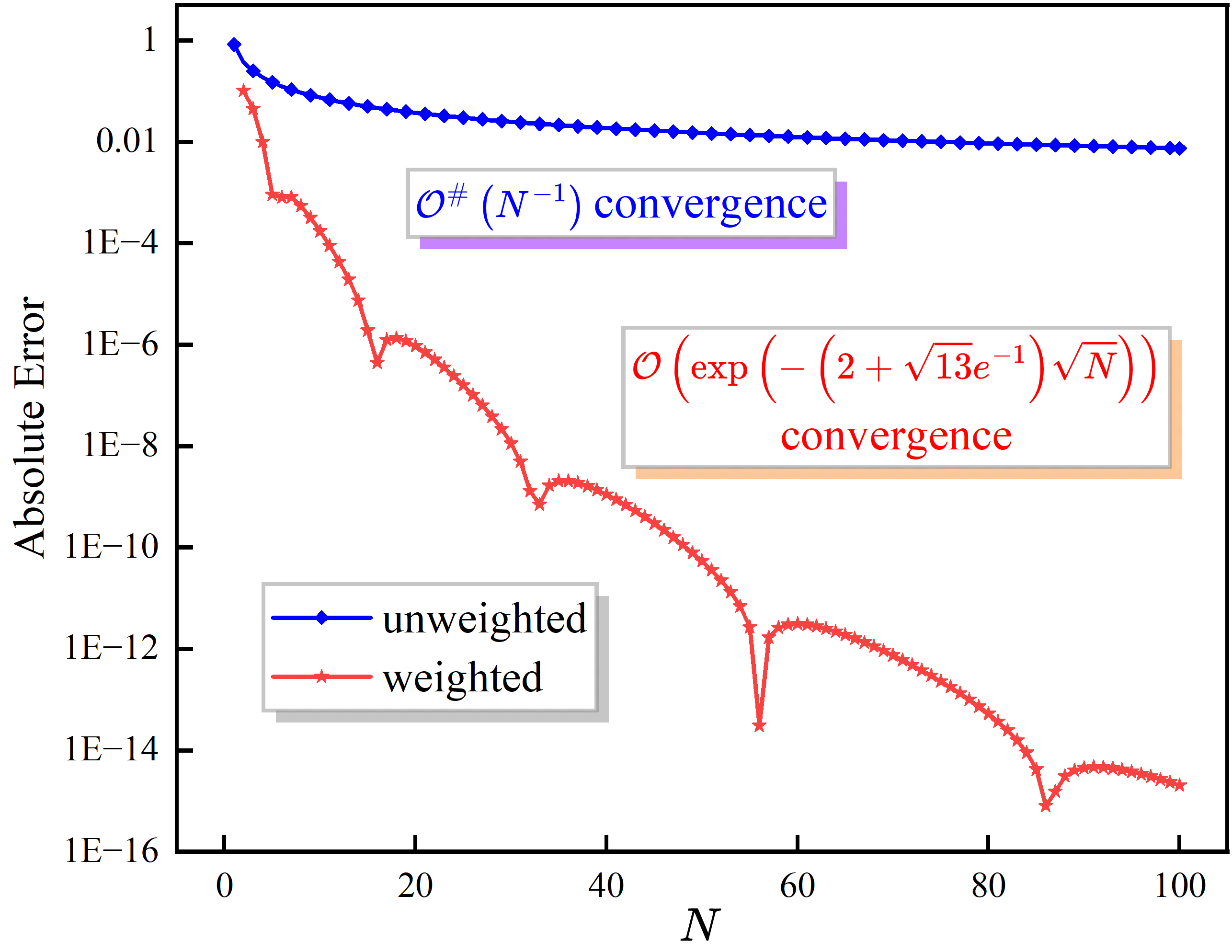
8 Numerical simulation and analysis of convergence rates

In this section, we present an example to illustrate our quantitative estimates of the convergence rates as stated in Theorem 1.1. Let the decaying parameter be λ=2\lambda=2, the rotating parameter be ρ=3\rho=3, and the initial phase parameter be θ=1\theta=1. In this case,

DWN(2,3,1)=1Nn=0N1e2nsin(1+3n),WDWN(2,3,1)=1ANn=0N1w(n/N)e2nsin(1+3n).{{\rm{DW}}_{N}}\left({2,3,1}\right)=\frac{1}{N}\sum\limits_{n=0}^{N-1}{{e^{-2n}}\sin\left({1+3n}\right)},\;\;{\rm{WDW}}_{N}\left({2,3,1}\right)=\frac{1}{{{A_{N}}}}\sum\limits_{n=0}^{N-1}{w\left({n/N}\right){e^{-2n}}\sin\left({1+3n}\right)}.

It can be verified that eλsin(ρθ)+sinθ=e2sin2+sin10.960{e^{-\lambda}}\sin\left({\rho-\theta}\right)+\sin\theta={e^{-2}}\sin 2+\sin 1\approx 0.96\neq 0, and

ξ=ξ(λ,ρ)=2λ+e1λ2+ρ𝕋2=2+13e1.\xi=\xi(\lambda,\rho)=\sqrt{2\lambda}+{e^{-1}}\sqrt{{\lambda^{2}}+\left\|\rho\right\|_{\mathbb{T}}^{2}}=2+\sqrt{13}{e^{-1}}.

Therefore, Theorem 1.1 tells us that the unweighted average DWN(2,3,1){{\rm{DW}}_{N}}\left({2,3,1}\right) exhibits polynomial convergence of 𝒪#(N1)\mathcal{O}^{\#}\left(N^{-1}\right), while the weighted average WDWN(2,3,1){\rm{WDW}}_{N}\left({2,3,1}\right) demonstrates exponential convergence as given by

𝒪(exp(ξN))=𝒪(exp((2+13e1)N)).\mathcal{O}\left({\exp\left({-\xi\sqrt{N}}\right)}\right)=\mathcal{O}\left({\exp\left({-\left({2+\sqrt{13}{e^{-1}}}\right)\sqrt{N}}\right)}\right). (8.1)

We would like to emphasize that (8.1) is exceptionally precise. For N=100N=100, (8.1) provides an upper bound on the absolute error of approximately 3.58×10153.58\times{10^{-15}}, while the actual error is around 2.04×10152.04\times{10^{-15}}, as illustrated in Figure 1; for N=1000N=1000, (8.1) yields an upper bound on the absolute error of approximately 2.07×10462.07\times{10^{-46}}, compared to the actual error of approximately 2.11×10472.11\times{10^{-47}}, however, due to the extremely small nature of these values, they are not provided in the figure.

Refer to caption
Figure 1: Comparison of the convergence rates

Actually, on the standard torus 𝕋=/2π\mathbb{T}=\mathbb{R}/2\pi\mathbb{Z}, the rotation number with respect to the rotating parameter in this case is 3/2π3/2\pi, which admits a Diophantine exponent of δ=6.11\delta=6.11***Indeed, for any irrational xx with an exact Diophantine exponent, ax+bcx+d\frac{{ax+b}}{{cx+d}} admits the same exact Diophantine exponent as xx, provided that a,b,c,da,b,c,d are rational and adbc0ad-bc\neq 0. As a consequence, 32π\frac{3}{{2\pi}} admits the same exact Diophantine exponent as π\pi, as seen in the equivalent expression 32π+1=2π+32π+0\frac{3}{{2\pi}}+1=\frac{{2\pi+3}}{{2\pi+0}}., i.e.,

|q32πp|>C|q|δ,q+,p\left|{q\cdot\frac{3}{{2\pi}}-p}\right|>\frac{C}{{{{\left|q\right|}^{\delta}}}},\;\;\forall q\in{\mathbb{N}^{+}},\;\;\forall p\in\mathbb{Z}

for some C>0C>0, see Zeilberger and Zudilin [41] for a more accurate estimate on this aspect. We intentionally avoided using the constant type (with exact Diophantine exponent 22It is well known that such rotation numbers only form a set of zero Lebesgue measure in \mathbb{R}.) rotation numbers that would have further accelerated the convergence rate. Instead, we select a less irrational (more universal) alternative as 3/2π3/2\pi. We also refer to Das et al. [6] for a numerical comparison of the two cases in the weighted Birkhoff average with rotation numbers π3\pi-3 (having the same Diophantine exponent as 3/2π3/2\pi) and 21\sqrt{2}-1 (the constant type).

Acknowledgements

This work was supported in part by National Basic Research Program of China (Grant No. 2013CB834100), National Natural Science Foundation of China (Grant Nos. 12071175, 11171132, 11571065, 12471183), Project of Science and Technology Development of Jilin Province (Grant Nos. 2017C028-1, 20190201302JC), and Natural Science Foundation of Jilin Province (Grant No. 20200201253JC). The first author was deeply grateful to Professors Wolfgang M. Schmidt, Paul Vojta, Doron Zeilberger, Wadim Zudilin for their valuable email assistance on Diophantine approximation, and Maximilian Ruth and David Bindel for their valuable email discussions on the accurate convergence rates in weighted Birkhoff averages.

References

  • [1] V. Arnold, Ordinary differential equations. Springer-Verlag, Berlin, 1992. pp. 334.
  • [2] A. Belotto da Silva, E. Bierstone, A. Kiro, Sharp estimates for blowing down functions in a Denjoy-Carleman class. Int. Math. Res. Not. IMRN 2022, pp. 9685–9707. https://doi.org/10.1093/imrn/rnaa367
  • [3] D. Blessing, J. D. Mireles James, Weighted Birkhoff Averages and the Parameterization Method. arXiv:2306.16597
  • [4] R. Calleja, A. Celletti, J. Gimeno, R. de la Llave, Accurate computations up to breakdown of quasi-periodic attractors in the dissipative spin-orbit problem. J. Nonlinear Sci. 34 (2024), Paper No. 12, pp. 38. https://doi.org/10.1007/s00332-023-09988-w
  • [5] S. Das, J. Yorke, Super convergence of ergodic averages for quasiperiodic orbits. Nonlinearity 31 (2018), pp. 491–501. https://doi.org/10.1088/1361-6544/aa99a0
  • [6] S. Das, Y. Saiki, E. Sander, J. Yorke, Quantitative quasiperiodicity. Nonlinearity 30 (2017), pp. 4111–4140. https://doi.org/10.1088/1361-6544/aa84c2
  • [7] D. Dolgopyat, B. Fayad, Deviations of ergodic sums for toral translations II. Boxes. Publ. Math. Inst. Hautes Études Sci. 132 (2020), pp. 293–352. https://doi.org/10.1007/s10240-020-00120-2
  • [8] N. Duignan, J. D. Meiss, Nonexistence of invariant tori transverse to foliations: an application of converse KAM theory. Chaos 31 (2021), Paper No. 013124, pp. 19. https://doi.org/10.1063/5.0035175
  • [9] N. Duignan, J. D. Meiss, Distinguishing between regular and chaotic orbits of flows by the weighted Birkhoff average, Phys. D 449 (2023), Paper No. 133749, pp. 16. https://doi.org/10.1016/j.physd.2023.133749
  • [10] G. Forni, Deviation of ergodic averages for area-preserving flows on surfaces of higher genus. Ann. of Math. (2) 155 (2002), pp. 1–103. https://doi.org/10.2307/3062150
  • [11] L. Grafakos, Classical Fourier analysis. Third edition. Graduate Texts in Mathematics, 249. Springer, New York, 2014. xviii+638 pp.
  • [12] M.-R. Herman, Sur la conjugaison différentiable des difféomorphismes du cercle à des rotations, Inst. Hautes Études Sci. Publ. Math., 49 (1979), pp. 5–233. http://www.numdam.org/item?id=PMIHES_1979__49__5_0
  • [13] A. Kachurovskiĭ, Rates of convergence in ergodic theorems. (Russian) Uspekhi Mat. Nauk 51 (1996), pp. 73–124; translation in Russian Math. Surveys 51 (1996), pp. 653–703. https://doi.org/10.1070/RM1996v051n04ABEH002964
  • [14] Y. Katznelson, An introduction to harmonic analysis. Third edition. Cambridge Mathematical Library. Cambridge University Press, Cambridge, 2004. xviii+314 pp. https://doi.org/10.1017/CBO9781139165372
  • [15] V. V. Kozlov, On the ergodic theory of equations of mathematical physics. Russ. J. Math. Phys. 28 (2021), pp. 73–83. https://doi.org/10.1134/S1061920821010088
  • [16] U. Krengel, On the speed of convergence in the ergodic theorem. Monatsh. Math. 86 (1978/79), pp. 3–6. https://doi.org/10.1007/BF01300052
  • [17] J. Laskar, Frequency analysis for multi-dimensional systems. Global dynamics and diffusion. Phys. D 67 (1993), pp. 257–281. https://doi.org/10.1016/0167-2789(93)90210-R
  • [18] J. Laskar, Frequency analysis of a dynamical system. Qualitative and quantitative behaviour of planetary systems (Ramsau, 1992). Celestial Mech. Dynam. Astronom. 56 (1993), pp. 191–196. https://doi.org/10.1007/BF00699731
  • [19] J. Laskar, Introduction to frequency map analysis. Hamiltonian systems with three or more degrees of freedom (S’Agaró, 1995), pp. 134–150, NATO Adv. Sci. Inst. Ser. C: Math. Phys. Sci., 533, Kluwer Acad. Publ., Dordrecht, 1999.
  • [20] G. Liu, Y. Li, X. Yang, Existence and multiplicity of rotating periodic solutions for resonant Hamiltonian systems. J. Differential Equations 265 (2018), pp. 1324–1352. https://doi.org/10.1016/j.jde.2018.04.001
  • [21] G. Liu, Y. Li, X. Yang, Existence and multiplicity of rotating periodic solutions for Hamiltonian systems with a general twist condition. J. Differential Equations 369 (2023), pp. 229–252. https://doi.org/10.1016/j.jde.2023.06.001
  • [22] J. D. Meiss, E. Sander, Birkhoff averages and the breakdown of invariant tori in volume-preserving maps. Phys. D 428 (2021), Paper No. 133048, pp. 20. https://doi.org/10.1016/j.physd.2021.133048
  • [23] R. Montalto, M. Procesi, Linear Schrödinger equation with an almost periodic potential. SIAM J. Math. Anal. 53 (2021), pp. 386–434. https://doi.org/10.1137/20M1320742
  • [24] I. Podvigin, On the pointwise rate of convergence in the Birkhoff ergodic theorem: recent results. Ergodic Theory and Dynamical Systems: Proceedings of the Workshops University of North Carolina at Chapel Hill 2021, edited by Idris Assani, Berlin, Boston: De Gruyter, 2024, pp. 117–126. https://doi.org/10.1515/9783111435503-005
  • [25] M. Ruth, D. Bindel, Finding Birkhoff Averages via Adaptive Filtering. https://arxiv.org/abs/2403.19003
  • [26] D. Salamon, The Kolmogorov-Arnold-Moser theorem. Math. Phys. Electron. J. 10 (2004), Paper 3, pp. 37.
  • [27] E. Sander, J. D. Meiss, Birkhoff averages and rotational invariant circles for area-preserving maps. Phys. D 411 (2020), 132569, pp. 19. https://doi.org/10.1016/j.physd.2020.132569
  • [28] E. Sander, J. D. Meiss, Rotation Vectors for Torus Maps by the Weighted Birkhoff Average. https://arxiv.org/abs/2310.11600
  • [29] E. Sander, J. D. Meiss, Computing Lyapunov Exponents using Weighted Birkhoff Averages. https://arxiv.org/abs/2409.08496
  • [30] E. Stein, R. Shakarchi, Fourier analysis. An introduction. Princeton Lectures in Analysis, 1. Princeton University Press, Princeton, NJ, 2003. xvi+311 pp.
  • [31] S. Sternberg, Local contractions and a theorem of Poincaré. Amer. J. Math. 79 (1957), pp. 809–824. https://doi.org/10.2307/2372437
  • [32] S. Sternberg, On the structure of local homeomorphisms of euclidean nn-space. II. Amer. J. Math. 80 (1958), pp. 623–631. https://doi.org/10.2307/2372774
  • [33] Z. Tong, Y. Li, Exponential convergence of the weighted Birkhoff average. J. Math. Pures Appl. (9) 188 (2024), pp. 470–492. https://doi.org/10.1016/j.matpur.2024.06.003
  • [34] Z. Tong, Y. Li, A note on exponential convergence of Cesàro weighted Birkhoff average and multimodal weighted approach. To appear in Acta Math. Sin. (Engl. Ser.).
  • [35] Z. Tong, Y. Li, Universal exponential pointwise convergence for weighted multiple ergodic averages over 𝕋\mathbb{T}^{\infty}. https://arxiv.org/abs/2405.02866
  • [36] V. V. Ryzhikov, Slow convergences of ergodic averages. (Russian) Mat. Zametki 113 (2023), pp. 742–746; translation in Math. Notes 113 (2023), pp. 704–707. https://doi.org/10.4213/sm9844
  • [37] S. Wang, Y. Li, X. Yang, Synchronization, symmetry and rotating periodic solutions in oscillators with Huygens’ coupling. Phys. D 434 (2022), Paper No. 133208, pp. 22. https://doi.org/10.1016/j.physd.2022.133208
  • [38] J. Xing, X. Yang, Y. Li, Lyapunov center theorem on rotating periodic orbits for Hamiltonian systems. J. Differential Equations 363 (2023), pp. 170–194. https://doi.org/10.1016/j.jde.2023.03.016
  • [39] J.-C. Yoccoz, Sur la disparition de propriétés de type Denjoy-Koksma en dimension 22. C. R. Acad. Sci. Paris Sér. A–B 291 (1980), pp. A655–A658.
  • [40] J.-C. Yoccoz, Centralisateurs et conjugaison différentiable des difféomorphismes du cercle. Petits diviseurs en dimension 11. Astérisque No. 231 (1995), pp. 89–242.
  • [41] D. Zeilberger, W. Zudilin, The irrationality measure of π\pi is at most 7.103205334137…. Mosc. J. Comb. Number Theory 9 (2020), pp. 407–419. https://doi.org/10.2140/moscow.2020.9.407
  • [42] W. Zhang, K. Lu, W. Zhang, Differentiability of the conjugacy in the Hartman-Grobman theorem. Trans. Amer. Math. Soc. 369 (2017), pp. 4995–5030. https://doi.org/10.1090/tran/6810
  • [43] A. Zygmund, Trigonometric series. 2nd ed. Vols. I, II. Cambridge University Press, New York, 1959. Vol. I. pp. xii+383; Vol. II. pp. vii+354.