Quantum Circuit Distillation and Compression

Shunsuke Daimon daimon.shunsuke@qst.go.jp Department of Applied Physics, The University of Tokyo, Tokyo 113-8656, Japan. Department of Applied Physics and Physico-Informatics, Keio University, Yokohama 223-8522, Japan. Institute for AI and Beyond, The University of Tokyo, Tokyo 113-8656, Japan. Quantum Materials and Applications Research Center, National Institutes for Quantum Science and Technology, Tokyo 152-8550, Japan. Kakeru Tsunekawa Department of Applied Physics, The University of Tokyo, Tokyo 113-8656, Japan. Ryoto Takeuchi Department of Applied Physics, The University of Tokyo, Tokyo 113-8656, Japan. Takahiro Sagawa Department of Applied Physics, The University of Tokyo, Tokyo 113-8656, Japan. Naoki Yamamoto Department of Applied Physics and Physico-Informatics, Keio University, Yokohama 223-8522, Japan. Eiji Saitoh Department of Applied Physics, The University of Tokyo, Tokyo 113-8656, Japan. Department of Applied Physics and Physico-Informatics, Keio University, Yokohama 223-8522, Japan. Institute for AI and Beyond, The University of Tokyo, Tokyo 113-8656, Japan. Institute for Materials Research, Tohoku University, Sendai 980-8577, Japan. WPI Advanced Institute for Materials Research, Tohoku University, Sendai 980-8577, Japan.

Abstract

Quantum coherence in a qubit is vulnerable to environmental noise. When long quantum calculation is run on a quantum processor without error correction, the noise often causes fatal errors and messes up the calculation. Here, we propose quantum-circuit distillation to generate quantum circuits that are short but have enough functions to produce an output almost identical to that of the original circuits. The distilled circuits are less sensitive to the noise and can complete calculation before the quantum coherence is broken in the qubits. We created a quantum-circuit distillator by building a reinforcement learning model, and applied it to the inverse quantum Fourier transform (IQFT) and Shor’s quantum prime factorization. The obtained distilled circuit allows correct calculation on IBM-Quantum processors. By working with the quantum-circuit distillator, we also found a general rule to generate quantum circuits approximating the general $n$ -qubit IQFTs. The quantum-circuit distillator offers a new approach to improve performance of noisy quantum processors.

I Introduction

Quantum calculation has been performed on gate-type quantum processors by designing a sequence of quantum logic gates called a quantum circuitLadd et al. (2010); Alexeev et al. (2021). Numerous algorithms based on quantum circuits have theoretically been proposed to realize quantum computationNielsen and Chuang (2010); Montanaro (2016). However, existing quantum processors are too noisy and not yet ready to perform these quantum algorithms properlyPreskill (2018); Córcoles et al. (2019). The noise causes errors in running quantum circuits and prevents the circuits from working properlyChow et al. (2012); Willsch et al. (2017), and the quantum processors cannot even perform simple quantum algorithms.

Here, we propose a quantum-circuit distillator to generate a quantum circuit that is short but has enough functions to yield almost the same output distribution as that of a long original quantum circuit. We show that the quantum-circuit distillator enables existing quantum processors to work properly by reducing errors effectively by demonstrating the distillation of the IQFT and Shor’s integer factorization circuits. By extrapolating the outputs from the distillator, we also found approximated general $n$ -qubit IQFTs for any qubit number $n$ .

II Results and Discussion

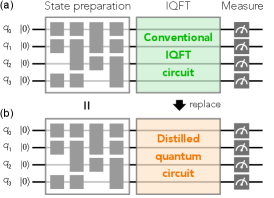
First, we show a result of the conventional four-qubit IQFT obtained with an existing superconducting quantum computer IBM Quantum (IBMQ)Gambetta et al. (2017); Wendin (2017); IBM . Figure 1(a) shows the conventional quantum circuit for the four-qubit IQFTNielsen and Chuang (2010). By applying the circuit to an initial quantum state and measuring the final state, the IBMQ outputs a four-digit bitstring. By repeating the measurement, we obtained probability distribution of the bitstrings. Figure 1(e) shows an output distribution profile for the four-qubit IQFT obtained from IBMQ. On the other hand, Fig. 1(d) shows the exact analytical result of the four-qubit IQFT calculation for the same input. The distribution observed experimentally from IBMQ [Fig. 1(e)] is far different from the expected distribution [Fig. 1(d)], showing that the conventional quantum circuit is too long to properly work on IBMQ due to the noise.

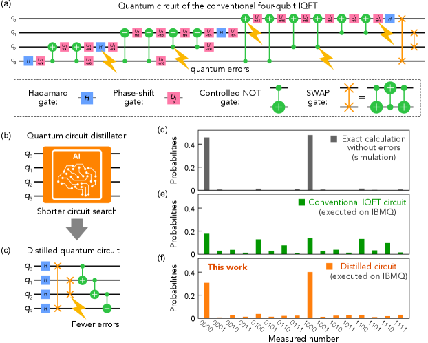
Refer to caption — Figure 1: (a) A quantum circuit for the inverse quantum Fourier transform (IQFT) for four qubits $q_{0}$ , $q_{1}$ , $q_{2}$ , and $q_{3}$ . The blue, red, green, and orange components represent the Hadamard, phase-shift, controlled NOT, and SWAP gates, respectively. (b) Schematic of a quantum circuit search. (c) A distilled quantum circuit for the four-qubit IQFT generated from the distillator. (d) A probability distribution obtained from the exact IQFT calculation without errors. (e), (f) Probability distributions obtained from the quantum computer IBMQ for the conventional four-qubit IQFT circuit (e) and for the distilled quantum circuit (f).

Before showing the details of the distillator developed in the present study, we demonstrate how it works. When our distillator is applied to the four-qubit IQFT [Fig. 1(b)], it compresses the conventional IQFT circuit and outputs a distilled brief quantum circuit as shown in Fig. 1(c). We can carry out IQFT calculation using the obtained circuit. Figure 1(f) shows the probability distribution of the four-qubit IQFT obtained from the distilled quantum circuit for the same input as those in Fig. 1(d) and (e). Significantly, the output profile is almost the same as the exact calculation [Fig. 1(d)]; the four-qubit IQFT is successfully completed in spite of the noisy qubit environment in IBMQ owing to the distillation. The distilled quantum circuit is four times shorter than the conventional quantum circuit with 36 quantum gates, and the brevity is responsible for the fewer errors and the successful calculation.

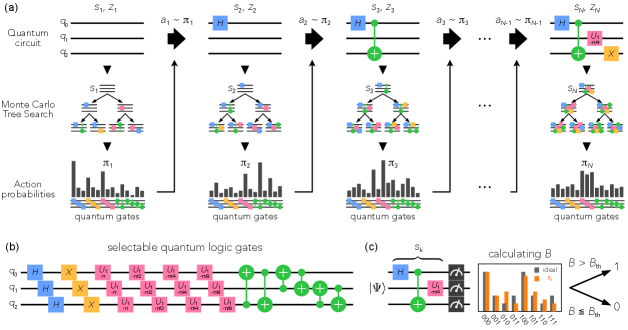
The main concept of the quantum-circuit distillator is to compress a target quantum circuit into a shorter quantum circuit that well approximates input/output relation of the target quantum circuit. To realize such a distillator, it is necessary to search an ideal quantum circuit from a huge number of combinations of quantum logic gates. We addressed this problem by taking advantage of the remarkable searching abilities of reinforcement learningKaelbling et al. (1996); Arulkumaran et al. (2017), known to be suitable for solving optimization problems for finite element combinations, such as quantum gates. To construct a reinforcement learning model for quantum circuit compression, we designed a variable-length quantum circuit search based on the Monte-Carlo tree search in which a deep neural network is used to accelerate the tree searchSilver et al. (2017a, b) (see Appendixes D and E and Figs. A·3 and A·4 for more details). In contrast to the quantum circuit search using fixed-length quantum circuitsPeruzzo et al. (2014); Farhi et al. (2014); Endo et al. (2021); Cerezo et al. (2021); Nakaji et al. (2022), such as the quantum circuit learningMitarai et al. (2018), our model enables us to search quantum circuits with different lengths and different circuit structures. The deep neural network makes the quantum circuit search efficient by sequentially predicting the most suitable gate to be placed next to the gate array constructed so far in the tree search.

We found that the Bhattacharyya coefficientFuchs and Van De Graaf (1999) $B$ works well as a reward function in the reinforcement learning used in the quantum-circuit distillation. The Bhattacharyya coefficient $B$ is a classical expression of the quantum fidelity, which gives a measure for the similarity between two quantum circuits based on the probability distributions (see Appendix A for the definition of $B$ ). $B$ takes a value between 0 and 1, and approaches 1 (0) when the two probability distributions are the same (dissimilar). The quantum gate fidelityFuchs and Van De Graaf (1999), which compares quantum circuits as unitary transformations, has often been used as a reward function in the previous studies on quantum circuit searchKhaneja et al. (2005); Khatri et al. (2019); Dalgaard et al. (2020); Peng et al. (2020); Magann et al. (2021); Fösel et al. (2021); Moro et al. (2021); Kimura et al. (2022). However, we found that it imposes too strong constraints to the search in the present reinforcement learning [see Fig. 3(e)]. On the other hand, $B$ only compares probability distributions obtained from quantum circuits and makes it easier to find optimal circuits among a large number of quantum gate combinations.

By applying the developed quantum-circuit distillator using the reinforcement learning to the four-qubit IQFT circuit shown in Fig. 1(a), we obtained the distilled IQFT circuit shown in Fig. 1(c). As we discussed above, the distilled circuit outputs the probability distribution shown in Fig. 1(f) for an input, and the distribution is almost the same as the exact calculation shown in Fig. 1(d), greatly improved from the original IQFT circuit [Fig. 1(e)]. By comparing the probability distributions obtained from the distilled circuit [Fig. 1(f)] and the exact calculation [Fig. 1(d)], we obtained the $B$ value of 0.91. In contrast, for the probability distribution obtained from the conventional quantum circuit shown in Fig. 1(e), $B$ takes a lower value, 0.69, demonstrating the superiority of the distilled circuit.

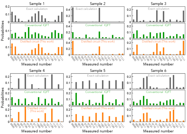
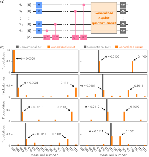
We confirmed the generalization performance of the present reinforcement learning in the circuit distillator; we found that the distilled quantum circuit shown in Fig. 1(c) well reproduces the exact calculation of the four-qubit IQFT also for the input quantum states not used for the learning (see Appendix C for the theoretical analysis of the distilled quantum circuit). Figure 2 shows output probability distributions for several input quantum states prepared by random sequences of quantum gates. All the outputs from the distilled quantum circuit (orange bars in Fig. 2) well reproduce the exact calculations (gray bars in Fig. 2), while the outputs from the conventional IQFT circuit (green bars in Fig. 2) are far from the exact calculations (gray bars in Fig. 2).

We calculated the average value of the Bhattacharyya coefficient $B_{\rm{ave}}$ for randomly initialized input quantum states; we prepared input states by randomly applying quantum logic gates to the ground state of the quantum bits, and then the distilled quantum circuit is applied to the initial states (see Appendix A and Fig. A·1). $B_{\rm{ave}}$ for the distilled four-qubit IQFT circuit was estimated to be $\sim$ 0.93, which is greater than that for the conventional circuit 0.90. The result shows again that the distilled quantum circuit with fewer quantum gates generates better outputs than the longer circuit derived from the exact quantum algorithm.

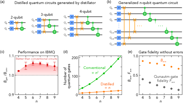
By exploiting some outputs from the quantum-circuit distillator, we can infer general quantum circuits which can approximate the $n$ -qubit IQFTs for any natural number $n$ , as follows. In Fig. 3(a), we show distilled circuits obtained from our distillator for the 2-, 3-, and 4-qubit IQFTs. By comparing these distilled quantum circuits shown in Fig. 3(a), we found a regularity on the array of the quantum gates: the gates are arranged in the order of Hadamard, SWAP, and CNOT gates in the distilled circuits [compare the distilled 2-, 3- , and 4-qubit IQFTs in Fig. 3(a)]. From the observation, we inductively predicted approximate quantum circuits generalized to arbitrary $n$ as shown in Fig. 3(b). We found that the generalized quantum circuits actually well approximate the conventional $n$ -qubit IQFT even for $n$ greater than four. The averaged Bhattacharyya coefficients for the generalized circuits were found to be greater than that for the conventional IQFT circuits even for $n$ greater than four as shown in Fig. 3(c). The result demonstrates that the generalized circuits outperform the conventional IQFT circuits on the existing quantum computer IBMQ. As shown in Fig. 3(d), the generalized quantum circuits reduce the number of the gates from $O(n^{2})$ to $O(n)$ compared to the conventional IQFTsNielsen and Chuang (2010). The number of gates is less than that of an approximation circuit $O(n\log n)$ proposed in previous studiesBarenco et al. (1996); Nam et al. (2020). The gate number reduction mitigates errors in computation and contributes to the performance of the generalized circuits. Note that the generalized circuits do not approximate the IQFT in terms of unitary transformations while they approximate the output probability distributions. As shown in Fig. 3(e), while the output probability distributions show high values of $B_{\rm{ave}}$ , the quantum gate fidelity $F_{\rm{ave}}$ takes much lower values for all $n$ . If the quantum gate fidelity is used as a reward for the search, as in previous studiesFösel et al. (2021); Moro et al. (2021), the distilled circuit cannot be found. In addition, we have succeeded in analytically justifying the generalized approximate quantum circuits for a special case as described in Appendix C.

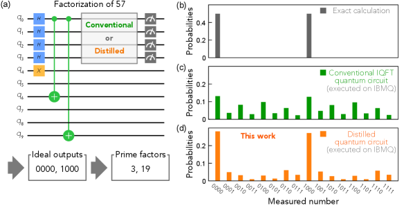
Finally, we demonstrate the application of the distilled IQFT circuit to executing Shor’s integer factorizationNielsen and Chuang (2010); Ekert and Jozsa (1996) of 57. Figure 4(a) shows the conventional quantum circuit for the factorization. The quantum circuit ideally outputs 0000 or 1000 [Fig. 4(b)] for the input of 57, and the prime factors of 3 and 19 can be derived from the output numbers. When the conventional quantum circuit is run on the quantum computer IBMQ, the output distribution profile [Fig. 4(c)] is far different from the exact calculation [Fig. 4(b)], and the desired numbers are no longer outputted as shown in Fig. 4(c). On the other hand, by replacing the IQFT with the distilled quantum circuit, we obtained almost the same distribution profile as the exact calculation [compare Fig. 4(b) and (d)]. The result shows that the distilled quantum circuits enable Shor’s integer factorization on the system.

III Conclusion

In summary, we proposed and demonstrated a quantum-circuit distillator to generate quantum circuits less sensitive to noise in existing quantum processors. We applied the quantum-circuit distillator to the four-qubit IQFT and demonstrated that the generated distilled quantum circuit outperforms the conventional IQFT circuit on an existing quantum computer IBMQ. The distilled quantum circuits also let us discover the generalized quantum circuits approximating the general $n$ -qubit IQFTs. The result shows a new direction of scientific research, in which humans and machine learning work together to create knowledge. Our method has a wide range of applications, including not only distillation of quantum algorithms such as IQFT, but also data encoding for quantum machine learning. This work will accelerate the realization of valuable quantum computations for practical tasks.

Acknowledgements.

The authors thank N. Yokoi for valuable discussions. This work was supported by ERATO (No. JPMJER1402), CREST (Nos. JPMJCR20C1, JPMJCR20T2) from JST, Japan; Grant-in-Aid for Scientific Research (S) (No. JP19H05600), Grant-in-Aid for Research Activity Start-up (No. JP19K21035), Grant-in-Aid for Transformative Research Areas (No. JP22H05114) from JSPS KAKENHI, Japan. T.S. is supported by JST ERATO-FS (No. JPMJER2204). N.Y. is supported by MEXT Quantum Leap Flagship Program (Nos. JPMXS0118067285, JPMXS0120319794). We acknowledge the use of IBM Quantum services for this work as part of the IBM Quantum Hub at The University of Tokyo and Keio University. The views expressed are those of the authors and do not reflect the official policy or position of IBM or the IBM Quantum team.

Appendix A Performance estimation of quantum circuits

Performance of a quantum circuit on a quantum processor is estimated by calculating $B$ between the output probabilities from the quantum circuit $p_{\rm{qc}}$ and the correct answer $p_{\rm{ans}}$ calculated from the ideal IQFT for an initial quantum state $\left|\Psi\right>$ . The initial quantum state is prepared by applying a random sequence of quantum gates $g_{1},g_{2},\cdots,g_{m}$ to the zero state $\left|0\right>:\left|\Psi\right>=g_{m}\cdots g_{2}g_{1}\left|0\right>$ , where $g_{1},g_{2},\cdots,g_{m}$ are selected from the Hadamard, NOT, Phase-shift, and CNOT gates. Figure A·3(b) shows an example of quantum gates used for the initialization of 3-qubit quantum states. The number of the quantum gates for the initialization $m$ is set to $4n$ for $n$ -qubit quantum circuits in our calculation. Next, the $\left|\Psi\right>$ is transformed by the quantum circuit and measured [Fig. A·1(b)]. By repeating the measurement, we obtain the probability distribution $p_{\rm{qc}}$ for the input quantum state $\left|\Psi\right>$ . At the same time, we numerically calculate the IQFT for the input quantum state $\left|\Psi\right>$ and obtained the probability distribution $p_{\rm{ans}}$ [Fig. A·1(a)]. Then, $B(p_{\rm{qc}},p_{\rm{ans}})=\sum_{i\in\Omega}\sqrt{p_{\rm{qc}}(i)p_{\rm{ans}}(i)}$ is calculated, where $\Omega$ is the set of the observed binary numbers for the $n$ -qubit quantum circuits. By changing the initialization gates and repeating the $B$ calculation for many input quantum states, $B_{\rm{ave}}$ is obtained as the average value of $B$ for the input quantum states.

Appendix B Devices and its noise parameters used in the performance estimation

The calculation results shown in Figs. 1 and 2 were obtained from the quantum computer IBMQ Vigo, where the average relaxation times $T_{1}$ and $T_{2}$ , and readout error rate are about $8\times 10^{1}$ $\mu$ s, $7\times 10^{1}$ $\mu$ s, and $3\times 10^{-2}$ , respectively. The results shown in Fig. 3(c) were obtained from the quantum computer IBMQ Melbourne, where the average relaxation times $T_{1}$ and $T_{2}$ and readout error rate are about $6\times 10^{1}$ $\mu$ s, $6\times 10^{1}$ $\mu$ s, and $5\times 10^{-2}$ , respectively. The results shown in Fig. 4 were obtained from the quantum computer IBMQ Sydney, where the average relaxation times $T_{1}$ and $T_{2}$ and readout error rate are about $1\times 10^{2}$ $\mu$ s, $8\times 10^{1}$ $\mu$ s, and $3\times 10^{-2}$ , respectively.

Appendix C Quantum phase estimation using the generalized $n$ -qubit quantum circuits

The generalized $n$ -qubit quantum circuit shown in Fig. 3(b) was found to work well in the quantum phase estimation (QPE) problemNielsen and Chuang (2010); Aspuru-Guzik et al. (2005). The QPE is a quantum algorithm to estimate the phase $\theta$ for a unitary matrix, $U$ , and its eigen quantum state $\left|\phi\right>$ such that $U\left|\phi\right>=e^{2\pi i\theta}\left|\phi\right>$ . The QPE is performed by the following three steps. Firstly, a product state $\left|0\right>\otimes\left|\phi\right>$ is prepared. Secondly, the Hadamard and controlled phase-shift gates are applied to the state as shown in Fig. A·2(a), and the phase $\theta$ is introduced to the quantum state: $1/\sqrt{2^{n}}\sum_{k=0}^{2^{n}-1}e^{2\pi i\theta k}\left|k\right>\otimes\left|\phi\right>$ , where $k$ denotes the integer representation of $n$ -bit binary numbers. Thirdly, the IQFT is applied, and the state is converted into $\left|2^{n}\theta\right>\otimes\left|\phi\right>$ , where we assume that $2^{n}\theta$ is an integer for simplicity. Then, we can obtain $\theta$ by measuring the quantum state. Here, we replace the IQFT with the generalized $n$ -qubit quantum circuit shown in Fig. 3(b), and we obtain the final quantum state as $\sum_{j_{1},\cdots,j_{n}\in\{0,1\}}E_{n}^{0\oplus j_{1}}E_{n-1}^{j_{1}\oplus j_{2}}\cdots E_{1}^{j_{n-1}\oplus j_{n}}\left|j_{n}\cdots j_{2}j_{1}\right>$ , where $E_{k}^{0}=\left(1+e^{i\pi 2^{k}\theta}\right)/2$ and $E_{k}^{1}=\left(1-e^{i\pi 2^{k}\theta}\right)/2$ , $\oplus$ symbol denotes the exclusive disjunction between two binary digits. The probability that the state $\left|j_{n}\cdots j_{2}j_{1}\right>$ is observed is $\left|E_{n}^{0\oplus j_{1}}E_{n-1}^{j_{1}\oplus j_{2}}\cdots E_{1}^{j_{n-1}}\right|^{2}$ . We analytically proved that the probability takes the maximum value when $j_{n}\cdots j_{2}j_{1}$ is the binary representation of $2^{n}\theta$ or $2^{n}-2^{n}\theta$ [Fig. A·2(b)]. The result means that the generalized $n$ -qubit quantum circuit outputs the correct answer with the maximum probability at least in the QPE. Here, we note that the probability of obtaining the correct answer decreases exponentially with increasing the number of qubits. The generalized quantum circuits cannot solve the QPE in polynomial time with bounded error probability.

Appendix D Reinforcement learning model

We formulated the search problem as combination optimization of quantum logic gates. We have applied reinforcement learning Arulkumaran et al. (2017) to the problem by treating quantum circuits and appending one quantum gate to the end of the quantum circuit as states and action, respectively [Fig. A·3(a)]. A state $s_{k}$ consisting of $k$ quantum gates is updated to a state $s_{k+1}$ consisting of $k+1$ quantum gates by applying an action $a_{k}$ . The quantum gates are selected from the Hadamard, NOT, Phase-shift, and CNOT gates, where magnitude of the phase shift is selected from $-2\pi/2^{1}$ , $-2\pi/2^{2}$ , $-2\pi/2^{3}$ , or $-2\pi/2^{4}$ to construct a universal gate set. For example, we prepared 24 quantum gates for constructing 3-qubit quantum circuits as shown in Fig. A·3(b). Then, various quantum circuits with different lengths and different combinations of quantum gates can be generated depending on a series of actions. $a_{k}$ is selected by using the action probability functions ${\boldsymbol{\pi}}(s_{k})$ Kaelbling et al. (1996) obtained from the Monte-Carlo tree search (MCTS)Silver et al. (2017a, b) (see Fig. A·3). The component of the ${\boldsymbol{\pi}}(s_{k})$ is defined as ${\boldsymbol{\pi}}(s_{k},a)={\rm{Pr}}(a|s_{k})$ , where $a$ is an action. The reward $z_{k}$ for the reinforcement learning is determined by calculating the Bhattacharyya coefficient $B_{k}$ between the output probabilities from $s_{k+1}$ and the correct answer [Fig. A·3(c)]. When $B_{k}$ is above a threshold value, $B_{\rm{th}}$ , for several input quantum states, we substitute 1 for $z_{k}$ and abort the search. When $B_{k}$ is less than $B_{\rm{th}}$ , we assign 0 to $z_{k}$ and repeat searching for the next action, updating the state, and comparing $B_{k+1}$ and $B_{\rm{th}}$ . If no states satisfy the condition until $k$ reaches the upper limit $N$ , we assign -1 to $z_{N}$ . $N$ determines the maximum length of the quantum circuits in the search, and we set $N$ to around $4n$ in this study. The total reward $z$ for the search is defined as the sum of the rewards $z=\sum_{k}z_{k}$ . The obtained set $(s_{k},{\boldsymbol{\pi}}(s_{k}),z)$ is used as the training data to update the MCTS and dual neural network as explained below.

The reinforcement learning aims to learn a policy so as to maximize the total reward. As the policy model, we used the Alpha Zero algorithm based on the MCTS and a dual neural networkSilver et al. (2017a, b). The dual neural network predicts a policy, ${\bf{q}}$ , and a state value, $v$ , in response to the input state $s$ (see the next section, Fig. A·4, and Table A·I for more details). The network parameters are trained by using the training data $(s,{\boldsymbol{\pi}}(s),z)$ by minimizing the loss function $L=(z-v)^{2}-{\boldsymbol{\pi}}^{\rm{T}}\log{\bf{q}}$ . The MCTS efficiently searches quantum circuits reflecting the prediction of the dual neural network. The nodes and edges of the tree are defined as the states and the pairs of the state and action, respectively, where the root node is a present state, $s_{k}$ [see Fig. A·3(a)]. Each edge $(s,a)$ has parameters: the visit count $N(s,a)$ , the action value $Q(s,a)$ , and the prior probability $P(s,a)$ , where $N(s,a)$ and $Q(s,a)$ are initialized to zero. The tree search starts from the root node. Other nodes and edges are generated by selecting an action to maximize the upper confidence bound $Q(s,a)+U(s,a)$ , where $U(s,a)=c_{\rm{puct}}P(s,a)\sqrt{\sum_{b}N(s,b)}/[1+N(s,a)]$ , until it reaches one of the leaf nodes. $c_{\rm{puct}}$ is an exploration parameter. At the leaf node, the next node ( $s^{\prime}$ ) is appended and the prior probability $P(s^{\prime},\cdot)$ and the state value $V(s^{\prime})$ for $s^{\prime}$ are predicted by using the dual neural network as $P(s^{\prime},\cdot)={\bf{q}}(s^{\prime})$ and $V(s^{\prime})=v(s^{\prime})$ . Then the parameters of all visited edges are updated as follows: $N(s,a)\leftarrow N(s,a)+1$ and $Q(s,a)\leftarrow[N(s,a)Q(s,a)+V(s^{\prime})]/[1+N(s,a)]$ . By repeating the search and updating the parameters, we obtain the policy for the root state $s_{k}$ : ${\boldsymbol{\pi}}(a|s_{k})=N(s_{k},a)/\sum_{b}N(s_{k},b)$ . Following the obtained policy ${\boldsymbol{\pi}}(s_{k})$ , the present state $s_{k}$ is updated to $s_{k+1}$ and we move on to the next search [see Fig. A·3(a)].

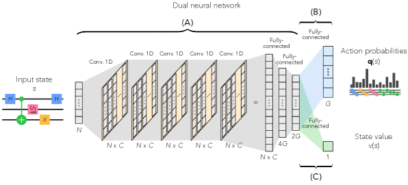
Appendix E Dual neural network

The dual neural network consists of convolution, policy prediction, and state-value prediction parts, respectively labeled as (A), (B), and (C) in Fig. A·4. The convolution part (A) is composed of 5 convolution and 2 fully-connected layers with Leaky ReLU activation functionsXu et al. (2015), the batch normalization techniqueIoffe and Szegedy (2015), and the dropout techniqueSrivastava et al. (2014). The input to the convolution part is an $N$ -dimensional vector representing a quantum circuit, and the output is $2G$ -dimensional vectors. The policy prediction part (B) is a fully-connected network with a softmax activation function. The input to the policy prediction part is a $2G$ -dimensional vector, and the output is a $G$ -dimensional vector ${\bf{q}}$ predicting a policy to search quantum circuits, where $G$ is the number of selectable quantum gates. The state-value prediction part (C) is a fully-connected network with a hyperbolic tangent activation function. The input to the policy prediction part is a $2G$ -dimensional vector, and the output is a scalar $v$ predicting a state value of the input quantum circuit. Please see Table A·I for more detailed parameters of the network. The network is trained by the adaptive moment estimationKingma and Ba (2014) with the beta hyperparameters of $(0.9,0.999)$ and the learning rate of 0.001.

References

Ladd et al. (2010) T. D. Ladd, F. Jelezko, R. Laflamme, Y. Nakamura, C. Monroe, and J. L. O’Brien, Nature 464, 45 (2010).
Alexeev et al. (2021) Y. Alexeev, D. Bacon, K. R. Brown, R. Calderbank, L. D. Carr, F. T. Chong, B. DeMarco, D. Englund, E. Farhi, B. Fefferman, et al., PRX Quantum 2, 017001 (2021).
Nielsen and Chuang (2010) M. A. Nielsen and I. L. Chuang, Quantum computation and quantum information, 10th ed. (Cambridge Univ. Press, Cambridge, 2010).
Montanaro (2016) A. Montanaro, npj Quant. Inform. 2, 1 (2016).
Preskill (2018) J. Preskill, Quantum 2, 79 (2018).
Córcoles et al. (2019) A. D. Córcoles, A. Kandala, A. Javadi-Abhari, D. T. McClure, A. W. Cross, K. Temme, P. D. Nation, M. Steffen, and J. M. Gambetta, Proc. IEEE 108, 1338 (2019).
Chow et al. (2012) J. M. Chow, J. M. Gambetta, A. D. Corcoles, S. T. Merkel, J. A. Smolin, C. Rigetti, S. Poletto, G. A. Keefe, M. B. Rothwell, J. R. Rozen, et al., Phys. Rev. Lett. 109, 060501 (2012).
Willsch et al. (2017) D. Willsch, M. Nocon, F. Jin, H. De Raedt, and K. Michielsen, Phys. Rev. A 96, 062302 (2017).
Gambetta et al. (2017) J. M. Gambetta, J. M. Chow, and M. Steffen, npj Quant. Inform. 3, 2 (2017).
Wendin (2017) G. Wendin, Rep. Prog. Phys. 80, 106001 (2017).
(11) IBM Quantum. https://quantum-computing.ibm.com/ (2021).
Kaelbling et al. (1996) L. P. Kaelbling, M. L. Littman, and A. W. Moore, J. Artif. Intel. Res. 4, 237 (1996).
Arulkumaran et al. (2017) K. Arulkumaran, M. P. Deisenroth, M. Brundage, and A. A. Bharath, IEEE Signal Process. Mag. 34, 26 (2017).
Silver et al. (2017a) D. Silver, J. Schrittwieser, K. Simonyan, I. Antonoglou, A. Huang, A. Guez, T. Hubert, L. Baker, M. Lai, A. Bolton, et al., Nature 550, 354 (2017a).
Silver et al. (2017b) D. Silver, T. Hubert, J. Schrittwieser, I. Antonoglou, M. Lai, A. Guez, M. Lanctot, L. Sifre, D. Kumaran, T. Graepel, et al., arXiv preprint arXiv:1712.01815 (2017b).
Peruzzo et al. (2014) A. Peruzzo, J. McClean, P. Shadbolt, M.-H. Yung, X.-Q. Zhou, P. J. Love, A. Aspuru-Guzik, and J. L. O’brien, Nat. Commun. 5, 4213 (2014).
Farhi et al. (2014) E. Farhi, J. Goldstone, and S. Gutmann, arXiv preprint arXiv:1411.4028 (2014).
Endo et al. (2021) S. Endo, Z. Cai, S. C. Benjamin, and X. Yuan, J. Phys. Soc. Jpn. 90, 032001 (2021).
Cerezo et al. (2021) M. Cerezo, A. Arrasmith, R. Babbush, S. C. Benjamin, S. Endo, K. Fujii, J. R. McClean, K. Mitarai, X. Yuan, L. Cincio, et al., Nat. Rev. Phys. 3, 625 (2021).
Nakaji et al. (2022) K. Nakaji, S. Uno, Y. Suzuki, R. Raymond, T. Onodera, T. Tanaka, H. Tezuka, N. Mitsuda, and N. Yamamoto, Phys. Rev. Res. 4, 023136 (2022).
Mitarai et al. (2018) K. Mitarai, M. Negoro, M. Kitagawa, and K. Fujii, Phys. Rev. A 98, 032309 (2018).
Fuchs and Van De Graaf (1999) C. A. Fuchs and J. Van De Graaf, IEEE Trans. Inform. Theory 45, 1216 (1999).
Khaneja et al. (2005) N. Khaneja, T. Reiss, C. Kehlet, T. Schulte-Herbrüggen, and S. J. Glaser, J. Mag. Res. 172, 296 (2005).
Khatri et al. (2019) S. Khatri, R. LaRose, A. Poremba, L. Cincio, A. T. Sornborger, and P. J. Coles, Quantum 3, 140 (2019).
Dalgaard et al. (2020) M. Dalgaard, F. Motzoi, J. J. Sørensen, and J. Sherson, npj Quant. Inform. 6, 6 (2020).
Peng et al. (2020) T. Peng, A. W. Harrow, M. Ozols, and X. Wu, Phys. Rev. Lett. 125, 150504 (2020).
Magann et al. (2021) A. B. Magann, C. Arenz, M. D. Grace, T.-S. Ho, R. L. Kosut, J. R. McClean, H. A. Rabitz, and M. Sarovar, PRX Quant. 2, 010101 (2021).
Fösel et al. (2021) T. Fösel, M. Y. Niu, F. Marquardt, and L. Li, arXiv preprint arXiv:2103.07585 (2021).
Moro et al. (2021) L. Moro, M. G. Paris, M. Restelli, and E. Prati, Commun. Phys. 4, 178 (2021).
Kimura et al. (2022) T. Kimura, K. Shiba, C.-C. Chen, M. Sogabe, K. Sakamoto, and T. Sogabe, J. Phys. Commun. 6, 075006 (2022).
Barenco et al. (1996) A. Barenco, A. Ekert, K.-A. Suominen, and P. Törmä, Phys. Rev. A 54, 139 (1996).
Nam et al. (2020) Y. Nam, Y. Su, and D. Maslov, npj Quant. Inform. 6, 26 (2020).
Ekert and Jozsa (1996) A. Ekert and R. Jozsa, Rev. Mod. Phys. 68, 733 (1996).
Aspuru-Guzik et al. (2005) A. Aspuru-Guzik, A. D. Dutoi, P. J. Love, and M. Head-Gordon, Science 309, 1704 (2005).
Xu et al. (2015) B. Xu, N. Wang, T. Chen, and M. Li, arXiv preprint arXiv:1505.00853 (2015).
Ioffe and Szegedy (2015) S. Ioffe and C. Szegedy, arXiv preprint arxiv:1502.03167 (2015).
Srivastava et al. (2014) N. Srivastava, G. Hinton, A. Krizhevsky, I. Sutskever, and R. Salakhutdinov, JMLR 15, 1929 (2014).
Kingma and Ba (2014) D. P. Kingma and J. Ba, arXiv preprint arXiv:1412.6980 (2014).

Table A·I: Architecture of the dual neural network

Part	Layer #	Layer	Hyperparameters
(A)	1	Convolution	output_channel=256, kernel_size=3, stride=1, padding=1
	2	Batch normalization	eps=1e-05, momentum=0.1, affine=True, track_running_stats=True
	3	Leaky ReLU	negative_slope=0.01
	4	Convolution	output_channel=256, kernel_size=3, stride=1, padding=1
	5	Batch normalization	eps=1e-05, momentum=0.1, affine=True, track_running_stats=True
	6	Leaky ReLU	negative_slope=0.01
	7	Convolution	output_channel=256, kernel_size=3, stride=1, padding=1
	8	Batch normalization	eps=1e-05, momentum=0.1, affine=True, track_running_stats=True
	9	Leaky ReLU	negative_slope=0.01
	10	Convolution	output_channel=256, kernel_size=3, stride=1, padding=1
	11	Batch normalization	eps=1e-05, momentum=0.1, affine=True, track_running_stats=True
	12	Leaky ReLU	negative_slope=0.01
	13	Convolution	output_channel=256, kernel_size=3, stride=1, padding=1
	14	Batch normalization	eps=1e-05, momentum=0.1, affine=True, track_running_stats=True
	15	Leaky ReLU	negative_slope=0.01
	16	Fully-connected	in_features=256× $G$ , out_features=4× $G$ , bias=True
	17	Batch normalization	eps=1e-05, momentum=0.1, affine=True, track_running_stats=True
	18	Leaky ReLU	negative_slope=0.01
	19	dropout	p=0.3
	20	Fully-connected	in_features=4× $G$ , out_features=2× $G$ , bias=True
	21	Batch normalization	eps=1e-05, momentum=0.1, affine=True, track_running_stats=True
	22	Leaky ReLU	negative_slope=0.01
	23	dropout	p=0.3
(B)	24-1	Fully-connected	in_features=2× $G$ , out_features= $G$ , bias=True
	25-1	Log softmax
(C)	24-2	Fully-connected	in_features=2× $G$ , out_features=1, bias=True
	25-2	tanh