Quantum circuits for exact unitary -designs and
applications to higher-order randomized benchmarking
Abstract
A unitary -design is a powerful tool in quantum information science and fundamental physics. Despite its usefulness, only approximate implementations were known for general . In this paper, we provide for the first time quantum circuits that generate exact unitary -designs for any on an arbitrary number of qubits. Our construction is inductive and is of practical use in small systems. We then introduce a -th order generalization of randomized benchmarking (-RB) as an application of exact -designs. We particularly study the -RB in detail and show that it reveals self-adjointness of quantum noise, a new metric related to the feasibility of quantum error correction (QEC). We numerically demonstrate that the -RB in one- and two-qubit systems is feasible, and experimentally characterize background noise of a superconducting qubit by the -RB. It is shown from the experiment that interactions with adjacent qubits induce the noise that may result in an obstacle toward a realization of QEC.
I Introduction
Randomness in quantum systems has been driving recent progress of quantum information science AE2007 ; D2005 ; DW2004 ; GPW2005 ; ADHW2009 ; DBWR2010 ; SDTR2013 ; HOW2005 ; HOW2007 ; AS2004 ; HLSW2004 ; S2005 ; BH2013 ; KRT2014 ; KL15 ; KZD2016 ; OAGKAL2016 ; B2018 ; G2019 ; BFNV2019 ; OSH2020 ; EAZ2005 ; KLRetc2008 ; MGE2011 ; MGE2012 ; B2018 ; PhysRevLett.112.240504 ; PhysRevA.93.012301 ; garion2020experimental ; PhysRevLett.122.200502 ; PhysRevA.87.030301 ; PhysRevLett.109.240504 ; PhysRevLett.109.080505 ; OWE2019 ; HROWE2020 as well as fundamental physics PSW2006 ; dRARDV2011 ; dRHRW2016 ; HP2007 ; SS2008 ; S2011 ; LSHOH2013 ; HQRY2016 ; RY2017 ; NWK2020 ; LFSLYYM2019 ; M2021 . Theoretically, quantum randomness is often formulated by a unitary drawn uniformly at random, also known as a Haar random unitary. However, the Haar randomness is physically unfeasible in large quantum systems. From the viewpoint of applications, the unitaries that have similar properties of a Haar random unitary are of great importance since they can be used instead of the Haar one. When a random unitary has the same -th order statistics as a Haar random unitary on average, it is called a unitary -design. For instance, when a protocol exploits the -th power of the measurement probability after applying a Haar random unitary on any state, the protocol also works even if the Haar random unitary is replaced with a unitary -design.
A unitary -design can be regarded as a quantum generalization of -wise independence AE2007 , and have many applications, ranging from communication D2005 ; DW2004 ; GPW2005 ; ADHW2009 ; DBWR2010 ; SDTR2013 ; HOW2005 ; HOW2007 , cryptography AS2004 ; HLSW2004 , algorithms S2005 ; BH2013 , sensing KRT2014 ; KL15 ; KZD2016 ; OAGKAL2016 , to potentially quantum supremacy B2018 ; G2019 ; BFNV2019 . A unitary -design is also related to another important concept in quantum information science, epsilon-net OSH2020 , implying more applications yet-to-be-discovered. Furthermore, the concept of unitary designs has opened a novel research field over quantum information science, quantum thermodynamics, strongly correlated physics, and quantum gravity PSW2006 ; dRARDV2011 ; dRHRW2016 ; HP2007 ; SS2008 ; S2011 ; LSHOH2013 ; HQRY2016 ; RY2017 ; NWK2020 . Experimentally, unitary designs and related methods have been exploited for benchmarking noisy quantum devices EAZ2005 ; KLRetc2008 ; MGE2011 ; MGE2012 ; B2018 ; PhysRevLett.112.240504 ; PhysRevA.93.012301 ; garion2020experimental ; PhysRevLett.122.200502 ; PhysRevA.87.030301 ; PhysRevLett.109.240504 ; PhysRevLett.109.080505 ; OWE2019 ; HROWE2020 , realizing quantum supremacy G2019 , demonstrating quantum chaos and quantum holography LFSLYYM2019 ; M2021 . It is also worthwhile to mention that unitary designs have been studied in combinatorial mathematics DGS1975 ; DGS1977 ; RS2009 ; R2010 ; RS2011 ; BNRT2020 . Hence, developing the theory of unitary designs is of substantial interest in a wide range of science, both theoretically and experimentally.
An important question about unitary -designs is how to implement them by quantum circuits. Many implementations of unitary -designs, both approximate and exact ones, were proposed DLT2002 ; BWV2008a ; WBV2008 ; GAE2007 ; TGJ2007 ; DCEL2009 ; HL2009 ; DJ2011 ; BWV2008a ; WBV2008 ; CLLW2015 ; NHMW2015-1 . In contrast, only approximate implementations of unitary -designs for general were known HL2009TPE ; BHH2016 ; NHKW2017 ; HM2018 ; HMHEGR2020 . Explicit constructions of exact unitary designs were left open except special cases RS2009 ; BNRT2020 ; BNZZ2019 . Approximate ones typically suffice in applications, but exact designs are more preferable in certain protocols especially when they are used multiple times in a single run of the protocol. If this is the case, the error from each approximate implementation accumulates and eventually spoils the protocol.
One of such protocols is a randomized benchmarking (RB) protocol EAZ2005 ; KLRetc2008 ; MGE2011 , a standard method for experimentally estimating quantum noise, where unitary -designs are used multiple times. Although the RB is experimentally-friendly and is widely used in various experimental systems, it reveals only the average gate fidelity. To obtain more information about the noise, a number of variants were proposed and experimentally implemented (see, e.g., Ref. HHFFW2019 and the references therein), which are all based on -designs. It is highly expected that, by using higher-designs, much more information about the noise in quantum systems can be extracted. To this end, explicit constructions of exact unitary -designs are important.
Constructing exact designs is, however, by far non-trivial. The difficulty is illustrated by a spherical -design, a random real unit vector analogous to a unitary -design. The existence of exact spherical -designs was proven in a non-constructive manner more than three decades ago SZ1984 . Since then, more concise proofs and explicit constructions have been under intense investigation in combinatorial mathematics (see e.g., Refs. RB1991 ; WV1991 ; BB2009 ; BRV2013 ; CXX2019 and the references therein). In particular, it was only recently that constructions in general cases X2020 and explicit constructions, in the sense that all the algorithms are given in a computable form BNOZ2020 , were proposed. Finding explicit constructions of exact unitary designs, since they are more complicated than spherical designs, is a rather non-trivial problem.
In this paper, we provide for the first time an explicit quantum circuit that generates an exact unitary -design for any on the arbitrary number of qubits. More specifically, we show that an exact unitary -design on -dimensional Hilbert space, i.e., qudit, can be generated from those on smaller spaces, which is obtained based on the recent mathematical results by some of the authors BNOZ2020 . Using this result, we provide an inductive construction of quantum circuits for exact unitary -designs on qubits: we first construct a unitary -design on a single qubit and then extend it to qubits. Unfortunately, the circuit fails to be efficient, but is still of practical use when the size of the system is small.
As an application of exact unitary designs, we introduce the -th order RB, or the -RB for short, that harnesses the power of exact unitary -designs. The standard RB corresponds to the -RB. The -RB enables us to experimentally characterize the higher order properties of quantum noises in the manner free from state-preparation and measurement (SPAM) errors. We especially investigate the -RB in detail and show that it reveals self-adjointness of the noise in the system. The self-adjointness is a new metric of the noise related to the feasibility of quantum error correction (QEC): small self-adjointness implies that the noise cannot be approximated by any stochastic Pauli noise. The noise on the system being stochastic Pauli is desirable both in theory and in practice. Stochastic Pauli noises are the commonly-used noise models in theoretical studies of QEC, since they are easy to numerically handle, and the properties of QEC, such as error thresholds and logical error rates, for stochastic Pauli noises are well-understood. Also, there is a practical advantage if the noise on the system is stochastic Pauli since they can be corrected simply by applying Pauli operators, making the error correcting scheme easier in general.
After numerically demonstrating the feasibility of the -RB, we perform the -RB in a superconducting system and estimate the self-adjointness of background noise, showing that the -RB experiments are feasible. From the experiment, we find that the interactions with adjacent qubits especially decrease the self-adjointness, which may lead to degradation of the performance of QEC with standard decoders. Hence, either improving the system or extending the noise model in theoretical studies of QEC, or both, is important for further experimental developments of quantum information technology.
This paper is organized as follows. In Sec. II, we provide a general introduction of unitary -designs. Our main results are summarized in Sec. III for the quantum-circuit construction of exact unitary -designs, and in Sec. IV for the -RB protocols. A summary of the experiment of the -RB is provided in Sec. V. After we explain the structure of the remaining paper in Sec. VI, we provide a proof of the explicit construction in Sec. VII and the theory of the -RB in Sec. VIII. The details of the experiment are provided in Sec. IX. We conclude our paper with summary and discussions in Sec. X. Technical statements are provided in Appendices.
II Unitary -designs
Let be the unitary group of degree . The Haar measure on is the unique unitarily invariant measure on the unitary group, i.e., it satisfies
| (1) |
When it is needed to clarify the degree of the unitary group, we denote the Haar measure by .
A unitary -design is defined by a finite set of unitaries that mimics the -th order statistical moment of the Haar measure . Amongst several equivalent definitions L2010 , we here adopt the following definition.
Definition 1 (Unitary -design).
For , a finite set of unitaries is a unitary -design if
| (2) |
where is a uniform average over , and is the average over the Haar measure.
From an operational viewpoint, this definition implies that a unitary -design cannot be distinguished from a Haar random unitary on average even when copies of the unitary are given. To clasify this, let us define a quantum operation, i.e., a completely-positive and trace-preserving (CPTP) map, by
| (3) |
for any quantum state on qudits, where is either the Haar measure on a qudit or a uniform measure over a unitary -design . Then, we can show that Definition 1 is equivalent to that (see e.g. L2010 )
| (4) |
This implies that, in any experiments that use copies of a random unitary, no difference will be observed on average when a -design is used instead of the Haar one.
For instance, let us consider the probability distribution when a one-qudit state is measured by a given POVM after the application of a unitary . By setting the -qudit state in Eq. (3) to and using Eq. (4), it follows that, for any ,
| (5) |
Thus, the distribution of the measurement outcomes for a Haar random unitary and that for an unitary -design exactly coincide up to the -th order on average. Note that this is merely an example, and Eq. (4) implies much more: a Haar random unitary cannot be differentiated from a unitary -design even by more complicated experiments over qudits.
The existence of an exact unitary -design on for any and follows from the Carathéodoty’s theorem and the fact that the dimension of the space, on which is defined, is finite. Note however that the proof indicates only the existence of an exact unitary -design. How to explicitly construct an exact unitary -design has been a highly non-trivial problem.
In our construction, it is convenient to introduce a strong unitary -design.
Definition 2 (Strong unitary -design).
For , a finite set of unitaries on is called a strong unitary -design if
| (6) |
for and .
Clearly, a strong unitary -design is a unitary -design. Unlike standard unitary designs, strong unitary designs do not have a clear operational interpretation in quantum information processing, but we use it in the intermediate step of our construction.
III Main result 1 – quantum circuits for exact unitary designs –
In this section, we provide explicit constructions of strong unitary -designs for any . In particular, a quantum circuit for a strong unitary -design on qubits is provided. We start with preliminaries in Subsec. III.1, and provide the construction in Subsec. III.2. We then comment on the circuit complexity of the construction in Subsec. III.3.
III.1 Preliminaries
Unitary designs have been studied in terms of representation theory RS2009 ; RS2011 since the operator in the definition can be regarded as a representation of the unitary group. Our construction is based on representation theory, where irreducible decomposition of the operator plays an important role. A brief introduction of irreducible representations (irreps) will be provided in Section VII.1. Here, we mention a couple of well-known facts that are necessary to state our main result.
Any irrep of the unitary group can be indexed by a non-increasing integer sequence of length , i.e., for , and B2004 . In particular, spherical representations of with respect to are of great importance in the construction. Let be a set of all non-increasing integer sequences in the form of
| (7) |
where and . The spherical representation is the irrep indexed by GW2009 . For a spherical representation , a zonal spherical function is defined by the unique bi--invariant function JC1974 ; R2010 ; BNOZ2020 . The zonal spherical functions are a certain type of symmetric polynomials, and can be explicitly written down (see, e.g., Appendix A of Ref. BNOZ2020 ).
III.2 Inductive constructions
Our main technical result is to construct a strong unitary -design on from those on and on .
Theorem 3.
Let be a positive integer such that . Define a set of unitaries in by
| (8) |
where and are strong unitary -designs on and , respectively. Let be such that
| (9) |
where is the zonal spherical function for . Let be a unitary defined by
| (10) |
where and , and is the identity matrix of size . Then,
| (11) |
is a strong unitary -design on .
Theorem 3 follows from a more general result BNOZ2020 shown by some of the authors, which works not only for the unitary group but also for a broader class of compact groups. For the sake of completeness, we provide a direct proof of Theorem 3 in Sec. VII.
We then claim that
| (12) |
where is the -th root of unity, is a strong unitary -design on for any . This is easily checked by direct calculations:
| (13) | |||
| (14) |
where is the Kronecker delta. Hence, we have for , implying that is a strong unitary -design.
From Theorem 3 and , a strong unitary -design on a qudit can be inductively constructed.
Corollary 4.
For , let be a set of unitaries given by
| (15) |
where with being the -th root of unity, and be such that
| (16) |
Using a unitary , where is the Pauli- operator, we obtain that
| (17) |
is a strong unitary -design on a qudit.
In this construction, it is important to obtain zeros for the zonal spherical functions . This is computationally feasible since they are polynomials of one variable and are explicitly given (see Appendix A of Ref. BNOZ2020 ). Furthermore, contains only elements. Hence, we need to solve polynomials with one variable, which is tractable as far as is not too large.
We now consider a strong unitary -design on qubits. Again using Theorem 3, we obtain the quantum circuit on qubits based on that on qubits. See also Fig. 1.
Corollary 5.
Let be a strong unitary -design on qubits, and be a set of controlled-unitaries on qubits, defined by
| (18) |
For , where , let be such that
| (19) |
Representing in binary form such as , we write as . Let be a single-qubit -rotation controlled by qubits, defined by
| (20) |
Then,
| (21) |
is a strong unitary -design on qubits.
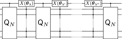
Corollary 5 implies that a quantum circuit for an exact unitary -design can be inductively constructed from a strong unitary -design on one qubit, i.e., that on . Furthermore, a strong unitary -design on can be constructed using Corollary 4. Thus, combining Corollaries 4 and 5, we obtain a quantum circuit for an exact unitary -design for any and on an arbitrary number of qubits.
Note that the circuit, constructed in this way, can be explicitly decomposed into two-qubit gates. The controlled unitary part contains up to three-qubit gates, if the circuit on qubit is already decomposed into two-qubit gates. The three-qubit gates can be easily rewritten as a series of two-qubit gates. Also, the -rotation controlled by qubits, , can be decomposed into a sequence of two-qubit gates of polynomial length using sufficiently many number of ancillary qubits, which is based on a classical oracle that computes the angle from (see Appendix A).
In special cases, we can find a much more concise construction based on a similar technique.
Proposition 6.
Let be the Clifford group on qubits. There exists a fixed two-qubit unitary , such that is an exact unitary -design on qubits.
Analytically, we can prove that there exist unitaries and such that is an exact unitary -design on qubits BNOZ2020 . Also, an algorithm for computing the unitaries and is given. It, however, turns out from numerics that it is not necessary to apply two extra unitaries if we choose a proper unitary , which leads to Proposition 6. An explicit form of the unitary is numerically obtained and is provided in Appendix B. Note that the existence of is confirmed numerically, so the statement holds up to the numerical precision.
This construction is only for a -design on qubits, but the number of unitaries in the -design is much smaller than that of Corollary 5. It is an open problem whether a similar construction works for higher-designs on a larger number of qubits.
III.3 Efficiency and comparison with a Haar unitary
To quantitatively evaluate the complexity of the quantum circuit for an exact unitary -design obtained in Corollary 5, we provide an order estimate of the number of two-qubit gates in the circuit. Assuming and using the fact that due to the Hardy and Ramanujan formula for the asymptotics of the number of partitions, we obtain
| (22) |
to the leading order of . Hence, it is necessary to use exponentially many two-qubit gates as the number of qubits increases. This inefficiency of the quantum circuit may be intrinsic since the construction is inductive.
There is another source of inefficiency. In Corollary 5, it is necessary to find zeros of zonal spherical functions (see Eq. (19)) for all . The zonal spherical function is given in terms of the summation of the (normalized) Schur polynomials (see Appendix A in Ref. BNOZ2020 ). It is unlikely that the Schur polynomials have polynomial size algebraic formulas in general SchurPoly2019 . Moreover, the number of variables for each is . Hence, finding zeros of zonal spherical functions is computationally intractable.
In total, the construction for an exact unitary -design on a large number of qubits is inefficient from both quantum-circuit and classical-computation viewpoints. We, however, think that our construction and our proof technique will form a solid basis of searching more efficient constructions of exact, as well as approximate, unitary designs. We also emphasize that, despite its inefficiency, our construction is of practical use on a few-qubit system, as we seek in the following sections.
Before we conclude this section, we comment on advantages of our construction of an exact unitary -design over a direct implementation of a Haar random unitary. A naive way of implementing a Haar random unitary by a quantum circuit consists of three steps. First, we sample a Haar random unitary as a matrix by a classical computer. A classical algorithm for this is known M2007 , but it is trivially inefficient since the size of the matrix is exponentially large. We then classically compute a decomposition of the unitary matrix into a sequence of two-qubit unitaries, providing a classical description of a quantum circuit for the unitary. This step is also inefficient, and the resulting quantum circuit is almost surely composed of the exponentially many number of two-qubit gates. Finally, we implement the circuit in practice.
This quantum circuit for a Haar random unitary is inefficient in terms of the number of qubits, and so, cannot be of practical use in a large system. Even in a small system, this naive implementation has a crucial difficulty that, every time a unitary is sampled, the above protocol outputs a quantum circuit with a rather different sequence of various two-qubit gates. This implies that, in each sampling, one needs to significantly modify the quantum circuit. This is in a sharp contrast to our quantum circuit for a unitary -design based on Corollary 5 since it has a fixed structure. In each sampling, only what one needs to do is to randomly choose single-qubit gates, or more precisely elements of from (see Eq. (12)), and to plug them into the quantum circuit with a fixed structure. This will help practical implementations of the circuit in small systems.
It should be also noted that the single-qubit gates in our construction can be sampled from a discrete set, though sampling from a continuous gate set is necessary in the direct implementation of a Haar random unitary. This is another advantage of our construction.
IV Main result 2 – Higher-Order Randomized Benchmarking –
We here introduce a higher-order generalization of the standard RB that uses exact unitary -designs. We call it the -th order RB, or simply -RB. The standard RB corresponds to -RB. From the higher-order RB, more information about the noise can be extracted. In particular, we show that a new characterization of the noise, which we call self-adjointness, can be estimated from the -RB.
Before we proceed, we emphasize that exact unitary designs, not approximate ones, are of crucial importance in the RB-type protocols. This is because the protocol uses unitary designs multiple times. Hence, if each unitary has an error due to the approximation, it accumulates in the whole process and results in a large error at the end.
Since the goal of the RB-type protocol is typically very high, such as benchmarking the fidelity , the error originated from the approximate designs would spoil the protocol. Hence, the use of exact unitary designs is of key importance. This point is more elaborated on in Subsec. IV.4.
In Subsec. IV.1, we overview a couple of metrics of the noise, i.e., the average fidelity and unitarity, and introduce the self-adjointness. The importance of the self-adjointness in QEC is argued in Subsec. IV.2. We then introduce the -RB in Subsec. IV.3. We argue the importance of exact designs in more detail in Subsec. IV.4. We focus on the -RB in Subsec. IV.5 and show that the self-adjointness and the unitarity of the noise can be estimated from the -RB at the same time. We briefly comment on the scalability of the -RB in Subsec. IV.6.
IV.1 Characterizing noises
A noise acting on a -qubit system is formulated by a completely-positive and trace-preserving (CPTP) map. Let be defined as . The average fidelity and the unitarity are defined by
| (23) | |||
| (24) |
respectively, where , and is the Schatten 2-norm. The average fidelity satisfies , and if and only if the system is noiseless, i.e., is the identity channel, while the unitarity satisfies , and if and only if the noise is coherent, i.e., is a unitary channel. The unitarity is an important metric in the context of QEC since coherent noise is known to be hard to correct in general KLDF2016 ; SWS2015 ; SFK2017 .
In the RB-type protocols, it is more natural to use a fidelity parameter rather than the average fidelity itself. It is defined by
| (25) |
and satisfies .
We next introduce a self-adjointness of the noise. For any linear map , an adjoint map is defined by . A noise is called self-adjoint if , which is equivalent to that all the Kraus operators of are self-adjoint.
The self-adjointness of the noise is defined by
| (26) |
The normalization constant is chosen such that . Obviously, if and only if is self-adjoint, i.e. . Note that the self-adjointness has two contributions from the noisy map , one is from the unital part and the other from the non-unital part. The non-unital part of the noise makes the self-adjointness less than one since, if is not unital, then is not trace-preserving, which implies that .
To clearly separate the two contributions, we introduce a self-adjointness parameter . Using , we defined it by
| (27) |
The self-adjointness parameter is related to the self-adjointness and the unitarity by
| (28) |
where is a measure of the non-unital part of the noise (see Subsec. VIII.1 for the definition). We can clearly observe that consists of two factors, the unital part and the non-unital part .
The three metrics of noises, namely, fidelity, unitarity, and self-adjointness, all capture different properties of the noises. The fidelity reveals the first order property of the noises, while the unitarity and the self-adjointness, which are independent to each other, reveal the second-order. In order to improve noisy quantum devices, it is of crucial importance to obtain the information of noise as much as possible. Hence, it is certainly of practical use to introduce the self-adjointness as a new metric of noise. In addition, we argue in the next subsection that the self-adjointness has important implications for QEC.
IV.2 Importance of self-adjointness in QEC
The most important family of self-adjoint noises is stochastic Pauli noises, whose Kraus operators are all proportional to Pauli matrices. In QEC, Pauli noises are the standard yet most important class of noises both in theory and in practice. From a theoretical perspective, Pauli noises are easy to numerically handle. Hence, most numerical calculations have been carried out by assuming Pauli noises, and it has been confirmed that QEC has preferable features, such as exponential decreases and threshold behaviors of logical error rates, if the noise is Pauli.
The noise being Pauli is also practically preferable in experimental realizations of QEC since it typically simplifies the decoding tasks. This is especially the case for stabilizer codes, such as surface and color codes, whose standard decoders are to estimate what types of Pauli operators should be applied on which physical qubits during recovery operations. For stochastic Pauli noises, if the estimation goes well, the state is fully retrieved with high probability by applying Pauli operators to the suitable physical qubits. In contrast, it is not possible to fully correct non-Pauli noises by applying Pauli operators since they generate undesired coherence between different code spaces. Thus, QEC of non-Pauli noises generally suffers from degradation of logical error rates when the standard decoders are used SFK2017 ; BEKP2018 or requires more complicated algorithms for retrieving the performance of QEC. Neither of them is preferable in practice since it induces additional experimental difficulties.
For these reasons, it is desirable to check that the noise on an experimental system is stochastic Pauli. To this end, the self-adjointness provides useful information since, if , then the noise is far from self-adjoint and cannot be approximated by Pauli noises. This implies that the practical situation differs from the standard assumption in theoretical studies of QEC and incurs additional difficulties on decoding procedure. Thus, the self-adjointness provides practical information about the feasibility of QEC using Pauli-based decoders.
Note that the difficulty of QEC for non-Pauli noises, captured by the self-adjointness, highly depends on the assumptions in quantum error correction schemes. When any decoding procedure is available, it would not be so important whether the noise is Pauli or non-Pauli. When this is the case, the unitarity will be a more suitable metric of noise relevant to the feasibility of QEC KLDF2016 ; SWS2015 ; SFK2017 . Note also that non-Pauli noises can be always transformed to a Pauli noise by Pauli-twirling. However, Pauli-twirling induces additional noise onto the system and, as a result, the performance of QEC will degrade. Thus, it is practically desirable to manufacture the system so that the noise is stochastic Pauli.
We also provide a pedagogical example of noise, where performance of QEC can be directly captured by the self-adjointness but not by fidelity nor unitarity. Consider a -rotation error around the -axis on one qubit, i.e., , where is the Pauli- operator. The average fidelity and the self-adjointness can be obtained as
| (29) | ||||
| (30) |
The unitarity is for any .
One may expect that the -rotation error is easier to correct than the -rotation since the former has higher fidelity than the latter. However, this is not the case since -rotation is simply a perfect bit-flip that can be trivially corrected, while the -rotation error is known to be particularly hard to correct DP2017 . Thus, neither the average fidelity nor the unitarity, which is for both errors, is a good metric of the error correctability. In contrast, the self-adjointness clearly captures whether the error can be corrected, at least in this case, since and are the minimum and the maximum values of the self-adjointness, respectively.
IV.3 General description of the -th order RB
We now introduce the -RB using an exact unitary -design . As is the case for the standard RB, we assume that the noise is gate- and time-independent, so that the noisy implementation of is given by , where is the CPTP map that represents the noise, and we used the notation that .
Let and be the initial and measurement operators, respectively, which we assume to be Hermitian. We first apply a sequence of unitaries onto the initial operator . Each is chosen uniformly at random from , which we denote by . We then apply its inverse , and measure .
If the system is noiseless, , this protocol results in a trivial expectation value that
| (31) |
due to the inverse unitary . However, when the system is noisy, the expectation value becomes
| (32) |
which in general differs from . The basic idea of the RB-type protocol is to extract some information about the noise from the difference.
In the -RB, we especially focus on the average of the -th power of the expectation value over all choices of the unitary sequence. That is,
| (33) |
Using the representation-theoretic technique, it can be shown that is generally given in the following form:
| (34) |
where labels the irreps of the unitary group, and are matrices with being the multiplicity of the irrep . This is well-known in the literature of RB-type protocols, but we provide a proof in Sec. VIII.3 for completeness.
Despite its abstract expression, Eq. (34) has an important implication that the matrix depends only on and , but not on and . Hence, from the experimental data of for various , it is in principle possible to estimate the matrix , which contains certain information of the noise , in the way independent of and .
In practice, the most important situation is when the representation is multiplicity-free, i.e., for any . In this case, reduces to a much simpler form:
| (35) |
where . Note that since is a bounded function. Hence, in this case, becomes a sum of some exponentially decreasing functions with respect to .
To be more concrete, let us recall the standard RB, corresponding to the -RB. As shown in Ref. EAZ2005 , is given by
| (36) |
where and depend only on and , and is the fidelity parameter of the noise . Thus, by fitting experimentally obtained data of for different with the fitting function , we can estimate the fidelity parameter .
IV.4 Importance of exact designs in RB
In the RB protocol, it is important to use exact unitary designs because designs are used many times, sometimes a few hundreds to a thousand, in a single run of the protocol. To illustrate this, let us consider the -RB when the unitary -design in the protocol is -approximate.
Let be the length of the unitary sequence as above. It is straightforward to show that,
| (37) |
where ’s are some constants that depend on , , , and how the design differs from the exact one. See Subsec. VIII.4 for the derivation. Compared to the -RB with exact ones, i.e., Eq. (36), fitting this function with respect to is much harder since it is not a simple exponential decay.
The fitting may go well if . This requires a very high precision of the design since can be a few hundreds in actual experiments. For instance, when , the degree of approximation of the unitary design should be order or so. Although it is possible to achieve this degree of approximation by a sufficiently long quantum circuit BHH2016 ; NHKW2017 ; HMHEGR2020 , the RB becomes unpractical if we use such a long circuit at every use of a unitary design in the protocol and repeat it a few hundreds times.
There might be a possibility to improve Eq. (37) by using different constructions of approximate unitary designs at every step, by which the differences from the exact design may become random so that they cancel out in total. This will be an interesting question, but at this point, it is not clear if such a technique works. Also, even if it works, we need to assume additional structures of approximate constructions.
The higher-order RB with approximate designs will incur more difficulty in practice. Since it uses higher moment of the outcomes, the fitting function becomes more complicated than Eq. (37) when one uses approximate designs. Similarly to the -RB with approximate -designs, much better degree of approximation, that is, longer quantum circuits, will be needed, which is not practical. Thus, we conclude that exact unitary designs are of crucial importance in a practical implementation of the -RB.
IV.5 Second-order RB
We next focus on the -RB using exact unitary -designs, and show that the -RB reveals the self-adjointness of the noise. To this end, we set the initial operator to a traceless one, i.e., . This setting, together with the fact that the noise is trace-preserving, makes the representation multiplicity-free (see Appendix C). Hence, the expectation value for the -RB is given by a sum of exponentially decaying functions as shown in Eq. (35).
Note that the expectation value for a traceless initial operator can be obtained by performing the same experiment for two different quantum states and , and by taking the difference of the expectation values before they are squared. That is,
| (38) |
where is a traceless operator.
Our second main result in this paper is about as summarized in Theorem 7.
Theorem 7.
In the above setting, is given as follows. For single-qubit systems,
| (39) |
where , and are the fidelity parameter, the unitarity, and the self-adjointness parameter of the noise , respectively. For multi-qubit systems,
| (40) |
where depend only on the noise . Moreover, they satisfy
| (41) |
where
| (42) | |||
| (43) | |||
| (44) |
See Subsec. VIII.5 for the proof.
In the single-qubit case, is a sum of two exponentially decaying functions with respect to . Hence, from the double-exponential fitting of the experimental data of , we can simultaneously estimate and . Since it can be shown that the former is not less than the latter, we can estimate which of the two decaying rates corresponds to which quantity without any ambiguity. It is also possible to estimate the fidelity parameter from the same data set by computing because a unitary -design is also a unitary -design. Thus, from the experiment of the -RB on a single qubit, all of , and can be estimated simultaneously.
In multi-qubit systems, has a little more complicated form and consists of four exponentially decaying functions. Also, the decaying rates do not directly correspond to neither the unitarity nor the self-adjointness parameter. We observe from Eq. (41) that can be obtained from a linear combination of the decaying rates , the value of , and .
One may think that, in the case of multiple qubits, it is practically intractable to accurately fit four exponentially decaying functions from experimental data because each data point has an error. This difficulty can be circumvented by choosing appropriate initial and measurement operators. By doing so, we can set some of zero in the ideal situation (see Tab. 1). This allows us to estimate the decaying rates one by one. Note that the initial and measurement operators in Tab. 1 are all diagonal in the computational basis. Hence, it suffices to perform the experiments for the four initial operators , and , with the measurement in the computational basis. From the data of these experiments, it is possible to reproduce all cases listed in Tab. 1 by post-processing.
In the multi-qubit case, the ambiguity remains to decide which of the decaying rates corresponds to which quantity. This is the case even when we use the above step-by-step estimation of the rates since, for instance, it is not clear if the unitarity is larger or smaller than . In this case, we need to additionally perform the unitarity benchmarking WGHF2015 ; HHFFW2019 to separately estimate . If we have an estimated value of , the step-by-step estimation allows us to decide all decaying rates without any ambiguity.
| 16/15 | 4/15 | ||
| 48/5 | 41/15 | ||
| 16/3 | 1/3 | ||
| 0 | 2/3 |
IV.6 Scalability
The -RB for inherits most of the desired properties of the RB-type protocols. For instance, it is experimentally-friendly since, apart from using higher-designs, the difference of the -RB from the standard RB (-RB) is only taking the -th power of the expectation value before the average. It is also true that the -RB is free from SPAM errors (see Eqs. (34) and (35)).
The property that the standard RB does have and the -RB does not in general is the scarability. This is for two reasons. First, no efficient construction of exact unitary -designs is known for so far. Second, in the -RB protocol, it is necessary to apply the inverse unitary at the end of the unitary sequence. Hence, we need to beforehand compute the inverse of each sequence. When the system is large, the task is intractable in general. This difficulty is avoided in the standard RB by using the Clifford group, which is an exact unitary -design. Since the inverse is contained in the group, we can find the inverse relatively easily. One may expect that the difficulty of finding the inverse could be also avoided in the -RB by using the -design that is also a group, which is called a unitary -group BNRT2020 . However, it is known that unitary -groups do not exist for if the number of qubits . Thus, in the -RB for , the hardness of finding the inverse in a large system is inevitable.
Nonetheless, we emphasize that, in the current experimental situations, the RB-type protocols for more than three qubits are practically intractable due to the limitation of the coherent time. Thus, the experimental use of the RB-type protocols is currently aiming to characterize the noise on one- or two-qubit systems in a concise manner. Considering this fact, even if the -RB is not scalable, it is practically useful and beneficial: it is as concise as the standard RB and provides more information about the noise, such as self-adjointness.
V Main result 3 – -RB in a superconducting system –
We finally implement the -RB in a superconducting system and estimate the self-adjointness of background noise. Unlike the analytical studies, the expectation values and the average over a unitary -design cannot be taken with arbitrary precision in experiments since the number of repetitions of experiment is practically limited. To check that this limitation does not cause any problem in the evaluation of the self-adjointness, we start with numerically investigating the feasibility of the -RB in Subsec. V.1. We then provide a summary of experimental results in Subsec. V.2.
In recent years, a number of experiments have been performed to characterize various noises on superconducting quantum systems in detail Wilen2021 ; HAN202110 ; McEwen2021 ; mcewen2021resolving . From our experiments, we show that the interactions with the adjacent qubits particularly decrease the self-adjoinenss and may cause problems toward realizations of QEC. In particular, our result implies that there exists a gap between the superconducting system and the common noise model used in theoretical studies of QEC, and also that the standard decoders of stabilizer codes may suffer from degradation of logical errors. Hence, toward the realization of QEC, it is desired to further improve the system or to develop the theory of QEC.
V.1 Numerical evaluation
When the -RB is practically implemented, there are two additional concerns. One is originated from the fact that the expectation value is obtained from a limited number of measurements in the basis of , resulting in an error due to a finite number of measurements. The other originates from the evaluation of the average over the sequence of unitaries in the -design. Ideally, all sequences in should be taken, but practically, the average is often evaluated from a small subset in of randomly chosen sequences, leading to an additional error of estimation.
Taking sufficiently many measurements and samplings of unitary sequences will reproduce the analytical results with high accuracy. However, it is complicated to analytically derive the numbers sufficient for achieving a desired accuracy. We hence perform numerical experiments and show that experimentally-tractable numbers of samplings are sufficient for a reliable -RB.
V.1.1 One-qubit cases
In the case of single-qubit systems, we consider a specific noisy map given by
| (45) |
which is characterized by three parameters . The first term of the right-hand side represents a unitary part and the second term represents a stochastic part of the noise. A parameter determines a ratio between them. Hence, we can consider as a coherent parameter of noise, e.g., noise is unitary when and is a probabilistic Pauli noise when . The parameters and represent the rotation angle of the unitary part and the error probability of the stochastic part, respectively. For simplicity, we choose such that the fidelity parameters of unitary and stochastic parts are equal, that is, . Then, the fidelity parameter becomes independent of the coherent parameter .
To perform the -RB for this noise, we may use the exact -design constructed in Corollary 5. However, it is known that the icosahedral group, which we denote by , forms an exact -design on one qubit RS2009 . Since the icosahedral group has less cardinality than our inductive construction, we use it in the following analysis.
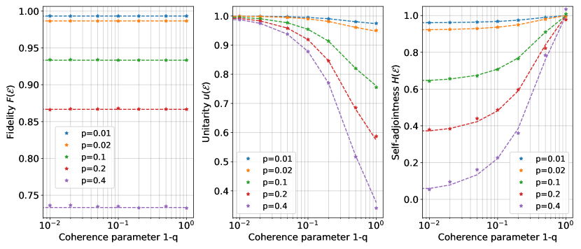
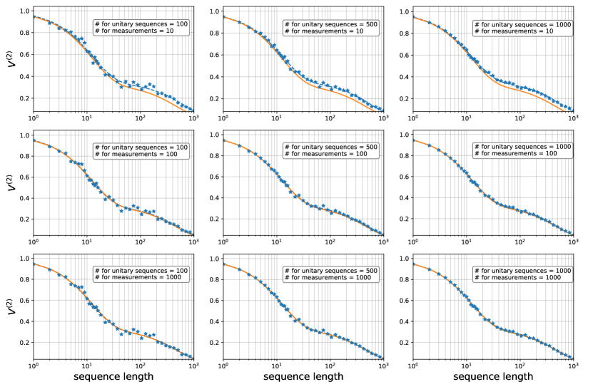
The numerical results for the -RB on a single qubit are shown in Fig. 2. For each sequence length , we have taken random unitary sequences from and have had measurements to obtain a single data point of . A detailed fitting procedure is provided in Subsec. IX.1.
To check the accuracy of the -RB, we consider the relative errors , where and are the theoretical value and the fitting value, respectively. Note that for all the fitting values when a fidelity close to unity is achieved. For almost all data points of and , we find that the relative errors are less than , except the case when is large, or equivalently, when the fidelity is small. The relative error becomes moderately large, such as , when and , corresponding to . This is because the decaying rate of the second term in Eq. (39) is rather small, making the fitting difficult. However, such a case is not practically relevant since the fidelity is typically . Thus, we conclude that the 2-RB on 1-qubit systems works well in practice.
To analyze the dependence of the accuracy of the -RB on the number of measurements and samplings of random unitary sequences, we additionally perform the 2-RB on one qubit with the various numbers of measurements and samplings. The results are summarized in Tab. 2, where we set the noise parameters to and . From these results, it appears that setting the numbers of measurements and samplings of random sequences to a few hundreds is sufficient for a good estimate. These results further indicate that increasing the number of random sequences rather than the number of measurements is preferable to improve the accuracy. See Subsec. IX.1 for the details.
| # of meas. | # of sequences | |||
|---|---|---|---|---|
| 10 | 100 | |||
| 10 | 500 | 0.986(1) | 0.9984(1) | 0.93(1) |
| 10 | 1000 | 0.986(6) | 0.9984(3) | 0.92(3) |
| 100 | 100 | 0.986(3) | 0.9980(8) | 0.92(2) |
| 100 | 500 | 0.986(5) | 0.9980(4) | 0.92(3) |
| 100 | 1000 | 0.986(6) | 0.9979(4) | 0.92(1) |
| 1000 | 100 | 0.986(3) | 0.9980(1) | 0.92(3) |
| 1000 | 500 | 0.986(4) | 0.9979(5) | 0.92(3) |
| 1000 | 1000 | 0.986(6) | 0.9978(9) | 0.92(2) |
| 0.9866 | 0.99793 | 0.9247 |
V.1.2 Two-qubit cases
For two-qubit systems, we consider the noise given by
| (46) |
which is similar to the one-qubit case. We choose as , so that is independent of the coherent parameter . In this case, we use the construction of exact unitary -designs given in Proposition 6.
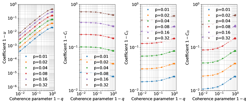
In the two-qubit case, it is needed to fit the experimental data by a sum of four exponentially decaying functions, which is in general not easy especially when each data point has errors caused by the finite number of measurements and samplings of unitary sequences. To avoid this difficulty, we use the method explained in Subsec. IV.5, and determine the four decaying rates, i.e., , and in Eq. (40), one by one.
The results are shown in Fig. 3. We have taken random unitary sequences for each sequence length and the parameters . A detailed process of fittings are explained step by step in Sec. IX.1. In the figure, fitted values are shown as data points. Dashed lines are drawn with theoretically calculated values.
Similarly to the case of the single-qubit -RB, we have checked the relative errors of the fitting results to the theoretical values. The errors are all below for all the points except the case when the theoretical value is exactly zero. As in the case of single-qubit 2-RB, when we calculate and from the fitting values, the relative values of almost all the data points are less than . While the relative errors become large when , such a case is not a problem in typical calibration scenario. Thus, the -RB works in actual situations also in the case of two-qubit systems.
V.2 Experimental implementations of the 2-RB
We demonstrate the -RB in a superconducting-qubit system. We first explain the setup of our experiments, and then verify the feasibility of the -RB experiment by comparing the unitarity obtained from the -RB with that from the unitarity benchmarking (UB) WGHF2015 ; HHFFW2019 . We finally characterize background noise of the system. As the background noise is gate- and time-independent, it satisfies the assumptions of the -RB (see Subsec. IX.2 for the detail).
V.2.1 Experimental setup
We use two superconducting qubits ( and ) coupled with each other via an electric dipole interaction, which are a part of our -qubit device tamate2021scalable . In all the experiments below, we use the qubit as a target qubit of the single-qubit -RB and, in some experiments, as an environmental qubit that induces additional error onto .
The simplified system Hamiltonian is formulated as follows,
| (47) |
where is the eigenfrequency of the -th qubit and is an effective interaction strength between the qubits gambetta2006qubit . It can be interpreted that the eigenfrequency of switches depending on the quantum state of . When is in the () state, has the eigenfrequency (). In the Bloch sphere representation, the state vector of the qubit rotates around the -axis with its eigenfrequency as the angular velocity.
We use a local oscillator synchronized with the eigenfrequency of the qubit for observation. The state vector is stationary in a rotating frame of the local oscillator since the -axis rotation speed of the Bloch vector matches with that of the measurement basis. The rotation frame picture also holds when the qubit couples to the adjacent qubit when the qubit is in the or state. For instance, when the qubit is always in the state, the eigenfrequency of is . We can detune the frequency of the local oscillator from the qubit frequency by to make the state vector of stationary.
It is, however, impossible to keep track of the eigenfrequency of the qubit when the state of the adjacent qubit varies. This results in an inevitable -rotation occurring in the quantum state. In an actual experiment involving multiple qubits, the frequency of the local oscillator is usually set to to minimize the average -rotation angle. See Subsec. IX.2 for the detail.
V.2.2 Comparison with the UB
| Experiment | Group | |||
|---|---|---|---|---|
| -RB | Icosahedral | 0.926(6) | 0.970(1) | 0.6(1) |
| UB | Clifford | – | 0.977(1) | – |
| Theoretical | – | 0.936 | 1 | 0.655 |
In the experiment aiming to compare the -RB and the UB on a single qubit, we use only and add an artificial noise after applying each gate. The isolation of the qubit from the qubit can be done by keeping the qubit in the state and by setting the frequency of the local oscillator to , which effectively cancel the coupling between and . About the noise, we especially choose a single-qubit -rotation by angle , denoted by .
Both in the case of the -RB and the UB, we use the icosahedral group and the Clifford group on a single qubits, respectively. Note that the former is an exact -design on a single qubit, and the latter is an exact -design.
We have taken and random sequences for the -RB and the UB, respectively. This is because the UB with the Clifford group converges slower than the -RB with the icosahedral group, which is likely due to the fact that the former and the latter are based on unitary - and -designs, respectively. A higher-design typically leads to a quick convergence since it is more concentrating around the average L2009LDB . A faster convergence of the UB with -design is expected, which highlights the potential use of a higher-design also for the UB. We have taken measurements for each random sequence to obtain a data point of . The results are summarized in Tab. 3.
From the results, we observe that the unitarity characterized by the -RB matches with that by the UB. This indicates that the -RB on our single-qubit system works to characterize the gate performance.
Note that the difference between the unitarity from the -RB and that from the UB is slightly beyond the standard deviation. This is likely because the noise property varies in the UB experiment. As mentioned, we have taken random sequences in the UB to ensure the convergence of the statistical average, which has taken more than 10 hours in total. Since the noise in the experimental system drifts in such a long timescale, the situation of the experiment deviates from the ideal situation, where time-independence of the noise is assumed. Indeed, unlike the theoretical prediction of the UB, the data is slightly different from a single-exponential decay. This deviation is expected to be the origin a less precise value of the unitarity estimated from the UB.
V.2.3 Characterizing background noise
We next perform the single-qubit -RB, aiming to characterize background noise of the qubit in the experimental system. We intentionally insert a delay time after each application of a gate to extract the information of the background noise.
In the following experiments, we have taken random unitary sequences from , where is the icosahedral group, for each sequence length and have had measurements for each random sequence to get a data point of .
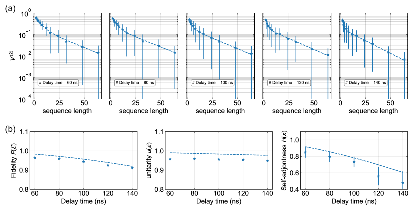
In the first experiment, we set the frequency of the local oscillator to and treat the qubit as a target qubit isolated from the qubit . The background noise of the isolated qubit is often phenomenologically modeled by the Lindblad Master equation given by
| (48) |
where represents the energy dissipation with the relaxation time , is an annihilation operator of the qubit, and represents the phase dissipation with the relaxation time . By solving the Eq. (48), we can obtain phenomenological predictions about the background noise corresponding to the delay time .
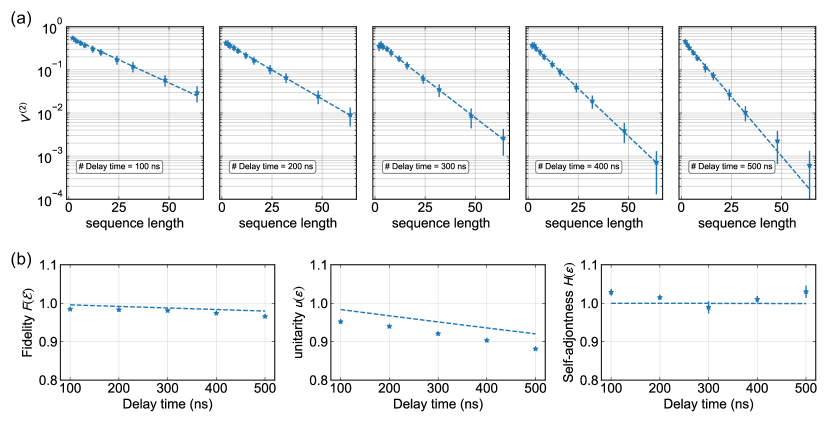
We sweep the delay time from to . The value obtained from the experiments is shown in Fig. 4 (a). We estimate the unitarity and the self-adjointness from through a fitting based on a sum of two exponentially-decaying curves given in Eq. (39). However, we observe single-exponential decays from the results. This indicates two possibilities. One is that the two decaying rates are nearly the same. The other is that one of the two decaying rates is much smaller than the other, so that one exponentially-decaying curve becomes quickly negligible as increases.
In our experiment, the former is the case because the average fidelity is high, which is confirmed from the -RB. We can analytically show that the two decaying rates typically coincide when the fidelity is sufficiently high. More specifically, we have (see Eq. (101) in Subsec.VIII.2)
| (49) |
to the first order of , where is the infidelity . This implies that the two decaying rates in Theorem 7 are approximately greater than and , respectively. Thus, if , which is indeed the case in our system, the two decaying rates are hard to distinguish, making the curve of a single-exponential decay.
We, hence, estimate the single-exponential decay rate from the experimental data of the -RB and derive and from
| (50) |
Here, is obtained from the estimated decaying rate, and from the -RB (See Eq. (39)).
The obtained fidelity, unitarity, and self-adjointness are summarized in Fig. 4 (b).
In calculating self-adjointness, we solved Eq. (28), where we substituted of the phenomenological prediction.
They reveal that the background noise of the isolated qubit has the unitarity that slowly decreases as the delay increases, while its self-adjoingness is nearly independent of the delay.
As we have explained in Subsec. IV.1, a problem may occur when the unitarity is high and the self-adjointness is low, which is not observed in this experiment. Hence, we conclude that the background noise in this case would not cause any problem toward the realization of QEC.
In the second experiment, we set the frequency of the local oscillator to and treated as a target qubit exposed to the noise induced by the adjacent qubit . In this experiment, no control pulses are applied to , so that is expected to remain in the state. This leads to a continuous rotation of the state vector of by the interaction Hamiltonian term of .
In this case, the background noise with the interaction Hamiltonian is modeled by the Lindblad Master equation written as follows,
| (51) |
providing a phenomenological model.
Similarly to the first experiment, we sweep the delay time from to . The delay time is set to a shorter time than the first experiment because the fidelity deteriorates due to the Z-rotation error. Since the Z-rotation error does not affect the unitarity, we conclude that the decay rate, which is less sensitive to the delay time than the other, corresponds to the unitarity. The results of the experiment are shown in Fig. 5 (a). As seen from the results, the curves obey double-exponential decay. From the two decaying rates, we obtain the unitarity and the self-adjointness as a function of the delay time as depicted in Fig. 5 (b). Note that, although the unitarity may seem different from the former experiment, it is merely due to the different time scale of the horizontal axis. The unitarities in the two experiments indeed coincide within the standard deviation (see, e.g, the delay time (ns)).
The experimental results qualitatively coincide with the phenomenological predictions obtained from Eq. (51) (see Fig. 5 (b)). However, the experimental values tend to be smaller. This indicates that there exist noise sources not included in the phenomenological model. The candidates of the additional noise sources are calibration errors in the gates, the initial thermal excitation rate of (), and the interaction of with adjacent qubits other than . Note that the initial thermal excitation of makes the noise time-dependent due to the relaxation, and hence, makes the result different from the theoretical prediction of the -RB.
Compared to the first experiment (Fig. 4), we observe from Fig. 5 that the fidelity and the self-adjointness quickly decrease as the delay time increases. The latter decreases especially quickly: at (ns). This implies that, even if the fidelity is moderately high ( at (ns)), the extra -rotation induced by the interaction with another qubit radically changes the property of the noise and makes the noise far from self-adjoint. Consequently, as the delay increases, the noise quickly becomes the one that cannot be approximated by any stochastic Pauli noise.
This result has an important implication toward a realization of QEC. As mentioned in Subsec. IV.1, theoretical studies of QEC commonly assume stochastic Pauli noises to numerically compute error thresholds and error rates. Our result implies that, when the interaction with another qubit is non-negligible, we cannot directly apply the theoretical predictions based on Pauli noises. This problem will be more prominent when the system size grows since, in a large system, a qubit interacts with more qubits in an uncontrolled manner, making the noise much less self-adjoint and much far from Pauli noises. To circumvent this, effective cancellation of the dipole interaction is of great importance in the further improvement since the dominant interaction between qubits should be originated from the electric dipole interaction.
This feature of the noise, i.e., interactions with other qubits induce small self-adjointness and the difficulty of approximating the noise by a Pauli noise, is expected to be common in any experimental systems. The -RB experiment and the self-adjointness offer a useful method and measure, respectively, to experimentally evaluate the noise in the system from this perspective.
VI Structure of the remaining paper
The remaining of this paper is organized as follows. In Sec. VII, a proof of Theorem 3 is provided. A brief introduction of representations of the unitary group is also provided before the proof. We then explain the higher-order RB in Sec. VIII, including the proof of Theorem 7. The methods used in the numerical analysis, and the experimental demonstrations are provided in Sec. IX. After we summarize the paper in Sec. X, we prove technical statements in Appendices.
VII Constructions of exact designs
In this section, we provide a proof of Theorem 3. We start with a brief introduction of representations of the unitary group in Subsec. VII.1, and prove Theorem 3 in Subsec. VII.2.
VII.1 Unitary -designs and representation theory
Unitary -designs are closely related to representations of the unitary group since the operator in the definition can be regarded as a representation of on with being the Hilbert space with dimension , i.e., . It is natural to consider irreps of the unitary group.
A well-known fact is that each irrep can be indexed by a non-increasing integer sequence , i.e. , of length . In particular, each irrep in can be indexed by an element of a set defined by
| (52) |
where and are the absolute value of sum of positive and negative ’s, respectively. Using this notation, the representation space is irreducibly decomposed into
| (53) |
where is the multiplicity of the irrep . Accordingly, the map is also decomposed into the irreducible ones .
Based on the irrep of the unitary group, a unitary -design can be characterized in a representation-theoretic manner: for any ,
| (54) |
The strong unitary -designs are similarly characterized in terms of irreps RS2009 . To this end, let be
| (55) |
where is not necessarily equal to . Then, a strong unitary -design satisfies
| (56) |
for any .
One of the merits in this characterization is that the right-hand-sides of Eqs. (54) and (56) are zero for all non-trivial irreps due to the Schur’s orthogonality relation, which states that, for any unitarily inequivalent irreps and ,
| (57) |
for any , where is the element of the matrix. By setting the irrep to a trivial irrep, i.e., for any , we have
| (58) |
for any non-trivial irrep . On the other hand, for any trivial irrep , it is trivial that
| (59) |
From these facts, (strong) unitary -designs can be defined in terms of representation as follows:
Definition 8 (Unitary designs in representation theory).
An ensemble of unitaries is an exact unitary -design if it holds for any irrep with that
| (60) |
An ensemble is a strong unitary -design if Eq. (60) holds for any irrep with .
VII.2 Proof of Theorem 3
We now prove Theorem 3, which states that defined by
| (61) |
is a strong unitary -design on . Here,
| (62) |
where and are strong unitary -designs on and , respectively, and is constructed by solving the zonal spherical function .
It suffices to show
| (63) |
for all non-trivial irreps indexed by . Note that the average over consists of the independent averages over all , further consisting of those over the strong unitary -designs and .
Let us first fix a non-trivial irrep and consider defined by
| (64) |
Since we consider only irreps , this average can be replaced with the averages over the product of the Haar measures on . That is,
| (65) |
To investigate , we consider the irreps of . Since is a subgroup of , each irreducible space of is decomposed into a direct sum of those of irreps of . For the same reason as in Definition 8, every non-trivial irrep of becomes zero by taking the average over . Hence, if the non-trivial irreducible representation space of does not contain trivial irreps of , . In contrast, if a non-trivial irrep of contains trivial irreps of , then the matrix elements of corresponding to the trivial irreps of are one, and the others are zero.
Trivial irreps of in a non-trivial irrep of were studied in a great detail since is an example of a Gelfand pair T1994 ; W2007 . It is known that the irreps of indexed by contains only one trivial irreps of , and that other irreps of contain no trivial irrep of GW2009 . Since trivial irreps are one-dimensional, we denote by a unit vector that spans the trivial irrep of in the spherical representation of . Then, we have
| (66) |
If , we immediately obtain from the definition of , which implies Eq. (63).
If , we define a matrix on () by
| (67) |
Importantly, for any , there exists at least one such that . This follows from the fact that
| (68) | ||||
| (69) |
where we have used the unitary invariance of and that the irrep is non-trivial, so that . Due to the intermediate value theorem, there always exists at least one unitary such that .
Using such and Eq. (66), it is straightforward to observe that . Furthermore, it follows that
| (70) | ||||
| (71) | ||||
| (72) |
We, hence, obtain
| (73) |
Thus, the finite set of unitaries satisfies the condition for the design, i.e., Eq. (63) for any non-trivial irrep , which leads to the statement that the set of unitaries defined by
| (74) |
is a strong -design on .
Finally, let us clarify the relation between and the zero of the zonal spherical function. To this end, we first observe that the matrix element of is the zonal spherical function . This can be checked by a simple calculation: for any and , we have
| (75) | ||||
| (76) | ||||
| (77) |
where the averages are all taken over . Thus, is bi--invariant, and so, is the zonal spherical function. This implies that is indeed a zero of the zonal spherical function.
Based on this fact, we can provide a matrix form of in the fixed basis in which a unitary in is represented as . To this end, it is important to notice that the bi-K-invariance of the zonal spherical function implies that it is characterized by the cosets of in . The cosets can be further identified with -dimensional subspaces corresponding to the support on which acts. For instance, the identity element in the coset of corresponds to the subspace spanned by the first vectors of the fixed basis. The matrix form of is obtained by specifying the relation between and the subspace corresponding to another representative of the coset.
To characterize the relation between two subspaces, we use the principal angles. For two subspaces and , let us refer to , where the minimum is taken over all unit vectors , as the minimum angle between and . The principal angles between two -dimensional subspaces and are then defined as follows: is the minimum angle between and , and is the minimum angle between and , where is a pair of the unit vectors that leads to .
The cosine of the principal angles between and the subspace corresponding to another representative in the coset determines the value of the zonal spherical function , and so, can be written as R2010 ; BNOZ2020 . See, e.g., Refs. JC1974 ; R2010 ; BNOZ2020 for the explicit form of as a polynomial of .
By solving the polynomial, we obtain the principal angles between and the subspace corresponding to the zero of . Recalling the definition of the principal angles and using the left- and right-invariance of the coset by any unitary in , we can take a matrix form of as follows:
| (78) |
where and , and is the identity matrix of size . Note that is not necessarily in this form since the coset is invariant under the action of .
VIII Higher-order RB
In this section, we investigate the higher-order RB in detail. We begin with a preliminary in Subsec. VIII.1 and explain several basic properties of the self-adjointness in Subsec. VIII.2. We consider the -RB for general and the -RB in Subsecs. VIII.3 and VIII.5, respectively.
VIII.1 Liouville representation
Let , , , and be normalized Pauli operators on one qubit, where normalization is in terms of the Hilbert-Schmidt inner product. For qubits, we introduce a vector () and use the notation that
| (79) |
We also denote by in this section.
The Liouville representation is a matrix representation of quantum channels, also known as the Pauli transfer matrix. See, e.g., Refs. WGHF2015 ; KLDF2016 ; DHW2019 . Let be a linear map from a set of all linear operators on a -dimensional Hilbert space to a -dimensional vector space that specifically maps to a canonical orthonormal basis vector . Since the map is linear, we have
| (80) |
for any linear operator . Note that .
Based on this vector representation of linear operators, a linear supermap can be represented by a matrix. The Liouville representation of a linear supermap is defined by
| (81) |
which is a regular matrix of size . The matrix element in the canonical basis of is given by
| (82) |
The vector and Liouville representations satisfy the following properties:
-
1.
,
-
2.
,
-
3.
(),
-
4.
,
-
5.
.
Properties of a linear supermap can be also expressed in terms of the Liouville representation. For instance, the linear map is TP if and only if and for any . Since we are interested in the CPTP map that represents a noise, its Liouville representation is always in the form of
| (83) |
where is a row vector of length with all elements being zero, is a column vector of length , called a non-unital part of the noise, and is a matrix. The non-unital part of the noise is the zero vector if and only if the map is unital, i.e., with being the identity operator.
In the Liouville representation, the fidelity parameter and the unitarity of a noisy CPTP map are given by
| (84) | ||||
| (85) | ||||
| (86) | ||||
| (87) |
respectively.
VIII.2 Properties of the self-adjointness
For a CPTP map , the self-adjointness and the self-adjointness parameter are defined by
| (88) | ||||
| (89) | ||||
| (90) |
where , and the last line is shown in Appendix D.
We first show the relation between and , i.e., Eq. (28) in Subsec. IV.1:
| (91) |
From the definition of , we have
| (92) |
By rewriting with , the first term in the right-hand side is expressed in terms of the unitarity , such as
| (93) |
By using the swap operator , and the property that for any matrices and , which is called a swap trick, it follows that
| (94) | ||||
| (95) | ||||
| (96) |
which leads to
| (97) |
Similarly, we obtain
| (98) |
from the facts that and that for any TP map .
From the definition of , it is straightforward to show that the self-adjointness parameter is given by
| (99) |
Combining these altogether, we arrive at
| (100) |
implying Eq. (91).
The self-adjointness parameter also satisfies the following properties. They are all shown in Appendix D.
-
1.
.
-
2.
if and only if . For a unital noise , if and only if the noise is self-adjoint ().
-
3.
if and only if for any , where are the Kraus operators of .
-
4.
the average gate fidelity is bounded from above by and :
(101)
VIII.3 A general expression for the -RB
We here show that the expectation value in the -RB has a general form of
| (102) |
where is a regular matrix depending on and , and is a regular matrix depending only on . As we will see below, labels the irreps of a -copy representation of the unitary group, and the size of the matrices is equal to the multiplicity of each irrep.
The expectation value is defined by
| (103) |
where is the average over all unitary sequences . Note that and that is the unitary channel defined by . In terms of the Liouville representation, we have
| (104) |
where we have used that , , and .
Noticing the -th power and the fact that each unitary is independently chosen from a unitary -design , we obtain
| (105) |
where is defined by
| (106) | ||||
| (107) | ||||
| (108) |
The last line follows since is an exact unitary -design.
To write down explicitly, let us consider the tensor- Liouville representation given by
| (109) |
where is the general linear group acting on the -dimensional vector space defined by
| (110) |
We denote the irreducible decomposition by
| (111) |
where labels the irreps, and is the multiplicity of the irrep labeled by .
The key observation is that
| (112) |
which simply follows from the unitary invariance of the Haar measure. This implies that , where is a set of all endomorphisms of that commute with the tensor- Liouville action of . It is well-known that is isomorphic to the direct sum of matrix algebras:
| (113) |
where is a set of all matrices over . Thus, the operator can be represented by a direct sum of matrices.
To obtain the explicit form of , let be a fixed decomposition of , and denote be the isomorphism from to . We also denote by the projection onto . Then, from the explicit form of the isomorphism, we have
| (114) |
where . Each element is given by
| (115) | ||||
| (116) | ||||
| (117) | ||||
| (118) | ||||
| (119) |
where we have used the irreducibility in the fourth line.
Consequently, it follows that
| (120) |
Substituting this into Eq. (105), we obtain
| (121) |
where the matrices are given by
| (122) |
This completes the proof.
VIII.4 The first-order RB
Let us briefly overview the -RB using an exact unitary -design, namely, the standard RB. We also explain how the result changes when the -design is an approximate one rather than the exact one.
In the -RB, the representation space is given by
| (123) |
We need to find a irreducible decomposition of under the action of a unitary group as . The Liouville representation is defined by . Hence, is irreducibly decomposed to
| (124) |
where
| (125) | |||
| (126) |
Denoting by and projectors onto and , respectively, we have
| (127) | ||||
| (128) |
where is the fidelity parameter. Note that is an exact unitary -design. We thus obtain that
| (129) |
where for .
When the -design is an approximate one , Eq. (128) holds only approximately. The degree of approximation depends on how we measure it, but we here assume that the design is -approximate when Eq. (128) holds up to -approximation. That is, we assume that
| (130) | ||||
| (131) |
where is some operator of . Note that standard definitions of approximate designs require harder criteria (see, e.g., Ref. L2010 ). In this case, instead of Eq. (129), we have
| (132) |
where
| (133) | |||
| (134) | |||
| (135) | |||
| (136) |
VIII.5 The second-order RB
We now focus on the -RB. Although the representation space in this case is
| (137) |
where we have used the notation that , it is not necessary to consider the whole space because we assume that the initial operator is traceless. This, together with the fact that the noise map is trace-preserving, implies that the operator remains traceless during the whole process. We also observe that the whole process is symmetric under the exchange of the first and the second spaces, each labeled by and in Eq. (137). Hence, in the analysis of the -RB, the relevant space is only the traceless symmetric subspace defined by
| (138) |
where . The irreducible decomposition of can be obtained by an extensive use of the result in Ref. HWW2018 (see Appendix C), based on which we explicitly compute .
It turns out that the situation differs depending on whether or . We, hence, deal with the two cases separately.
VIII.5.1 -RB in a single-qubit system
When , the irreducible decomposition of is given by
| (139) |
which is multiplicity-free. Here, and are
| (140) | |||
| (141) |
respectively, with . It is obvious that and .
This decomposition implies that the expectation is in the form of
| (142) |
where both and are given by
| (143) | |||
| (144) |
with being the projections onto . Since the projections can be explicitly constructed from Eqs. (140) and (141), we can compute .
First, we have
| (145) | ||||
| (146) | ||||
| (147) |
For , we start from the relation that
| (148) |
where is the projection onto the symmetric subspace of . The projection is also expressed by . Here, is the identity operator on and is the swap operator on defined by . Using the swap trick, we have
| (149) |
Moreover, from the direct calculations, we obtain
| (150) | |||
| (151) |
where . Further using the relations
| (152) | |||
| (153) |
we obtain from Eq. (148) that
| (154) | ||||
| (155) |
Altogether, we obtain
| (156) |
VIII.5.2 -RB in a multi-qubit system
For a multi-qubit system (), the traceless symmetric subspace is decomposed into four irreducible subspaces:
| (157) |
where and the others are given in Appendix C. Each irrep is multiplicity-free. We denote by the dimension of each subspace, which are
| (158) | |||
| (159) | |||
| (160) | |||
| (161) |
Since the decomposition is multiplicity-free, is a sum of four exponentially decaying functions. Furthermore, from the fact that , we obtain that . Hence, we have
| (162) |
where
| (163) | |||
| (164) |
with being the projections onto the irrep .
It is not clear whether each () has a clear physical meaning, such as being the unitarity. However, a linear combination of them does. To see this, we use the relation that
| (165) |
where . From this relation, we can show, by a calculation similar to the one-qubit case, that
| (166) |
Since , we obtain
| (167) |
We finally note that Tab. 1 in Subsec. IV.5 is obtained by constructing the orthonormal basis in each subspace , , and (see Appendix C). We also assume that the noise is weak, so that . Based on this assumption, we have
| (168) |
enabling us to compute for given initial and measurement operators.
IX Experimental realization of -RB
Based on the former sections, we explain in detail how we have experimentally implemented the -RB and estimated the self-adjointness of the noise in the system. In Subsec. IX.1, we provide the details of the numerical evaluation of the one- and two-qubit -RB discussed in Sec. V.1. The details of experiment is given in Subsec. IX.2.
IX.1 Numerical analysis
IX.1.1 Single-qubit systems
We explain the fitting procedure of the 2-RB on one-qubit systems in detail. The noise we consider is given by the following CPTP map:
| (169) |
which is characterized by three parameters , and . We particularly choose as for the fidelity parameter to be independent of the coherence parameter . Using the Liouville representation, it is straightforward to compute the fidelity parameter, the unitarity, and the self-adjointness parameter of this noise. They are, respectively, given by
| (170) | |||
| (171) | |||
| (172) |
As shown in Theorem 7, for one qubit is
| (173) |
To obtain Fig. 2 in Subsec. V.1, we first estimate the fidelity parameter from the -RB, i.e., by fitting and then obtain and from the fitting results of and the estimated value of . The fitting of is first performed based on Eq. (173) by regarding the coefficients and the two exponential decaying rates as free parameters. Then, we subtract the first exponential curve of Eq. (173) from the data and carry out the fitting of the second exponential curve again where we consider and the base of the second exponential curve as free parameters. This procedure is redundant, but turns out to improve the accuracy of the fitting because, in most cases, the first exponential decaying rate is larger than the second one, and thus the second exponential curve is clearly visible in the region of long sequence length.
We also estimate how many measurements and unitary sequences suffice to obtain a good estimate of the noise parameters. In Fig. 6, we provide for various numbers of measurement and samplings of unitary sequences. We observe that for both suffice to obtain a good estimate when , which corresponds to the gate fidelity .
When the number of measurements is small, experimental values are positively biased from theoretical values with the infinite number of samplings (see the figures in the top line of Fig. 6). This difference can be understood as follows. Let be the expectation value for a random sequence described by with the finite number of measurements. We describe the expectation value and variance of this random variable averaged over all choices of the unitary sequence as and , respectively. Note that this mean value is independent of , and this variance is inverse proportional to since is a linear combination of binomial distribution. is the expectation value of squared random variable , and its expectation value over random sequences is derived as
| (174) | ||||
| (175) |
Therefore, an experimentally obtained value with a finite number of measurements is positively biased by . In practice, we can remove the effect of this bias by increasing the number of sampling and using the region satisfying for fitting.
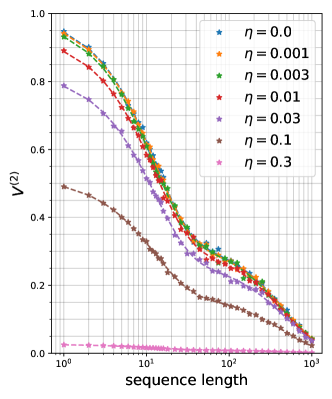
We finally check the robustness of the -RB on single-qubit systems against SPAM errors. Although the -RB is ideally SPAM-error free, the fitting may become harder with the existence of SPAM errors. Our analysis, however, reveals that this is unlikely the case. Here, we model the state-preparation error as and , and measurement error as readout bit-flip error, i.e., the POVM is where and is conditional probability. In this numerical experiments, we assume that and get 1000 samples and 1000 random sequences. We set the parameters .
The results are provided in Fig. 7 and Tab. 4. The relative errors of estimates for , and are within except for the estimate for when , thus the 2-RB is likely to work well even in realistic situations with SPAM errors as expected from the analytical studies.
| SPAM error | |||
|---|---|---|---|
| 0.0 | |||
| 0.001 | 0.986(5) | 0.9979(6) | 0.92(7) |
| 0.003 | 0.986(5) | 0.9978(5) | 0.92(1) |
| 0.01 | 0.987(0) | 0.9979(2) | 0.92(2) |
| 0.03 | 0.986(5) | 0.9980(1) | 0.92(8) |
| 0.1 | 0.986(5) | 0.9978(9) | 0.92(7) |
| 0.3 | 0.986(6) | 0.9981(8) | 0.92(7) |
| 0.9866 | 0.99793 | 0.9247 |
IX.1.2 Two-qubit systems
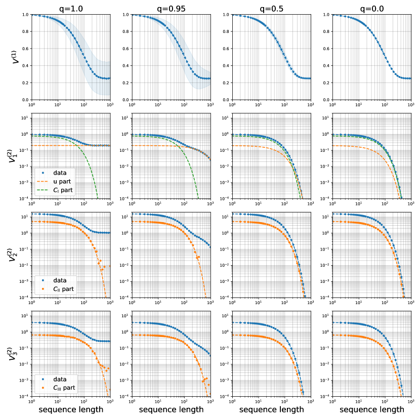
For two-qubit systems, we investigate the noise given by
| (176) |
where we set to . From Theorem 7, in this case shall be in the form of
| (177) |
and satisfy
| (178) |
With this setting, theoretical values are derived as follows.
| (179) | |||
| (180) | |||
| (181) | |||
| (182) | |||
| (183) |
from which the theoretical value of the self-adjointness parameter can be computed from Eq. (178).
A step-by-step fitting process of two-qubit systems is shown in Fig. 8 for . The numbers of measurement and samplings of unitary sequences are both set to . The fidelity parameters can be obtained from , which are plotted in the top line of the figure. In the figure, dashed lines are theoretical values, and the shaded area represents a standard deviation of each data. When is near to unity, standard deviations are large even when the sequence length increased. This is because the final quantum state is nearly pure state when , and probability distributions fluctuate randomly according to chosen random sequences. On the other hand, when , the final quantum state quickly converges to the maximally mixed state, and thus probability distribution becomes independent of the chosen random sequences.
We then fit four values step by step where initial and measurement operators and are chosen according to Tab. 1. The fitting results for several are shown in Tab. 5.
First, we obtain and from . The obtained results are shown in the second line of Fig. 8. The sampled data points and fitting results are shown as blue points and dashed lines, respectively. These lines are linear combinations of two exponentially decaying function. Exponential decays with coefficient and are shown as orange and green lines, respectively. While we can clearly see two exponential decays for coherent noise, i.e., in the case of , an exponential decay of part becomes dominant when noise becomes probabilistic. Even in this case, the fitting results are still reliable as shown in Tab. 5.
Then, we estimate from and from , where these initial and measurement operators are chosen from the third and fourth columns of Tab. 1. The obtained results are shown in the third and fourth lines of Fig. 8. In each figure, numerical data is plotted as blue circles and fitting results are shown as dashed lines. In each fitting process, only a single exponentially decaying term is unknown in advance. We showed unfitted exponential decay as orange circles and fitting results as dashed lines. Although accuracy of orange data becomes not reliable when its value becomes much smaller than the others, we can fit and reliably.
We calculate the averaged fidelity , unitarity , and self-adjointness from the fitting results. The processed values are shown in Tab. 6. We evaluate relative errors for all the plots with the same method as the single-qubit -RB, and confirm that the relative errors are below for all the cases of except the case when the theoretical value is exactly zero. While the relative errors of the self-adjointness become a few tens of percent in the case of , we can say that reliable values can be obtained when the fidelities of operations are sufficiently high. Note that, although standard deviations of the fitting results become large when is almost equal to , we confirmed that the fitted results are close to theoretical values even in such cases. Thus, we conclude that -RB works also for two-qubit systems.
IX.2 Details of the experiments
In this section, we provide the details of the experiments in Sec. V.2. A superconducting qubit can be regarded as a sort of the LC resonant circuit, where a Josephson junction is an effective inductance, and has the Hamiltonian equivalent to that of the one-dimensional free particle trapped in anharmonic potential.
| echo | ||||
|---|---|---|---|---|
| Q1 | ||||
| Q2 |
The parameter fields of the qubits are summarized in Tab. 7.
All unitary gates required in the -RB for a single-qubit case were implemented by two gates and three gates with an arbitrary rotation angle, which are implemented by the shaped microwave pulse (Half-DRAG) with the length lucero2010reduced and the Virtual- gates mckay2017efficient , respectively. The pre-measured averaged gate fidelity of the single-qubit Clifford gate is .
The single-shot qubit readout was performed via the impedance-matched Josephson parametric amplifier doi:10.1063/1.4886408 , and the assignment fidelity of the readout was .
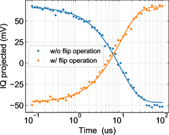
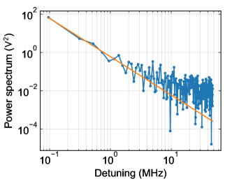
As supplemental experiments, T1 decay and Ramsey oscillation were observed to clarify the background noise source of Q1. The experimental results of the T1 decay is shown in Fig. 9, where the horizontal and the vertical axes represent the delay time and the projected value of the IQ readout signal, respectively. The blue and orange dots represent the experimental results with and without a flip operation just before measurement, respectively. The lines provide the fitting curves. As seen from the result, the T1 decay of Q1 follows exponential behavior, which is consistent with the expected behavior in isolated qubits.
The experimental results of the Ramsey oscillation is also given in Fig. 10, where the horizontal and vertical axes represent the detuning from the qubit eigenfrequency and the power spectrum of the Ramsey oscillation, respectively. The points connected by a blue line represent the experimental data, and the orange line provides a fitting curve. In the fitting, we did not take the data in the small power spectrum region () into account. This is because the noise floor derived from the white noise is dominant there. As seen from the result, the power spectrum of the Ramsey oscillation has no peaks other than the qubit eigenfrequency. From the fitting curve, it was found that the detuning from the qubit eigenfrequency () and the power spectrum of the Ramsey oscillation () are related as
| (184) |
This is consistent with the expected behavior when the transmon qubits are isolated well.
From the results of these supplemental experiments, we conclude that Q1 is not in the strong coupling regime with any noise source, which implies that the background noise of Q1 is time-independent. Thus, the requirements for -RB are met in our experimental system.
X Summary and Discussions
In this paper, we have provided an explicit constructions of exact unitary -designs for any . In particular, quantum circuits for exact unitary -designs on qubits have been provided for the first time. Our construction is inductive with respect to the number of qubits. Hence, all constructions obtained in this paper are inefficient when the number of qubits is large, implying that it is of practical use only when the size of the system is small.
As an application of exact unitary -designs on a small system, we have proposed the -RB, which enables us to experimentally estimate higher-order properties of the noise on a quantum system. Since the unitary designs are used in multiple times in a single run of the protocol, it is important for the design to be exact. After providing a general scheme of the -RB, we have studied the -RB in detail. It was shown that the -RB reveals the self-adjointness of the noise, a new characterization of the noise that we argue to play an important role in QEC especially when decoders are based on applications of Pauli operators. Our results have been demonstrated numerically, which shows that the -RB is experimentally tractable. We have then experimentally implemented the single-qubit -RB on the superconducting qubit system. From the experimental results, we found that the characteristics of the background noise of a qubit changes depending on the presence of the interaction with the adjacent qubits.
Our results open a number of future problems. Regarding the implementation of -designs, it is important to improve the efficiency. Despite that the inefficiency in our construction is likely to be intrinsic due to an inductive nature of the construction, the representation-theoretic method provides a way to searching more efficient ones. More specifically, the key in the construction is the relation between the representation of the whole unitary group and that of a certain subgroup of the unitary group. This indicates that finding the construction of exact unitary designs may be reduced to the problem of searching for a subgroup whose representation has a good relation to that of the whole unitary group.
It is also important to further develop the theory of the -RB protocol. In this paper, we have analyzed only the -RB in detail. It then turns out that self-adjointness of the noise can be revealed. It is of great interest to concretely investigate what characterization of the noise can be generally obtained from the -RB. In the context of QEC, it is also important to comprehensively analyze quantitative relations between the self-adjointness and the feasibility of QEC. Another promising future problem is to use exact higher-designs in the other RB-type protocols. The -RB is a straightforward generalization of the standard RB. However, there are numerous variant protocols HHFFW2019 , most of which, if not all, are based on the Clifford group that is an exact unitary -design. By extending such protocols to those with higher-designs, the noise on the system can be characterized in more detail.
XI Acknowledgements
The authors are grateful to H. Yamasaki and A. Darmawan for helpful discussions. Y. Nakata is supported by JST, PRESTO (No. JPMJPR1865). Y. Suzuki is supported by JST, PRESTO (No. JPMJPR1916). Y. Suzuki, K. Heya, Z. Yan, K. Zuo, S. Tamate., Y. Tabuchi, and Y. Nakamura are supported by JST ERATO (No. JPMJER1601) and by MEXT Q-LEAP (No. JPMXS0118068682).
References
- [1] A. Ambainis and J. Emerson. Quantum -designs: -wise independence in the quantum world. In Proc. IEEE Conf. Comput. 2007, page 129–140, 2007. arXiv:quant-ph/0701126v2.
- [2] I. Devetak. The private classical capacity and quantum capacity of a quantum channel. IEEE Trans. Inf. Theory, 51:44–55, 2005.
- [3] I. Devetak and A. Winter. Relating Quantum Privacy and Quantum Coherence: An Operational Approach. Phys. Rev. Lett., 93:080501, 2004.
- [4] B. Groisman, S. Popescu, and A. Winter. Quantum, classical, and total amount of correlations in a quantum state. Phys. Rev. A, 72:032317, 2005.
- [5] A. Abeyesinghe, I. Devetak, P. Hayden, and A. Winter. The mother of all protocols : Restructuring quantum information’s family tree. Proc. R. Soc. A, 465:2537–2563, 2009.
- [6] F. Dupuis, M. Berta, J. Wullschleger, and R. Renner. One-shot decoupling. Commun. Math. Phys., 328:251–284, 2014.
- [7] O. Szehr, F. Dupuis, M. Tomamichel, and R. Renner. Decoupling with unitary approximate two-designs. New J. Phys., 15:053022, 2013.
- [8] M. Horodecki, J. Oppenheim, and A. Winter. Partial quantum information. Nature, 436:673–676, 2005.
- [9] M. Horodecki, J. Oppenheim, and A. Winter. Quantum state merging and negative information. Comms. Math. Phys., 269:107–136, 2007.
- [10] A. Ambainis and A. Smith. Small pseudo-random families of matrices: Derandomizing approximate quantum encryption. In Proc. RANDOM’04, page 249, 2004.
- [11] P. Hayden, D. Leung, P. W. Shor, and A. Winter. Randomizing quantum states: Constructions and applications. Commun. Math. Phys., 250:371–391, 2004.
- [12] P. Sen. Random measurement bases, quantum state distinction and applications to the hidden subgroup problem. In 21st Annual IEEE Conference on Computational Complexity (CCC’06), pages 14–287, 2006.
- [13] F. G. S. L. Brandão and M. Horodecki. Exponential Quantum Speed-ups are Generic. Q. Inf. Comp., 13:0901, 2013.
- [14] R. Kueng, H. Rauhut, and U. Terstiege. Low rank matrix recovery from rank one measurements. Appl. Comput. Harmon. Anal., 42:88–116, 2017.
- [15] S. Kimmel and Y. Liu. Phase retrieval using unitary 2-designs. In 2017 International Conference on Sampling Theory and Applications (SampTA), pages 345–349, 2017.
- [16] R. Kueng, H. Zhu, and D. Gross. Distinguishing quantum states using Clifford orbits, 2016. arXiv:1609.08595.
- [17] M. Oszmaniec, R. Augusiak, C. Gogolin, J. Kołodyński, A. Acín, and M. Lewenstein. Random Bosonic States for Robust Quantum Metrology. Phys. Rev. X, 6:041044, 2016.
- [18] S. Boixo et al. Characterizing quantum supremacy in near-term devices. Nat. Phys., 14:595–600, 2018.
- [19] F Arute et al. Quantum supremacy using a programmable superconducting processor. Nature, 574:505–510, 2019.
- [20] A. Bouland, B. Fefferman, C. Nirkhe, and U. Vazirani. On the complexity and verification of quantum random circuit sampling. Nat. Phys., 15:159–163, 2019.
- [21] M. Oszmaniec, A. Sawicki, and M. Horodecki. Epsilon-nets, unitary designs and random quantum circuits. arXiv:2007.10885, 2020.
- [22] J. Emerson, R. Alicki, and K. Życzkowski. Scalable noise estimation with random unitary operators. J. Opt. B: Quantum semiclass. opt., 7:S347–S352, 2005.
- [23] E. Knill et al. Randomized benchmarking of quantum gates. Phys. Rev. A, 77:012307, 2008.
- [24] E. Magesan, J. M. Gambetta, and J. Emerson. Scalable and Robust Randomized Benchmarking of Quantum Processes. Phys. Rev. Lett., 106:180504, 2011.
- [25] E. Magesan, J. M. Gambetta, and J. Emerson. Characterizing quantum gates via randomized benchmarking. Phys. Rev. A, 85:042311, 2012.
- [26] J. Kelly et al. Optimal quantum control using randomized benchmarking. Phys. Rev. Lett., 112:240504, 2014.
- [27] S. Sheldon et al. Characterizing errors on qubit operations via iterative randomized benchmarking. Phys. Rev. A, 93:012301, 2016.
- [28] S. Garion et al. Experimental implementation of non-clifford interleaved randomized benchmarking with a controlled- gate. Phys. Rev. Research, 3:013204, 2021.
- [29] David C. McKay et al. Three-qubit randomized benchmarking. Phys. Rev. Lett., 122:200502, 2019.
- [30] A. D. Córcoles et al. Process verification of two-qubit quantum gates by randomized benchmarking. Phys. Rev. A, 87:030301(R), 2013.
- [31] Jay M. Gambetta et al. Characterization of addressability by simultaneous randomized benchmarking. Phys. Rev. Lett., 109:240504, 2012.
- [32] E. Magesan et al. Efficient measurement of quantum gate error by interleaved randomized benchmarking. Phys. Rev. Lett., 109:080505, 2012.
- [33] E. Onorati, A. H. Werner, and J. Eisert. Randomized benchmarking for individual quantum gates. Phys. Rev. Lett., 123:060501, 2019.
- [34] J. Helsen, I. Roth, E. Onorati, A. H. Werner, and J. Eisert. A general framework for randomized benchmarking, 2020. arXiv:2010.07974.
- [35] S. Popescu, A. J. Short, and A. Winter. Entanglement and the foundations of statistical mechanics. Nat. Phys., 2:754–758, 2006.
- [36] L. del Rio, J. Aberg, R. Renner, O. Dahlsten, and V. Vedral. The thermodynamic meaning of negative entropy. Nature, 474:61–63, 2011.
- [37] L. del Rio, A. Hutter, R. Renner, and S. Wehner. Relative thermalization. Phys. Rev. E, 94:022104, 2016.
- [38] P. Hayden and J. Preskill. Black holes as mirrors: quantum information in random subsystems. J. High Energy Phys., 2007:120, 2007.
- [39] Y. Sekino and L. Susskind. Fast scramblers. J. High Energy Phys., 2008:065, 2008.
- [40] L. Susskind. Addendum to Fast Scramblers. 2011. arXiv:1101.6048.
- [41] N. Lashkari, D. Stanford, M. Hastings, T. Osborne, and P. Hayden. Towards the fast scrambling conjecture. J. High Energy Phys., 2013:22, 2013.
- [42] P. Hosur, X.-L. Qi, D. A. Roberts, and B. Yoshida. Chaos in quantum channels. J. High Energy Phys., 2016:4, 2016.
- [43] D. A. Roberts and B. Yoshida. Chaos and complexity by design. J. High Energ. Phys., 2017:121, 2017.
- [44] Y. Nakata, E. Wakakuwa, and M. Koashi. Information leakage from quantum black holes with symmetry. 2020. arXiv:2007.00895.
- [45] K. A. Landsman et al. Verified quantum information scrambling. Nature, 567:61–65, 2019.
- [46] X. Mi et al. Information scrambling in computationally complex quantum circuits. 2021. arXiv:2101.08870.
- [47] P. Delsarte, J. M. Goethals, and J. J. Seidel. Bounds for systems of lines, and Jacobi polynomials. Philips Res. Rep., 30:91–105, 1975.
- [48] P. Delsarte, J. M. Goethals, and J. J. Seidel. Spherical codes and designs. Geom. Dedicata, 6:363–388, 1977.
- [49] A. Roy and A. J. Scott. Unitary designs and codes. Des. Code Cryptogr., 53:13–31, 2009.
- [50] A. Roy. Bounds for codes and designs in complex subspaces. J. Algebraic Combin., 31:1–32, 2010.
- [51] A. Roy and S. Suda. Complex spherical designs and codes. J. Comb. Des., 22:105–148, 2011.
- [52] E. Bannai, G. Navarro, N. Rizo, and P. H. Tiep. Unitary -groups. J. Math. Soc. Japan, 72:909–921, 2020.
- [53] D. P. DiVincenzo, D. W. Leung, and B. M. Terhal. Quantum data hiding. IEEE Trans. Inf. Theory, 48:580, 2002.
- [54] W. G. Brown, Y. S. Weinstein, and L. Viola. Quantum pseudorandomness from cluster-state quantum computation. Phys. Rev. A, 77:040303(R), 2008.
- [55] Y. S. Weinstein, W. G. Brown, and L. Viola. Parameters of pseudorandom quantum circuits. Phys. Rev. A, 78:052332, 2008.
- [56] D. Gross, K. Audenaert, and J. Eisert. Evenly distributed unitaries: On the structure of unitary designs. J. of Math. Phys., 48:052104, 2007.
- [57] G. Tóth and J. J. García-Ripoll. Efficient algorithm for multiqudit twirling for ensemble quantum computation. Phys. Rev. A, 75:042311, 2007.
- [58] C. Dankert, R. Cleve, J. Emerson, and E. Livine. Exact and approximate unitary 2-designs and their application to fidelity estimation. Phys. Rev. A, 80:012304, 2009.
- [59] A. W. Harrow and R. A. Low. Random quantum circuits are approximate 2-designs. Commun. Math. Phys., 291:257, 2009.
- [60] I. T. Diniz and D. Jonathan. Comment on “Random quantum circuits are approximate 2-designs”. Commun. Math. Phys., 304:281, 2011.
- [61] R. Cleve, D. Leung, L. Liu, and C. Wang. Near-linear constructions of exact unitary 2-designs. Quant. Info. & Comp., 16:0721–0756, 2016.
- [62] Y. Nakata, C. Hirche, C. Morgan, and A. Winter. Unitary 2-designs from random X- and Z-diagonal unitaries. J. Math. Phys., 58:052203, 2017.
- [63] A. W. Harrow and R. A. Low. Efficient Quantum Tensor Product Expanders and k-Designs. In Proc. RANDOM’09, Lecture Notes in Computer Science, pages 548–561. Springer Berlin Heidelberg, 2009.
- [64] F. G. S. L. Brandão, A. W. Harrow, and M. Horodecki. Local Random Quantum Circuits are Approximate Polynomial-Designs. Commun. Math. Phys., 346:397–434, 2016.
- [65] Y. Nakata, C. Hirche, M. Koashi, and A. Winter. Efficient Quantum Pseudorandomness with Nearly Time-Independent Hamiltonian Dynamics. Phys. Rev. X, 7:021006, 2017.
- [66] A. Harrow and S. Mehraban. Approximate unitary -designs by short random quantum circuits using nearest-neighbor and long-range gates. 2018. arXiv:1809.06957.
- [67] J. Haferkamp et al. Quantum homeopathy works: Efficient unitary designs with a system-size independent number of non-Clifford gates. 2020. arXiv:2002.09524.
- [68] E. Bannai, M. Nakahara, D. Zhao, and Y. Zhu. On the explicit constructions of certain unitary t-designs. J. Phys. A: Math. Theor., 52:495301, 2019.
- [69] R. Harper, I. Hincks, C. Ferrie, S. T. Flammia, and J. J. Wallman. Statistical analysis of randomized benchmarking. Phys. Rev. A, 99:052350, 2019.
- [70] P. D. Seymour and T. Zaslavsky. Averaging sets: A generalization of mean values and spherical designs. Adv. Math., 52:213 – 240, 1984.
- [71] P. Rabau and B. Bajnok. Bounds for the number of nodes in Chebyshev type quadrature formulas. J. Approx. Theory, 67:199 – 214, 1991.
- [72] G. Wagner and B. Volkmann. On averaging sets. Mon. Hefte. Math., 111:69–78, 1991.
- [73] E. Bannai and E. Bannai. A survey on spherical designs and algebraic combinatorics on spheres. European J. Combin., 30:1392 – 1425, 2009.
- [74] A. Bondarenko, D. Radchenko, and M. Viazovska. Optimal asymptotic bounds for spherical designs. Ann .of Math., 178:443 – 452, 2013.
- [75] Z. Cui, J. Xia, and Z. Xiang. Rational designs. Adv. Math., 352:541 – 571, 2019.
- [76] Z. Xiang. Explicit spherical designs. In preparation, 2020.
- [77] E. Bannai, Y. Nakata, T. Okuda, and D. Zhao. Explicit construction of exact unitary designs. 2020. arXiv:2009.11170.
- [78] R. A. Low. Pseudo-randomness and learning in quantum computation. PhD thesis, University of Bristol, 2010. arXiv:1006.5227.
- [79] D. Bump. Lie Groups. Springer-Verlag, New York, 2004.
- [80] R. Goodman and N. R. Wallach. Symmetry, representations, and invariants. Springer, Dordrecht, 2009.
- [81] A. T. James and A. G. Constantine. Generalized Jacobi Polynomials as Spherical Functions of the Grassmann Manifold. Proc. London Math. Soc., s3-29:174–192, 1974.
- [82] P. Chaugule et al. Schur polynomials do not have small formulas if the determinant doesn’t! 2019. arXiv:1911.12520.
- [83] F. Mezzadri. How to generate random matrices from the classical compact groups. Not. Am. Math. Soc., 54:592 – 604, 2007.
- [84] R. Kueng, D. M. Long, A. C. Doherty, and S. T. Flammia. Comparing experiments to the fault-tolerance threshold. Phys. Rev. Lett., 117:170502, 2016.
- [85] Y. R. Sanders, J. J. Wallman, and B. C. Sanders. Bounding quantum gate error rate based on reported average fidelity. New J. Phys., 18(1):012002, 2015.
- [86] Y. Suzuki, K. Fujii, and M. Koashi. Efficient simulation of quantum error correction under coherent error based on the nonunitary free-fermionic formalism. Phys. Rev. Lett., 119:190503, 2017.
- [87] S. Bravyi, M. Englbrecht, König R., and N. Peard. Correcting coherent errors with surface codes. npj Quantum Inf., 4:55, 2018.
- [88] A. S. Darmawan and D. Poulin. Tensor-network simulations of the surface code under realistic noise. Phys. Rev. Lett., 119:040502, 2017.
- [89] J. Wallman, C. Granade, R. Harper, and S. T. Flammia. Estimating the coherence of noise. New J. Phys., 17:113020, 2015.
- [90] C. D. Wilen et al. Correlated charge noise and relaxation errors in superconducting qubits. Nature, 594:369–373, 2021.
- [91] J. Han et al. Characterizing noise correlation and enhancing coherence via qubit motion. Fundam. Res., 1:10–15, 2021.
- [92] M. McEwen et al. Removing leakage-induced correlated errors in superconducting quantum error correction. Nat. Commun., 12:1761, 2021.
- [93] Matt McEwen et al. Resolving catastrophic error bursts from cosmic rays in large arrays of superconducting qubits. arXiv:2104.05219, 2021.
- [94] S. Tamate et al. Scalable packaging design for large-scale superconducting quantum circuit. Bull. Am. Phys. Soc., 2021.
- [95] J. Gambetta et al. Qubit-photon interactions in a cavity: Measurement-induced dephasing and number splitting. Phys.Rev. A, 74:042318, 2006.
- [96] R. A. Low. Large deviation bounds for -designs. Proc. R. Soc. A, 465:3289, 2009.
- [97] M. Takeuchi. Modern sphercal functions. American Mathematical Society, 1994.
- [98] J. A. Wolf. Harmonic Analysis on Commutative Spaces. American Mathematical Society, 2007.
- [99] B. Dirkse, J. Helsen, and S. Wehner. Efficient unitarity randomized benchmarking of few-qubit clifford gates. Phys. Rev. A, 99:012315, 2019.
- [100] J. Helsen, J. J. Wallman, and S. Wehner. Representations of the multi-qubit clifford group. J. Math. Phys., 59:072201, 2018.
- [101] E. Lucero et al. Reduced phase error through optimized control of a superconducting qubit. Phys. Rev. A, 82:042339, 2010.
- [102] D. C. McKay, C. J. Wood, S. Sheldon, J. M. Chow, and J. M. Gambetta. Efficient z gates for quantum computing. Phys. Rev. A, 96:022330, 2017.
- [103] J. Y. Mutus et al. Strong environmental coupling in a josephson parametric amplifier. Appl. Phys. Lett., 104:263513, 2014.
Appendix A Decomposing into two-qubit gates with arbitrary accuracy
We here explicitly show how to decompose defined by
| (185) |
into two-qubit gates with arbitrary precision under the assumption that ancillary qubits and an oracle that approximately compute from can be used.
More precisely, let be a -digit binary representation of with an accuracy , and suppose that an oracle works as for an arbitrary -qubit computational basis . From the oracle and an -qubit working register, we can construct an -qubit unitary gate which approximates as
| (186) |
where for all with two queries to the oracle and with two-qubit quantum gates whose number grows polynomially to .
This is done as follows. Suppose that an initial state is without loss of generality. Use the oracle to obtain . Apply two-qubit gates for to the quantum state where the first part of the tensor product in acts on the -th qubit of the second register and the latter part acts on the last register, then we obtain . We finally undo the second register with an oracle access to obtain .
Since , this process approximates within arbitrary accuracy by using sufficiently many number of ancillary qubits .
Appendix B A Clifford-based -design on two qubits
Denoting by () a single-qubit rotation around the -axis, we define a single-qubit rotation by
| (187) |
We also define a two-qubit rotation by
| (188) |
We also let be a fixed two-qubit unitary given by
| (189) |
where
| (190) | |||
| (191) | |||
| (192) | |||
| (193) | |||
| (194) |
Then, is an exact unitary -design on qubits, up to the numerical precision.
These numbers are obtained by numerically searching a zero of a function that is related to the -invariant functions. See Subsec. 9.3 of Ref. [77] for more details.
Appendix C Irreducible representations
We here provide the irreps of a unitary group on the vector space
| (195) |
under the action of with .
To this end, we index the irreps of unitary group by non-increasing integer sequences: , where , and (). The above representation contains the irreps indexed by , where , with being the sum of positive integers in , and .
For a given index , the dimension of the corresponding representation space is given by the Weyl’s dimension formula:
| (196) |
The multiplicity can be obtained from the Littlewood-Richardson rule. Since a single-qubit case () is special, we below consider the single-qubit case and the multi-qubit case separately.
The dimension and the multiplicity of irreps are summarized in Tab. 8 for one-qubit systems, and Tab. 9 for multi-qubit systems.
| Highest Weight | Dimension | Multiplicity | Irreducible spaces |
|---|---|---|---|
| Highest Weight | Dimension | Multiplicity | Irreducible spaces |
|---|---|---|---|
C.1 Single-qubit systems
To explicitly obtain all the irreps for one qubit, we start with the irreps of the Clifford group , which are provided in Ref. [100]. Since the Clifford group is a subgroup of the unitary group , irreps of the unitary group are obtained by taking the union of some irreps of the Clifford group. Since the dimensions of the irreps, both of the Clifford and the unitary groups, are known, we can check which irreps of the Clifford group should be combined by dimension counting.
First, from Theorem 1 in Ref. [100], the irreducible decomposition of in terms of is given by
| (197) |
Here, the important subspaces in our analysis are
| (198) | |||
| (199) | |||
| (200) |
See Ref. [100] for the definitions of the other subspaces, where the vector space is denoted by instead of . For instance, in our notation corresponds to in the notation of Ref. [100].
The dimension of each subspace is also given in Ref. [100] as
| (201) | |||
| (202) | |||
| (203) |
Comparing these with the dimensions of irreps of the unitary group, given in Tab. 8, it is clear that are also irreps of .
We can also show that is an irrep of . To this end, we show that , such that has a support on . Together with the dimension counting, it immediately leads to that is irreducible.
The statement is shown by construction. Let be a diagonal unitary matrix in . Using the simple relation that
| (204) | |||
| (205) |
it is straightforward to show that
| (206) |
Since and , we obtain the desired statement.
The fact that , , and are irreducible with respect to implies that so are the rest, i.e., , , and , due to the dimension condition. We hence obtain that the irreducible decomposition of :
| (207) |
where and are equivalent representations, and , , and are equivalent.
We finally mention the fact that the traceless symmetric ones are only and , which can be directly confirmed from their definitions. Thus, the traceless symmetric space is decomposed into irreducible subspaces as
| (208) |
which is multiplicity-free.
C.2 Multi-qubit systems
For , we also start with the irreps of the Clifford group . From Theorem 1 in Ref. [100], the irreducible decomposition by is given by
| (209) |
Similarly to the single-qubit case, by comparing the dimension of each subspace with those in Tab. 9, we obtain that and are the trivial irreps, and that , and are those corresponding to . We can also observe that and are also irrepds, corresponding to and , respectively.
We hence need to identify which of , , , , , and consist of the irrep with and the irrep with . This can be done again by dimension counting. From [100], the dimension of each subspace is given by
| (210) | |||
| (211) | |||
| (212) | |||
| (213) | |||
| (214) | |||
| (215) |
By a straightforward calculation, it can be shown that the only possible combination to satisfy the dimension condition that and is
| (216) | |||
| (217) |
We finally consider the irreducible decomposition of the traceless symmetric subspace . From the definitions of each subspace [100], we can easily check that the irreducible decomposition of by is given by
| (218) |
which is multiplicity-free. In the main text, we have denoted by for the simplicity of notation.
Appendix D Characterizations of a noise
We here show the following properties of the self-adjointness and the self-adjointness parameter .
-
1.
In the Liouville representation, the self-adjointness parameter is give by
(219) (220) -
2.
The self-adjointness parameter satisfies
(221) which immediately implies that .
-
3.
if and only if . For a unital noise, if and only if the noise is self-adjoint.
-
4.
if and only if for any , where are the Kraus operators of .
-
5.
The average gate fidelity is bounded from above by and :
(222)
We first show Eq. (219). Recalling that for any since is TP, we have
| (223) | |||
| (224) | |||
| (225) | |||
| (226) |
where is the swap operator on . Note that, in the last line, we have used the fact that is TP, also implying that is unital. We now use another expression of the swap operator, which is
| (227) |
which simply follows from the Schur’s lemma. Substituting this and using the relation that for any operators and , we obtain
| (228) |
On the other hand, it is straightforward to show that
| (229) | ||||
| (230) |
which follows from the definition of , i.e. . Hence, we have Eq. (219). Note that Eq. (220) follows simply from the definition of .
We next show Eq. (221), and the properties 3 and 4. The lower bound of in Eq. (221) is obtained from Eqs. (219) and (226), which lead to
| (231) |
Using the Kraus operators for and the swap trick, this can be rewritten as
| (232) |
which is not smaller than . The equality holds if and only if for any , which is the property 4. A simple instance of such a noise is a unitary noise that maps to .
The upper bound of in Eq. (221) is obtained from the relation that
| (233) |
which can be checked by a direct calculation. Since the left-hand side is non-negative, we have . About the property 3, it is obvious that if . The converse is shown as follows:
| (234) | |||
| (235) | |||
| (236) | |||
| (237) | |||
| (238) |
Note that the last line follows from the fact that is a real matrix in the Pauli basis.
We finally show the relation between the average fidelity , the self-adjointness parameter , and the unitarity , i.e. Eq. (222). To this end, we again use the fact that is a real matrix in the Pauli basis, leading to . We hence have
| (239) | ||||
| (240) | ||||
| (241) | ||||
| (242) | ||||
| (243) |
where the second inequality follows from the relation that for any matrix , and the last line from that is a real matrix, which implies that . Since and , we obtain Eq. (222).