Quantum complementarity from a measurement-based perspective
Abstract
One of the most remarkable features of quantum physics is that attributes of quantum objects, such as the wave-like and particle-like behaviors of single photons, can be complementary in the sense that they are equally real but cannot be observed simultaneously. Quantum measurements, serving as windows providing views into the abstract edifice of quantum theory, are basic tools for manifesting the intrinsic behaviors of quantum objects. However, quantitative formulation of complementarity that highlights its manifestations in sophisticated measurements remains elusive. Here we develop a general framework for demonstrating quantum complementarity in the form of information exclusion relations (IERs), which incorporates the wave-particle duality relations as particular examples. Moreover, we explore the applications of our theory in entanglement witnessing and elucidate that our IERs lead to an extended form of entropic uncertainty relations, providing intriguing insights into the connection between quantum complementarity and the preparation uncertainty.
I Introduction
Quantum mechanics imposes fundamental limits on an observer’s information gain in complementary measurements. In the light of Bohr’s complementarity principle [1], quantum systems possess mutually exclusive properties that are equally real, and a measurement to reveal one property would inevitably preclude all the complementary ones. Characterizing this subtle relationship between measurement strategy and information gain is significant for the sophisticated manipulation of quantum measurements in various tasks, from demonstrating genuine nonclassical features of quantum objects to general quantum information processing.
Wootters and Zurek [2] proposed the first quantitative statement of complementarity relation by taking an information-theoretical perspective into the competitive tradeoff between the wave-like and particle-like behaviors of single photons. This kind of wave-particle duality relations (WPDRs) are currently expressed in a concise inequality form [3, 4, 5, 6] for photons within the Mach-Zehnder interferometer (MZI; see Fig. 3). For example, Jaeger et al [4] and Englert [6] obtained the duality relation between fringe visibility (wave property) and path distinguishability (particle property) . It is thus obvious that better which-way information implies less wave information, and vice versa.
Heisenberg’s uncertainty principle [7] is another fundamental concept in quantum mechanics which captures similar underlying physics of complementarity. It states that outcomes of specific measurements, e.g., position and momentum of a single particle, cannot be predicted with certainty simultaneously. Modern formulations of the uncertainty principle typically use entropic uncertainty measures [8, 9] due to their operational significance and the widespread applications [10] of entropic uncertainty relations (EURs), e.g., in the security analysis of quantum protocols [11, 12, 13].
The connections and contrasts between uncertainty and complementarity have been intensively debated [14, 15, 16, 17, 18, 19, 20]. It has been wondered whether novel complementarity relations can be derived directly from the well-studied and already-proven EURs. Particularly, Coles et al [20] proved that several WPDRs in the two-way interferometer can be equivalently reformulated as EURs for complementary observables. Thus two fundamental concepts of quantum mechanics are unified in this simple case.
Nevertheless, entropy is a natural measure of lack of information regarding only observation-independent properties and becomes conceptually inadequate [21] for quantum properties which are contextual and do not exist prior to measurements [22, 23]. To avoid this dilemma, Brukner and Zeilinger proposed an operationally invariant information measure of quantum systems [24]. It is naturally aligned with the concept of complementarity as being elegantly defined as the sum of individual measures of information gain over a complete set of mutually unbiased bases (CMUBs) [25, 26, 27, 28]—complementary bases—independent of particular choices of CMUBs and invariant under unitary time evolution. These intriguing properties inspired a series of insightful investigations [29, 30, 31, 32, 33, 34, 35, 36], including quantum state estimation [29, 30] and uncertainty relations for MUBs [34, 35].
In this paper, we adopt the operationally invariant information measure [24] and develop a general framework for characterizing quantum complementarity beyond WPDRs, in terms of basic limits on one’s ability to gain information about quantum systems through complementary measurement setups, i.e., information exclusion relations (IERs). We emphasize that when considering generalized measurements, identifying certainty of outcome statistics with information gain or visibility of physical property faces conceptual challenge—an outcome predictable with 100% certainty not necessarily reflects the complete information of the measured system. In contrast to IERs [37, 38, 39, 40, 41] that utilize entropic mutual information or deriving complementarity relations from EURs [20], our theory applies to generalized measurements and well captures the complete information of quantum systems as conserved quantities comprised of complementary pieces, highlighting the interplay between different pieces of information and their complementary nature.
This paper is structured as follows. In Sec. II, we introduce some preliminary notations. In Sec. III, we propose a measure of information gain in individual measurements while formalizing the concept of complementary information. In Sec. IV, we proceed to establish IERs which restrict one’s weighted sum of information gains over multiple measurements, with and without quantum memory respectively. In Sec. V, we show how our IERs lead to tight WPDRs. In Sec. VI, we discuss practical applications of our IERs. Finally, we briefly conclude this work in Sec. VII.
II Preliminary
On a -dimensional Hilbert space , each generalized measurement, i.e., positive-operator-valued measure (POVM), is a collection of positive semi-definite operators (called effects) that sum up to the identity operator: and . In particular, the measurement of a nondegenerate observable is described by rank-1 projectors onto its eigenvectors, i.e., rank-1 projective measurement. When a quantum state is measured, the outcome probabilities are given by Born’s rule, .
The Choi-Jamiołkowski isomorphism [42] allows us to represent each operator on as a vector of the product space :
| (1) | ||||
where is the maximally entangled isotropic state and denotes the partial trace over the second space. A useful property of Eq. (1) that will be exploited is that holds for any two operators and on .
III Measure of information gain
In the light of Kochen-Specker’s theorem [22] (see also Ref. [23]), it is impossible to assign a definite noncontextual value to every quantum observable. During a measurement, all that an observer has is the probabilistic occurrence of one outcome (labeled contextual value 1), which simultaneously negates the occurrence of other outcomes (labeled contextual values 0). The information content of quantum systems is thus reflected in the statistics of these contextual binary strings.
Consider an experimental setup to perform the measurement on individual copies of a quantum state that is unknown to the experimenter. Each time the th outcome occurs, the experimenter gets a squared deviation from the expectation for the completely mixed state—least information state—or gets otherwise. After repeating the experiments large enough times, the total squared deviation is , which consists of two contributions . Wherein is the total uncertainty (variance), which determines the width of the confidence interval for estimating the outcome probabilities .
What truly discriminates the measured state from the completely mixed state, on the other hand, is the total squared bias . We suggest the measure of information gain on the state in each individual trial of the measurement to be the sum of mean squared bias over all outcomes
| (2) |
In the above, we leverage the isomorphism (1) to define the view operator of a measurement as
| (3) |
where is traceless, or equivalently, is orthogonal to . View operators are positive semi-definite, on the -dimensional subspace of orthogonal to , and vanish for trivial POVMs whose effects are all proportional to the identity, .
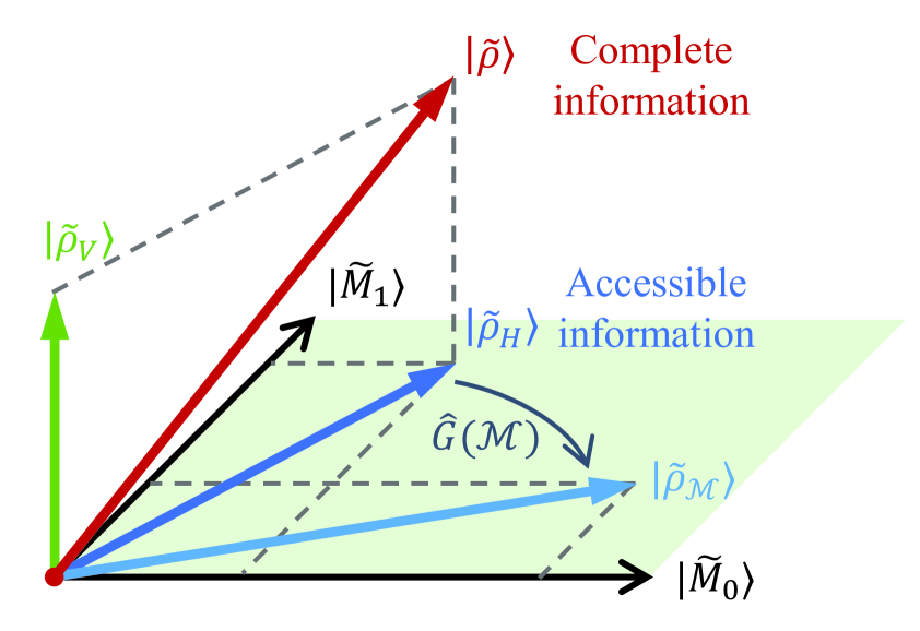
Now we are able to formalize our idea of complementary information. Let , observe that the outcome probabilities of a measurement on the state are encoded in the expansion coefficients of the vector under the basis . The vector encodes the complete information of if lies in the subspace of on which the view operator is invertible, whereas if is orthogonal to that space, vanishes and cannot be employed to distinguish from the completely mixed state (see Fig. 1 for an illustration of the geometric relations between the above vectors). In the sense above, two nontrivial measurements and satisfying
| (4) |
are complementary since, if the complete information of is accessible through , then no information gain is accessible through , and vice versa. We prove in Appendix. A that measurements in mutually unbiased bases (MUBs) [25, 26, 27, 28] are complementary.
It is worth mentioning that the combined view operator associated with a set of POVMs on can be positive definite (invertible) on . In this case, no POVM can be complementary to all POVMs of simultaneously. This means that is informationally-complete and offers a complete view to all -dimensional quantum states. Utilizing the isomorphism (1), arbitrary unknown state can then be reconstructed from the vector encoding the outcome statistics as follows
| (5) |
For further readings on the topic of state estimation, we recommend Refs. [43, 44].
Interestingly, the combined view operator associated with CMUBs of , i.e., mutually unbiased bases (MUBs) [25, 26, 27, 28], is simply the identity operator on (see Appendix. A). Thus the operationally invariant measure [24] of complete information content contained in quantum states can be restateted in our language as
| (6) |
This measure naturally coincides with Bohr’s idea [1] that only the totality of complementary properties together exhausts the complete information of objects.
IV Information exclusion relations
To formulate quantum complementarity into information exclusion relations, next we focus on the measurement scenarios where distinct measurements on individual copies of a quantum system are selected with biased (non-uniform) probabilities.
IV.1 Local information exclusion relations
Theorem 1. For a set of measurements with selection probabilities , the average information gain on the state satisfies
| (7) |
where is the average view operator and denotes the operator norm, i.e., the largest eigenvalue of an operator.
Theorem 1 limits an observer’s weighted average information gain over multiple measurements to be less than a proportion of the complete information content (6) contained in quantum states. We show in Appendix. A that for a number of rank-1 projective measurements. To be more precise, for nondegenerate observables with one or more common eigenstates we have and the rightmost side of Eq. (7) is achieved by density operators whose eigenvectors corresponding to positive eigenvalues form a subset of the common eigenstates of observables, which means that no state-independent information exclusion exists. On the other hand, we have for MUBs. Particularly, for random measurements in one of MUBs, , thereby . We therefore see that the average information gain is rather limited with an increasing number of MUBs.
Example. For random measurements on a qubit in one of two bases and , Eq. (7) gives . Here, is the maximal overlap between bases and in this simple example . By definition, holds for MUBs, while for compatible bases .
We remark that for those measurement strategies with which the associated view operator , the rightmost side of Eq. (7) can be achieved by any density operator on . Typical examples include random measurements in CMUBs, random selection of measurements from a complete set of mutually unbiased measurements [45] and other design-structured POVMs [46, 47, 48, 49, 50, 51] (see Appendix. A for details).
IV.2 Information exclusion relations with memory
We move on to investigate the basic limits on an observer’s information with respect to measurements on a distant quantum system, given access to another system (called memory). To illustrate, let us consider the guessing game [12] involving two participants, Alice and Bob. As depicted in Fig. 2a, in the beginning, Bob prepares a bipartite system in the state , and sends subsystem A to Alice. Upon receiving subsystem A, Alice chooses a measurement according to the value of a random variable drawn from the probability distribution , and announces her choice to Bob. Bob’s win condition is to guess the final state on Alice’s side correctly.
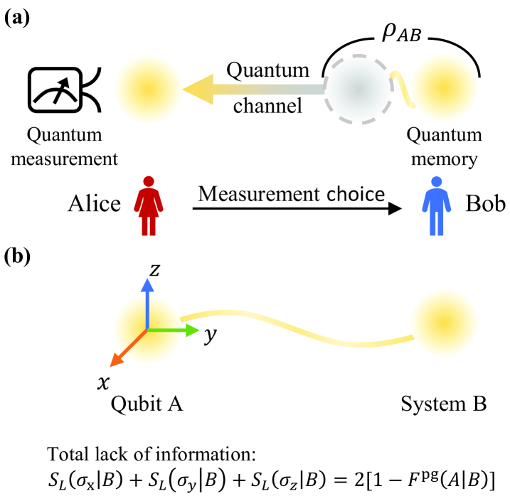
To quantify Bob’s lack of information about system A while possessing a memory system B, we define the conditional linear entropy as below
| (8) |
Here, is the recoverable entanglement fidelity with which can be transformed into a maximally entangled state through the pretty good recovery operation on system B [52, 53], and denotes the dimension of system A. In the case of a product state , system B offers no side information about system A and Eq. (8) reduces to the linearized entropy , i.e., the complement of the information content (6) contained in the state . More generally, according to the data-processing inequality [54, 55] we have , thereby a memory helps to reduce Bob’s ignorance. Further, is necessarily entangled if , since one’s ignorance about the overall system in a separable state does not increase with the removal of any its local subsystem [56, 57].
For brevity, we will focus on rank-1 projective measurements. Bob has no direct access to system A once it is sent to Alice, his understanding of the overall system when Alice chooses the th measurement is described by the classical-quantum state
| (9) |
where denotes the th effect of the th POVM and are the measurement outcomes stored in a classical register. Then, the conditional linearized entropy (8) evaluated on the classical-quantum state (9), denoted , measures Bob’s ignorance about Alice’s measurement outcomes. Indeed, is now precisely the probability for Bob to correctly guess Alice’s measurement outcome by performing the pretty good measurement on system B [58, 59].
Theorem 2. Suppose describes a bipartite system and are rank-1 projective measurements on system A with selection probabilities . The average conditional linearized entropy is bounded below by
| (10) |
We prove in Appendix. B a result that is valid for more general measurements. Like the memoryless IER (7), Eq. (10) becomes an equality saturated by arbitrary bipartite state if the equality holds. Consequently, in the absence of information exchange with environments or between systems A and B, Bob’s total information with respect to measurements on system A in CMUBs, as well as other design-structured measurements [46, 47, 48, 49, 50, 51], is time-invariant.
Impressively, the r.h.s. of Eq. (10) is a product of two independent terms controlled by Alice and Bob respectively. The first term, , is a state-independent signature of information exclusion and Alice is free to manipulate it through her measurement strategy. It varies in the range when the number of observables under consideration is . To keep her measurement outcomes secret, Alice should avoid measuring observables that share a common eigenstate (), as Bob can completely eliminate his uncertainty by preparing system A precisely in that eigenstate. In contrast, Bob’s uncertainty will be maximized if Alice randomly selects one of MUBs (). The special case when Alice chooses to measure the Pauli observables of a qubit is illustrated in Fig. 2b. We need to mention here that a set of MUBs may not exist for sufficiently large , and numerical methods can be utilized to maximize the exclusivity in such cases.
On the other hand, the second term decreases monotonically with the recoverable entanglement fidelity of the initial state . Bob’s pretty good guessing probability [58, 59] would be less than 1 whenever . However, he can prepare an appropriate entangled state such that this fidelity enables him to guess the outcomes of measurements on system A with high probability. Indeed, it is well known that maximally entangled states provide perfect side information. For example, two systems in the state are perfectly correlated with no local information content at all, , whereas the joint information content is maximal. This leads to , namely, the correlation between A and B is strong enough to completely remove Bob’s uncertainty. Just as is mentioned in Refs. [24, 21], the information content of a maximally entangled state is “exhausted in defining the joint properties” and “none is left for individual systems”.
V Origin of tight WPDR
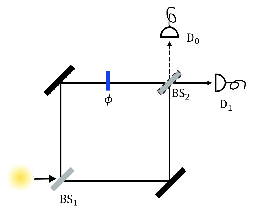
We argue that the tight WPDRs are particular examples of the IERs (7) and (10) for complementary observables. To see this, let us consider two complementary setups of the Mach-Zehnder interferometer depicted in Fig. 3: (i) the second beam splitter is removed to gain the path information of single photons inside the interferometer (let denote the associated path observable with binary outcomes “” and “”, corresponding to clicks in detectors and respectively ); (ii) BS2 is inserted in and the phase shift is adjustable to reveal wave properties of photons (let denote the associated wave observable with binary outcomes “”). It takes some calculation (see Appendix. C) to see that Eq. (7) leads to the equality
| (11) |
where denotes the average of observable , and and are the respective information gains (2) for measuring the path and wave observables in the qubit .
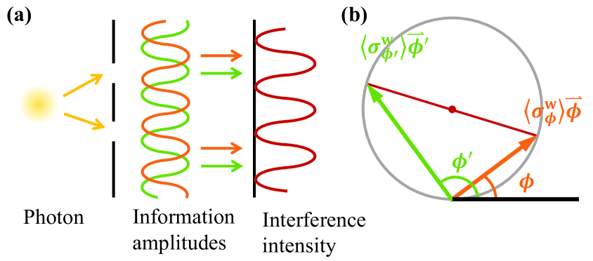
Observe that the information gain regarding an individual wave observable oscillates as the phase shift varies, Eq. (11) essentially depicts an interference pattern of the wave information. To make it clearer, let and be two real unit vectors at an angle of . Eq. (11) can then be restated as
| (12) |
It is interesting to note that the average values of wave observables behave like the “amplitudes of wave information” and interfere with each other, see Fig. 4a. Notably, the average interference intensity on the r.h.s. of Eq. (12) disappears if the photon exhibits particle property only—the complete information content of is accessible through measuring the path observable or, formally, . In this view, (see the case in the preceding equation) emerges as a measure of wave property which can be determined by measuring two complementary wave observables.
Conventionally, the wave property is frequently quantified by the fringe visibility [3, 4, 5, 6]
| (13) |
where is the probability that the th detector clicks when the observable is measured. We remark here that the average interference intensity is precisely half of the fringe visibility squared, i.e., (see also Fig. 4b for an illustration). Combined with the squared path distinguishability , we then arrive at the WPDR [60]. We therefore see that the WPDR originates from the IER for three complementary observables, including the path observable and two wave observables with phase difference satisfying .
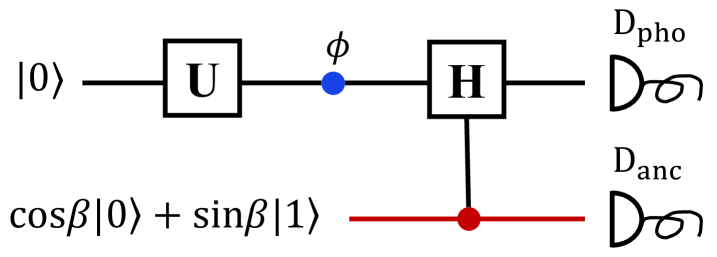
Theorem 1 applies also to the quantum delayed-choice experiment [61], where complementary properties of photons are measured in a single experimental setup. As shown in Fig. 5, the presence of BS2 is controlled by an ancilla qubit, the value of which determines whether to reveal the wave property or particle property. In this case, Eq. (7) limits an observer’s weighted average information gain about three complementary observables, with (unnormalized) weights for the path observable and for the wave observables. Therefore, the true nature of complementarity does not prohibit the observation of complementary properties in a single measurement setup, but necessarily restricts one’s simultaneous information gain about them.
Another interesting issue concerns the WPDRs when an observer has side information about single photons in the Mach-Zehnder interferometer, but without direct access to them. Let us consider two photons in the bipartite state . As a measure of information about photon A conditioned on photon B, we turn to the complement of the conditional linearized entropy (8) below
| (14) |
This is non-negative and reduces to the complete information of the reduced state , when is a product state.
We derive in Appendix. C the following generalization of Eq. (12),
| (15) |
Here, is the “amplitude of conditional information” which connects to the conditional information through its squared modulus .
Equation (15) manifests the interference pattern of conditional information amplitude, with the r.h.s. of it being the interference intensity. Combining the average intensity (wave property) with the conditional which-way information (particle property) , we then obtain the WPDR . Again, we see that a tight WPDR saturated by all bipartite systems with dimension arises from an IER for three complementary observables, wherein two complementary wave observables constitute the complete description of wave property.
VI Discussions
Our theory for characterizing information complementarity from a measurement-based perspective enables us to analyze the behaviors of quantum systems through their manifestations in versatile measurement setups, without delving into the exhaustive calculations with quantum state parameters. As two examples, we explore the implications of our IERs (7, 10) for entanglement detection and EURs respectively.
VI.1 Entanglement detection
Quantum correlation tends to suppress the local information content contained in individual subsystems. For example, a pair of maximally entangled qubits possess only joint properties in the sense that each single qubit is in the completely mixed state. We introduce the correlation measure for local measurements on individual copies of the bipartite state , where denotes the th effect of the th measurement and are the correlation detection operators. We show in Appendix. D the following.
Theorem 3. For any bipartite separate state , it holds that
| (16) |
where is the state-independent upper bound on local information gain given by Eq. (7).
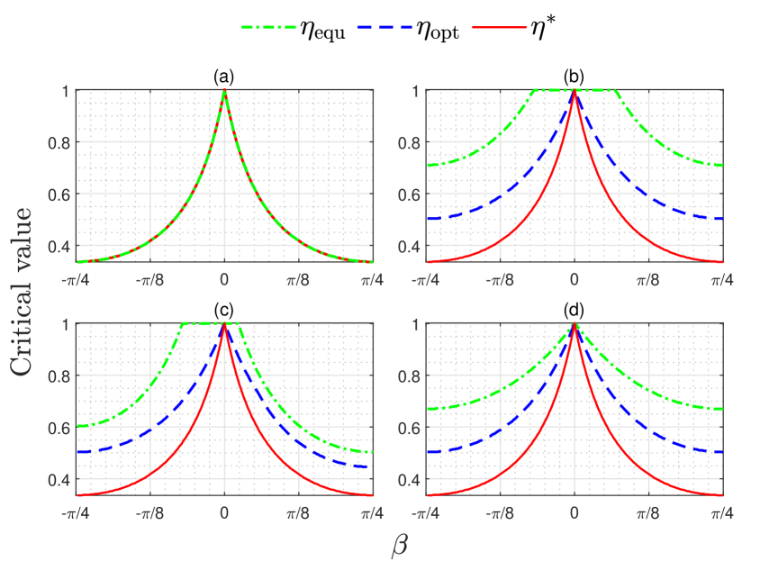
Consequently, a violation of Eq. (16) necessarily indicates the presence of entanglement. As a concrete example, we can apply Eq. (16) to the mixture of a pure two-qubit state and white noise:
| (17) |
Note that the noiseless state is entangled as long as . Now the question is how much noise it can resist from being separable, i.e., the critical value of below which ceases to be entangled. In Fig. 6, we present numerical results regarding the critical values and for the state (17) to violate Eq. (16), under measurements with equal weights and optimized weights respectively. As depicted, three complementary observables with equal weights are enough to detect all the entanglement . For more general observables , an optimization over the weights yields better performance.
VI.2 Implications for EURs
Entropic uncertainty relations (EURs) that take into account information leakage from a memory system play a crucial role in various aspects of quantum information processing [10], particularly in the security analysis of quantum protocols [12]. However, existing EURs [10] are thus far limited since they are restricted to providing lower bounds on simply entropy sums. On a conceptual level, there is no reason to assign equal weights, instead of biased weights, to different measurements. Based on Theorem 2, we have the following lower bounds on the weighted sum of entropies over multiple measurements (see the proof in Appendix, E).
Theorem 4. Suppose describes a bipartite system and are rank-1 projective measurements to be performed on system A with selection probabilities . The smooth minimum entropy evaluated on the state (9) satisfies , where
| (18) |
The conditional smooth minimum entropy [62] (see also Ref. [10]) is a fundamental tool for the security analysis of quantum protocols. In quantum cryptographic protocols where an eavesdropper aims to know an experimenter’s measurement outcomes by probing a memory system, the weighted EURs we introduced provide guidance for adjusting the probabilities of selecting distinct measurements to minimize potential information leakage. It is conceivable that equal selection probabilities are not optimal for biased measurements. Optimized selection probabilities are thus crucial for elaborating the measurement strategies to enhance security and achieve stronger levels of protection. Importantly, this optimization does not require additional quantum costs and can be easily done on a classical computer.
VII Conclusion
In summary, we have developed a general approach to formulate the complementarity principle quantitatively in terms of basic limits on one’s ability to gain information on quantum systems under versatile measurement setups, with and without memory respectively. Our framework sheds new light on the interpretation of wave-particle duality for single photons in the two-way interferometry experiments from an information-theoretical perspective. Extending this interpretation to multi-path interferometers presents an intriguing avenue for future investigation. Moreover, our IERs have direct applications in certifying genuine quantum features of physical systems, such as entanglement detection based on local measurement outcomes. An extended form of EURs can also be derived from our IERs, which could offer practical advantages in various quantum information processing.
Acknowledgements.
This work is supported by the National Natural Science Foundation of China (Grants No. 12175104 and No. 12274223), the Innovation Program for Quantum Science and Technology (2021ZD0301701), the Natural Science Foundation of Jiangsu Province (No. BK20211145), the Fundamental Research Funds for the Central Universities (No. 020414380182), the Key Research and Development Program of Nanjing Jiangbei New Area (No. ZDYD20210101), the Program for Innovative Talents and Entrepreneurs in Jiangsu (No. JSSCRC2021484), and the Program of Song Shan Laboratory (Included in the management of Major Science and Technology Program of Henan Province) (No. 221100210800-02).Appendix A View operator and properties
Consider a set of POVMs assigned with weights . We define the associated average view operator to be
| (19) |
where is traceless, or equivalently, is orthogonal to . View operators are positive semi-definite, on the -dimensional subspace of orthogonal to , and vanish for trivial POVMs whose effects satisfy .
The matrix representation of under an orthonormal basis of takes the form
| (20) |
Here, the matrix elements of are given by , with being a bijection from the labels of POVM effects to the labels of the basis vectors . Note that the positive eigenvalues of are identical to those of the Gram matrix for the vectors , that is, . To obtain eigenvalues of a view operator , it will be enough to deal with the Gram matrix , whose elements are .
Claim 1. POVMs that form a design structure are mutually complementary.
Claim 2. The combined view operator associated with a complete set of design-structured POVMs is proportional to the identity operator on .
Claim 3. The average view operator of a set of MUBs with weights satisfies .
Proof. Design-structured measurements include complete sets of mutually unbiased measurements (MUMs) [45], general symmetric-informationally-complete POVMs [49, 50, 51], POVMs from equiangular tight frames [48] and POVMs from general quantum designs [46, 47]. Without loss of generality, we prove the above claims for MUMs. MUMs [45] are -outcome POVMs satisfying , , and for all and . Here is called the efficiency parameter, wherein corresponds to projective measurements in MUBs [25, 26, 27, 28].
Consider the view operator associated with a set of MUMs [45] on , according to Eq. (20) the corresponding Gram matrix is given as
| (21) |
According to Eq. (21), obviously two MUMs are complementary since whenever . Next, let us focus on the submatrix
| (22) |
where denotes the matrix satisfying for all . This submatrix (22) has identical nonzero eigenvalues , thus the view operator of a complete set of MUMs (CMUMs) has identical nonzero eigenvalues. In other words, , with being the identity operator on the -dimensional space . Claim 3 follows from the fact that MUBs (i.e., MUMs with efficient parameter ) are complementary, thus .
Claim 4. For arbitrary -outcome POVMs on that consists of equal-trace effects (ETE-POVMs), i.e., , we have .
Claim 5. For any set of -outcome ETE-POVMs on , .
Claim 6. For a number of -outcome ETE-POVMs on with equal weights, iff the overlap matrix , defined as , is reducible.
Proof. Consider the Gram matrix . We can rewrite it as , where is referred to as the overlap matrix, and for all . Note is doubly stochastic, i.e., , its first eigenvalue (arranged in descending order) must be . Moreover, the corresponding eigenvector is also an eigenvector of which corresponds to the unique nonzero eigenvalue of . Immediately , and . Claim 5 follows directly from Claim 4. Further, considering that the matrix is doubly stochastic, according to Theorem 3.1 of Ref. [63] we have iff is reducible.
Appendix B Proof of Theorem 2
Let be a set of generalized measurements such that the POVM effects of each measurement are equal-trace, i.e., , where denotes the number of effects in the th POVM. After Alice performed the th measurement on system A, Bob’s understanding of the overall system is then described by the classical-quantum state
| (23) |
Here, are the Kraus operators [64] which satisfy by definition.
To prove Theorem 2, we only need to show the operator
| (24) |
is positive semi-definite on the space , where is an orthonormal basis of and . Notice that the measurement-induced local transformation commutes with the map , from we have
| (25) |
where . This leads us to
| (26) |
In the case of rank-1 projective measurements, are equal to the dimension of system A. With Eq. (26) Theorem 2 is already obvious.
Next, we proceed to show . Observe the operator below is positive semi-definite
| (27) | ||||
and, accordingly, so does its partial transpose over the second space
| (28) |
In the above
| (29) |
and
| (30) | ||||
Let be the operator when defined on the space . Similarly, and denote the same density operator but defined on different spaces. Then, with denoting to the partial transpose over the space , it can be checked that
| (31) |
As a positive semi-definite Hermitian operator, can be written as the sum of (unnormalized) rank-1 projectors , thereby
| (32) | ||||
where . Considering that are positive semi-definite operators on the space , immediately we have . This completes the proof of Theorem 2.
For design-structured measurements, the corresponding combined view operators are proportional to , then and Eq. (25) becomes an equality saturated by arbitrary state on .
Appendix C Interference pattern of information amplitude
We denote by the measurement basis with respect to the experimental setup where BS2 of the two-way interferometer (see Fig. 3) is inserted in and the phase shift is . Then, the associated view operator is
| (33) | ||||
where is the vector representation of the wave observable given by the isomorphism (1). Similarly, the view operator associated with the path observable is given as .
Recall that the path observable is complementary to wave observables and, consequently, the view operators are mutually orthogonal and satisfy
| (34) |
Moreover, for arbitrary two wave observables and , it can be easily checked that
| (35) |
This leads us to
| (36) |
Combining equations (36) and (34) we have for any qubit density operator
| (37) |
which completes the proof of Eq. (11).
To derive the interference pattern of the “amplitude of conditional information” as given in Eq. (15), let us consider the equality
| (38) |
From the proof of Theorem 2 we have
| (39) |
where denotes the classical-quantum state (23) after measuring the observable and
| (40) |
Observe Eq. (39) can be rewritten as
| (41) |
Appendix D Proof of Theorem 3
This proof is inspired by the works [65, 66] on entanglement detection with MUMs [45]. By definition any bipartite separable state can be written as a linear combination of product states in the form . For a product state , obviously . Then we have
with and being state-independent upper bounds on local information gains, and the first inequality above exploits the Cauchy–Schwarz inequality. Therefore, for bipartite separable states there must be .
Appendix E Proof of Theorem 4
References
- Bohr [1928] N. Bohr, The quantum postulate and the recent development of atomic theory, Vol. 3 (Printed in Great Britain by R. & R. Clarke, Limited, 1928).
- Wootters and Zurek [1979] W. K. Wootters and W. H. Zurek, Complementarity in the double-slit experiment: Quantum nonseparability and a quantitative statement of Bohr’s principle, Phys. Rev. D 19, 473 (1979).
- Greenberger and Yasin [1988] D. M. Greenberger and A. Yasin, Simultaneous wave and particle knowledge in a neutron interferometer, Phys. Lett. A 128, 391 (1988).
- Jaeger et al. [1993] G. Jaeger, M. A. Horne, and A. Shimony, Complementarity of one-particle and two-particle interference, Phys. Rev. A 48, 1023 (1993).
- Jaeger et al. [1995] G. Jaeger, A. Shimony, and L. Vaidman, Two interferometric complementarities, Phys. Rev. A 51, 54 (1995).
- Englert [1996] B.-G. Englert, Fringe visibility and which-way information: An inequality, Phys. Rev. Lett. 77, 2154 (1996).
- Heisenberg [1927] W. Heisenberg, Über den anschaulichen Inhalt der quantentheoretischen Kinematik und Mechanik, Zeitschrift für Physik 43, 172 (1927).
- Deutsch [1983] D. Deutsch, Uncertainty in quantum measurements, Phys. Rev. Lett. 50, 631 (1983).
- Maassen and Uffink [1988] H. Maassen and J. B. M. Uffink, Generalized entropic uncertainty relations, Phys. Rev. Lett. 60, 1103 (1988).
- Coles et al. [2017] P. J. Coles, M. Berta, M. Tomamichel, and S. Wehner, Entropic uncertainty relations and their applications, Rev. Modern Phys. 89, 015002 (2017).
- Cerf et al. [2002] N. J. Cerf, M. Bourennane, A. Karlsson, and N. Gisin, Security of quantum key distribution using d-level systems, Phys. Rev. Lett. 88, 127902 (2002).
- Berta et al. [2010] M. Berta, M. Christandl, R. Colbeck, J. M. Renes, and R. Renner, The uncertainty principle in the presence of quantum memory, Nat. Phys. 6, 659 (2010).
- Tomamichel and Renner [2011] M. Tomamichel and R. Renner, Uncertainty relation for smooth entropies, Phys. Rev. Lett. 106, 110506 (2011).
- Storey et al. [1994] P. Storey, S. Tan, M. Collett, and D. Walls, Path detection and the uncertainty principle, Nature 367, 626 (1994).
- Storey et al. [1995] E. P. Storey, S. M. Tan, M. J. Collett, and D. F. Walls, Complementarity and uncertainty, Nature 375, 368 (1995).
- Englert et al. [1995] B.-G. Englert, M. O. Scully, and H. Walther, Complementarity and uncertainty, Nature 375, 367 (1995).
- Wiseman and Harrison [1995] H. Wiseman and F. Harrison, Uncertainty over complementarity?, Nature 377, 584 (1995).
- Busch and Shilladay [2006] P. Busch and C. Shilladay, Complementarity and uncertainty in Mach–Zehnder interferometry and beyond, Phys. Rep. 435, 1 (2006).
- Liu et al. [2012] H.-Y. Liu, J.-H. Huang, J.-R. Gao, M. S. Zubairy, and S.-Y. Zhu, Relation between wave-particle duality and quantum uncertainty, Phys. Rev. A 85, 022106 (2012).
- Coles et al. [2014] P. J. Coles, J. Kaniewski, and S. Wehner, Equivalence of wave–particle duality to entropic uncertainty, Nat. Commun. 5, 5814 (2014).
- Brukner and Zeilinger [2001] Č. Brukner and A. Zeilinger, Conceptual inadequacy of the Shannon information in quantum measurements, Phys. Rev. A 63, 022113 (2001).
- Kochen [1967] S. Kochen, The problem of hidden variales in quantum mechanics, J. Math. Mech. 17, 59 (1967).
- Mermin [1990] N. D. Mermin, Simple unified form for the major no-hidden-variables theorems, Phys. Rev. Lett. 65, 3373 (1990).
- Brukner and Zeilinger [1999] Č. Brukner and A. Zeilinger, Operationally invariant information in quantum measurements, Phys. Rev. Lett. 83, 3354 (1999).
- Ivonovic [1981] I. Ivonovic, Geometrical description of quantal state determination, J. Phys. A: Math. Gen. 14, 3241 (1981).
- Wootters and Fields [1989] W. K. Wootters and B. D. Fields, Optimal state-determination by mutually unbiased measurements, Ann. Physics 191, 363 (1989).
- Klappenecker and Rötteler [2004] A. Klappenecker and M. Rötteler, in Lect. Notes Comp. Sci., Vol. 2948 (Springer, 2004) pp. 137–144.
- Pittenger and Rubin [2004] A. O. Pittenger and M. H. Rubin, Mutually unbiased bases, generalized spin matrices and separability, Linear Algebr. Appl. 390, 255 (2004).
- Řeháček and Hradil [2002] J. Řeháček and Z. Hradil, Invariant information and quantum state estimation, Phys. Rev. Lett. 88, 130401 (2002).
- Lee et al. [2003] J. Lee, M. S. Kim, and Č. Brukner, Operationally invariant measure of the distance between quantum states by complementary measurements, Phys. Rev. Lett. 91, 087902 (2003).
- Lee and Kim [2000] J. Lee and M. Kim, Entanglement teleportation via Werner states, Phys. Rev. Lett. 84, 4236 (2000).
- Giovannetti et al. [2004] V. Giovannetti, S. Lloyd, and L. Maccone, Quantum-enhanced measurements: beating the standard quantum limit, Science 306, 1330 (2004).
- Kofler and Zeilinger [2010] J. Kofler and A. Zeilinger, Quantum information and randomness, Eur. Rev. 18, 469 (2010).
- Wang et al. [2019] H. Wang, Z. Ma, S. Wu, W. Zheng, Z. Cao, Z. Chen, Z. Li, S.-M. Fei, X. Peng, V. Vedral, and J. Du, Uncertainty equality with quantum memory and its experimental verification, npj Quantum Inf. 5, 1 (2019).
- Ding et al. [2020] Z.-Y. Ding, H. Yang, H. Yuan, D. Wang, J. Yang, and L. Ye, Experimental investigation of linear-entropy-based uncertainty relations in all-optical systems, Phys. Rev. A 101, 022116 (2020).
- Brukner et al. [2005] Č. Brukner, M. Aspelmeyer, and A. Zeilinger, Complementarity and information in “delayed-choice for entanglement swapping”, Found.Phys. 35, 1909 (2005).
- Hall [1995] M. J. W. Hall, Information exclusion principle for complementary observables, Phys. Rev. Lett. 74, 3307 (1995).
- Hall [1997] M. J. W. Hall, Quantum information and correlation bounds, Phys. Rev. A 55, 100 (1997).
- Coles and Piani [2014] P. J. Coles and M. Piani, Improved entropic uncertainty relations and information exclusion relations, Phys. Rev. A 89, 022112 (2014).
- Berta et al. [2014a] M. Berta, J. M. Renes, and M. M. Wilde, Identifying the information gain of a quantum measurement, IEEE Trans. Inf. Theory 60, 7987 (2014a).
- Zhang et al. [2015] J. Zhang, Y. Zhang, and C.-S. Yu, Entropic uncertainty relation and information exclusion relation for multiple measurements in the presence of quantum memory, Sci. Rep. 5, 11701 (2015).
- Jamiołkowski [1972] A. Jamiołkowski, Linear transformations which preserve trace and positive semidefiniteness of operators, Rep. Math. Phys. 3, 275 (1972).
- D’Ariano and Lo Presti [2001] G. M. D’Ariano and P. Lo Presti, Quantum tomography for measuring experimentally the matrix elements of an arbitrary quantum operation, Phys. Rev. Lett. 86, 4195 (2001).
- D’Ariano et al. [2004] G. M. D’Ariano, P. Perinotti, and M. Sacchi, Informationally complete measurements and group representation, J. Opt. B: Quantum Semiclassical Opt. 6, S487 (2004).
- Kalev and Gour [2014] A. Kalev and G. Gour, Mutually unbiased measurements in finite dimensions, New J. Phys. 16, 053038 (2014).
- Ketterer and Gühne [2020] A. Ketterer and O. Gühne, Entropic uncertainty relations from quantum designs, Phys. Rev. Research 2, 023130 (2020).
- Rastegin [2020] A. E. Rastegin, Rényi formulation of uncertainty relations for POVMs assigned to a quantum design, J. Phys. A: Math. Theor. 53, 405301 (2020).
- Rastegin [2023] A. E. Rastegin, Entropic uncertainty relations from equiangular tight frames and their applications, Proc. R. Soc. A 479, 20220546 (2023).
- Renes et al. [2004] J. M. Renes, R. Blume-Kohout, A. J. Scott, and C. M. Caves, Symmetric informationally complete quantum measurements, J. Math. Phys. 45, 2171 (2004).
- Gour and Kalev [2014] G. Gour and A. Kalev, Construction of all general symmetric informationally complete measurements, J. Phys. A: Math. Theor. 47, 335302 (2014).
- Yoshida and Kimura [2022] M. Yoshida and G. Kimura, Construction of general symmetric-informationally-complete–positive-operator-valued measures by using a complete orthogonal basis, Phys. Rev. A 106, 022408 (2022).
- Berta et al. [2014b] M. Berta, P. J. Coles, and S. Wehner, Entanglement-assisted guessing of complementary measurement outcomes, Phys. Rev. A 90, 062127 (2014b).
- Barnum and Knill [2002] H. Barnum and E. Knill, Reversing quantum dynamics with near-optimal quantum and classical fidelity, J. Math. Phys. 43, 2097 (2002).
- Müller-Lennert et al. [2013] M. Müller-Lennert, F. Dupuis, O. Szehr, S. Fehr, and M. Tomamichel, On quantum Rényi entropies: A new generalization and some properties, J. Math. Phys. 54 (2013).
- Tomamichel et al. [2014] M. Tomamichel, M. Berta, and M. Hayashi, Relating different quantum generalizations of the conditional Rényi entropy, J. Math. Phys. 55 (2014).
- Horodecki and Horodecki [1996] R. Horodecki and M. Horodecki, Information-theoretic aspects of inseparability of mixed states, Phys. Rev. A 54, 1838 (1996).
- Horodecki et al. [1996] R. Horodecki, P. Horodecki, and M. Horodecki, Quantum -entropy inequalities: independent condition for local realism?, Phys. Lett. A 210, 377 (1996).
- Hausladen and Wootters [1994] P. Hausladen and W. K. Wootters, A ‘pretty good’ measurement for distinguishing quantum states, J. Modern Optics 41, 2385 (1994).
- Buhrman et al. [2008] H. Buhrman, M. Christandl, P. Hayden, H.-K. Lo, and S. Wehner, Possibility, impossibility, and cheat sensitivity of quantum-bit string commitment, Phys. Rev. A 78, 022316 (2008).
- Qian and Agarwal [2020] X.-F. Qian and G. S. Agarwal, Quantum duality: A source point of view, Phys. Rev. Research 2, 012031 (2020).
- Ionicioiu and Terno [2011] R. Ionicioiu and D. R. Terno, Proposal for a quantum delayed-choice experiment, Phys. Rev. Lett. 107, 230406 (2011).
- Renner [2008] R. Renner, Security of quantum key distribution, Int. J. Quantum Inf. 6, 1 (2008).
- Fiedler [1972] M. Fiedler, Bounds for eigenvalues of doubly stochastic matrices, Linear Algebra Appl 5, 299 (1972).
- Kraus et al. [1983] K. Kraus, A. Böhm, J. D. Dollard, and W. Wootters, States, Effects, and Operations Fundamental Notions of Quantum Theory: Lectures in Mathematical Physics at the University of Texas at Austin (Springer, 1983).
- Chen et al. [2014] B. Chen, T. Ma, and S.-M. Fei, Entanglement detection using mutually unbiased measurements, Phys. Rev. A 89, 064302 (2014).
- Rastegin [2015] A. E. Rastegin, On uncertainty relations and entanglement detection with mutually unbiased measurements, Open Syst. Inf. Dyn. 22, 1550005 (2015).
- Dupuis et al. [2014] F. Dupuis, O. Fawzi, and S. Wehner, Entanglement sampling and applications, IEEE Trans. Inf. Theory 61, 1093 (2014).
- Tomamichel et al. [2009] M. Tomamichel, R. Colbeck, and R. Renner, A fully quantum asymptotic equipartition property, IEEE Trans. Inf. Theory 55, 5840 (2009).