Jianming Zhou
Zhou: Department of Mathematics, Shanghai University, Shanghai 200444, China
272410225@qq.com, Xiaoli Hu
Hu: School of Artificial Intelligence, Jianghan University, Wuhan, Hubei 430056, China
xiaolihumath@jhun.edu.cn (Corresponding author) and Naihuan Jing
Jing: Department of Mathematics,
North Carolina State University,
Raleigh, NC 27695, USA
jing@ncsu.edu
Abstract.
The quantum discord of bipartite systems is one of the best-known measures of non-classical correlations and an important quantum resource. In the recent work appeared in [Phys. Rev. Lett 2020, 124:110401], the quantum discord has been generalized to multipartite systems. In this paper, we give analytic solutions of the quantum discord for tripartite states with fourteen parameters.
Key words and phrases:
Quantum discord, quantum correlations, tripartite quantum states, optimization on manifolds
Key words and phrases:
Quantum discord, quantum correlations, tripartite quantum states, optimization on manifolds
2010 Mathematics Subject Classification:
Primary: 81P40; Secondary: 81Qxx
*Corresponding author: Xiaoli Hu (xiaolihumath@jhun.edu.cn)
1. Introduction
The quantum discord usually involves with quantum entanglement and umentangled quantum correlations in quantum systems. It measures the total non-classical correlation in a quantum system, and has attracted widespread attention since its appearance. Applications of the non-entanglement quantum correlations in quantum information processings have been extensively studied, including the quantum computing scheme of DQC1 [1] and Grover search algorithm [2] etc. This partly explains why quantum schemes surpass classical schemes. Meanwhile, the quantum discord as a non-classical correlation is one of the important quantum resources and is ubiquitous in many areas of modern physics ranging from condensed matter physics, quantum optics, high-energy physics to quantum chemistry, thus can be regarded as one of the fundamental non-classical correlations besides entanglement and EPR-steerable states [3, 4].
The quantum discord is defined as the maximal difference between the quantum mutual information without and with a von Neumann projective measurement applying to one part of the bipartite system. For tripartite and lager systems, some generalizations of the discord have been proposed [5, 6, 7, 8, 9, 10], and have been used in quantum information processings. It is well-known that quantum discord is extremely difficult to evaluate and most exact solutions are only for the X-type quantum states (cf. [11, 12, 13, 14]). This paper is devoted to quantification of the quantum correlation in tripartite and larger systems to derive some exact solutions for non-X-type states, and we hope it can contribute to better understanding and more effective use of quantum states in realizing quantum information processing schemes.
The paper is organized as follows. We first introduce the generalized discord for tripartite systems [10] based on that of bipartite systems [3]. We derive analytic solutions for tripartite states with fourteen parameters. Furthermore, the quantum discord of some well-known states (such as GHZ states) are computed.
2. Generalization of quantum discord to tripartite states
For a bipartite state on system , the quantum mutual information is , where is the von Neumann entropy of the quantum state on system X. Set to be an one-dimensional von Neumann projection operator on subsystem which satisfies . Then the state under the measurement is changed into
with the probability . For simplicity, we denote by the measurement on system . The quantum conditional entropy is simply given by .
Then the measurement-induced quantum mutual information is given by
By Olliver and Zurek [3], the original definition of the quantum discord is the difference of the quantum mutual information and the measurement-induced quantum mutual information , i.e.
(2.1)
where is the unmeasured conditional state on subsystem .
For the tripartite system , we consider the composite system as the first subsystem and -system as the second subsystem. The state of system gives arise to a state on -subsystem after the von Neumann measurement on subsystem. Namely, it takes the following form:
(2.2)
with probability .The measured quantum mutual information of is naturally given by
(2.3)
The quantity of classical correlation of the tripartite state is
(2.4)
We know that the quantum mutual information . Similar to Eq.(2.1), the generalized quantum discord of the tripartite state can be defined as
(2.5)
where is the unmeasured conditional entropy on -bipartite subsystem.
In order to evaluate the quantity , the multipartite measurement based on conditional operators can be constructed as follows: [15]
(2.6)
with the measurement ordering from to . The projector on subsystem is conditional measurement outcome of . These projectors satisfy .
Then after the measurement , the state is collapsed to a state on subsystem , i.e.
(2.7)
with the probability . The conditional entropy after the -bipartite measurement is
where are eigenvalues of state .
Let be the state after measurement . Then for a bipartite state , the conditional entropy on subsystem after the measurement on subsystem is
(2.8)
By [10, Eq.(6)], the entropy of the measured system can always be decomposed as
(2.9)
For the tripartite system, using the measurement , we have
Meanwhile, , so the generalization discord of a tripartite state can be written as [10]
(2.12)
3. Quantum Discord of non-X Qubit-Qutrit state
For the product states in the tripartite system, the discord has the special property that it reduces to the standard bipartite discord when only bipartite quantum correlations are present. This means for and subsystem. We consider the following tripartite states
(3.1)
where represents the unit matrix of order , and are Pauli matrices. The parameters and they are confined within the internal . Its matrix has the following form:
(3.2)
Let be the computational base, then any von Neumann measurement on system can be written as for some unitary matrix . Any unitary matrix can be written as with .
When the measurement is performed locally on one part of the composite system , the ensemble is given by
with the probability .
It follows from symmetry that
(3.3)
Introduce new variables , then .
Therefore for and .
For the tripartite state , the conditional state on subsystem after measurement on subsystem is
(3.4)
where the probabilities are
and . Therefore the reduced state of is
with the probability . The eigenvalues of are
We define the following entropy function
(3.5)
Then measured conditional entropy of subsystem can be obtained as [3, 4, 14, 16, 17, 18]
(3.6)
where .
After measurement on system, the state is changed to
(3.7)
with the probability ()
(3.8)
where
.
The non-zero eigenvalues of are given by
(3.9)
where
According to the fact that the eigenvalues in Eq.(3.9) are nonnegative, we have .
The entropy of under the measurement is given by
(3.10)
In particularly, .
Let and , then we have the following result.
Theorem 3.1.
For the non-X-states in Eq(3.1) with 14 parameters, the quantum discord is given by
(3.11)
where are the eigenvalues of , are eigenvalues of on subsystem and represents subsystem .
Theorem 3.2.
Let , then can be explicitly computed as follows.
Case1: when , and , we have
(3.12)
where
(3.13)
and
(3.14)
In this case, the parameters are degenerated into
Case 2: (1) When and , we have
(3.15)
where
(3.16)
and
(3.17)
In this case, the parameters are degenerated into
(2) When and , we have
(3.18)
where
(3.19)
and
(3.20)
In this case, the parameters are degenerated into
Proof.
By definition, we have
(3.21)
Note that is a function of six variables and the first three are exactly the variables of .
Our strategy of locating the extremal points of is first finding the critical points
of and
verify that at those points the critical points of are attainable, then we can find the maximal points of .
For case 1: and , by [14] we know that , then the parameters in function are degenerated into ()
Therefore, we have
(3.22)
When , it can be observed that is an even function for , so we just need to consider . The derivative of on is given by
(3.23)
If and , we have , , and , then
(3.24)
(3.25)
(3.26)
Hence in this case we get when .
If and , we also can show that similarly. So is a strictly monotonically increasing function with .
Similarly we can check that is a strictly monotonically increasing function with respect to or in case 2.
∎
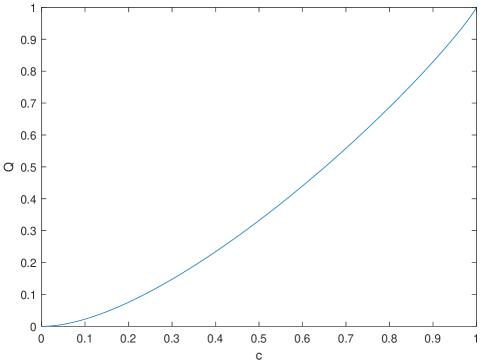
Theorem 3.3.
For the Werner-GHZ state , where , the quantum discord is
(3.27)
Proof.
Obviously, Let , then
(3.28)
It is easy to see that is monotonically increasing with respect to . So .
Fig.1 shows the behavior of the function .
Figure 1. The behavior of the quantum discord for the Werner-GHZ state in Theorem 3.3.
∎
Next, we consider the following general tripartite state
(3.29)
Let and ,
then we can get the quantum discord for some special cases.
Theorem 3.4.
For the general tripartite state in Eq.(3.29), we have the following results:
Case 1: when , we have that
(3.30)
where .
Case 2: when , we have that
(3.31)
where .
Case 3: when , we have that
(3.32)
where .
Case 4: when , we have that
(3.33)
Case 5: when , we have that
(3.34)
Case 6: when , we have that
(3.35)
Proof.
All cases can be shown similarly. Let’s consider case 1: , . Let , then
(3.36)
where .
The derivative of over is equal to
(3.37)
Obviously, when . Then is a strictly increasing function and .
Let ,
, , , .
Imposing , we have . So and , then case 1 is shown.
∎
Example 1. For a state in Eq.(3.1), when .
According to the case 1 of Theorem 3.2, we have . Fig. 2 shows the behavior of the quantum discord .
Figure 2. The behavior of the quantum discord with respect to the parameters in Example 1. In this case, , the quantum discord is only related to variables . Then .
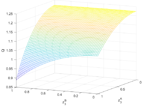
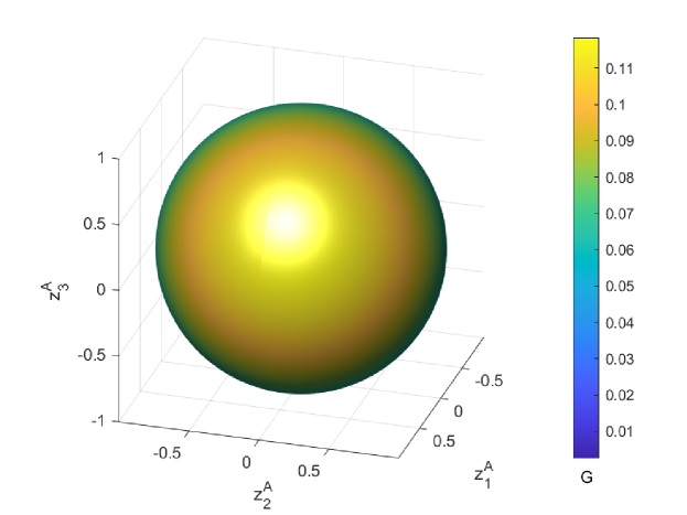
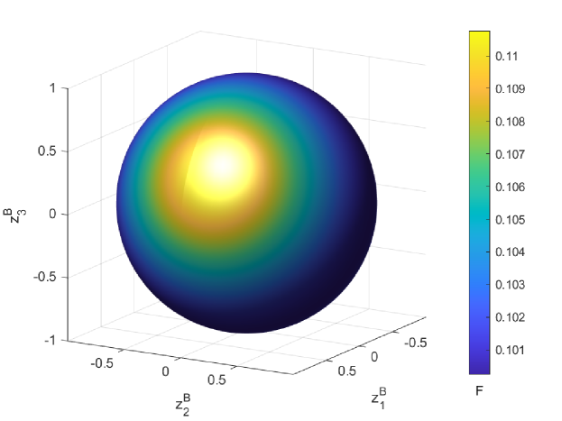
Example 2. For a state of the case 1 in Theorem 3.4, when .
Then the quantum discord is . Fig. 3 and Fig. 4 show the behavior of the function and respectively.
Figure 3. The behavior of with the variables in Example 2, where is on a unit sphere. This is a four-dimensional figure. Among them, the intensity of light is used to indicate the magnitude of the value. The brighter the point, the greater the value of and .Figure 4. The behavior of with the variables in Example 2, where is on a unit sphere. The brighter the point, the greater the value of and .
4. Conclusions
Quantum discord is one of the important correlations in studying quantum systems. It is well-known that the quantum discord is hard to compute explicitly, and only sporadic formulas are known, for instance, the Bell state and the X-state etc. Recently important progresses are made to generalize the notion to multipartite quantum systems [10], and their explicit formulas are expectedly not easy to find. In this work, we have found explicit formulas of the quantum discord for tripartite non X-states with 14 parameters, including some famous states such as the Werner-GHZ state.
Acknowledgments
The research is supported in part by the NSFC
grants 11871325 and 12126351, and Natural Science Foundation of Hubei Province
grant no. 2020CFB538 as well as Simons Foundation
grant no. 523868.
References
[1] Datta, A., Shaji, A., Caves, C. M.: Quantum discord and the power of one qubit, Phys. Rev. Lett., 2008, 100:050502.
[2] Cui, J., Fan, H.: Correlations in the Grover search, J. Phys. A:Math. Theor., 2010, 43(4): 045305.
[3] Ollivier, H., Zurek, W. H.: Quantum discord: a measure of the quantumness of correlations, Phys. Rev. Lett., 2001, 88(1): 017901.
[4] Luo, S.: Quantum discord for two-qubit systems, Phys. Rev. A, 2008, 77(4): 042303.
[5] Rulli, C. C., Sarandy, M. S.: Global quantum discord in multipartite systems, Phys. Rev. A, 2011, 84: 042109.
[6] Okrasa, M., Walczak, Z.: Quantum discord and multipartite correlations, Euro. Phys. Lett., 2011, 96:60003.
[7] Giorgi, G. L., Bellomo, B., Galve, F., et al.: Genuine quantum and classical correlations in multipartite systems,
Phys. Rev. Lett., 2011, 107:190501.
[8] Chakrabarty, I., Agrawal, P., Pati, A. K.: Quantum dissension: Generalizing quantum discord for three-qubit states,
Euro. Phys. J. D, 2011, 65(3):605-612.
[9] Modi, K., Paterek, T., Son, W., et al.: Unified view of quantum and classical correlations, Phys. Rev. Lett., 2010, 104:080501.
[10] Radhakrishnan, C., Laurière, M., Byrnes, T.: Multipartite generalization of quantum discord, Phys. Rev. Lett., 2020, 124: 110401.
[11] Jing, N., Zhang, X., Wang, Y.-K.: Comment on “One-way deficit of two qubit X states”, Quant. Inf. Process, 2015, 14:4511–4521
[12] Streltsov, A. Quantum discord and its role in quantum information theory, In: Quantum
Correlations beyond Entanglement, Springer Briefs in Phys. (New York: Springer), 2015, pp 22-43.
[13] Ye, B., Fei, S.-M.: A note on one-way quantum deficit and quantum discord, Quant. Inf.
Process, 2016, 15:279.
[14] Jing, N., Yu, B.: Quantum discord of X-states as optimization of a one variable function, J. Phys. A:Math. Theor., 2016, 49(38): 385302.
[15] Wilde, M. M.: Quantum information theory, Cambridge University Press, Cambridge, 2017, 2nd. ed.
[16] Vedral, V. The role of relative entropy in quantum information theory, Rev. Mod. Phys., 2002, 74(1): 197.
[17] Groisman, B., Popescu, S., Winter, A.: Quantum, classical, and total amount of correlations in a quantum state, Phys. Rev. A, 2005, 72(3): 032317.
[18] Schumacher, B., Westmoreland, M. D.: Quantum mutual information and the one-time pad, Phys. Rev. A, 2006, 74(4): 042305.