Quantum Disturbance without State Change:
Soundness and Locality of Disturbance Measures
Abstract
It is often supposed that a quantum system is not disturbed without state change. In a recent debate, this assumption is used to claim that the operator-based disturbance measure, a broadly used disturbance measure, has an unphysical property. Here, we show that a quantum system possibly incurs an operationally detectable disturbance without state change to rebut the claim. Moreover, we establish the reliability, formulated as soundness and locality, of the operator-based disturbance measure, which, we show, quantifies the disturbance on an observable that manifests in the time-like correlation even in the case where its probability distribution does not change.
1 Introduction
Heisenberg’s error-disturbance relation (EDR)
| (1) |
for the mean error of a measurement of an observable in any state and the mean disturbance caused on an observable , originally introduced by the -ray microscope thought experiment [1], has been commonly believed as a dynamical aspect of Heisenberg’s uncertainty principle, which is formally represented by a rigorously proven relation
| (2) |
for the indeterminacies, defined as the standard deviations , of arbitrary observables in any state [1, 2, 3]. There have been longstanding research efforts to prove Heisenberg’s EDR [4, 5, 6, 7, 8], while the universal validity has not been reached. Instead, a recent study [9, 10] revealed a universally valid form of EDR
| (3) |
where and are the standard deviations just before the measurement, and made Heisenberg’s EDR testable [10, 11] to observe its violations, confirming the new relation as well [12, 13, 14]. Subsequently, stronger EDRs were derived [15, 16, 17, 18], and confirmed experimentally [19, 20, 21, 22, 23, 24].
In order to define the error and disturbance in Eq. (3), we suppose that the measurement of is described by an interaction from time to between the system in a state and the probe prepared in a fixed state , and that the outcome of the measurement is obtained by the measurement of the meter observable in the probe at time . 111 Note that this general description of a measuring process, also called an indirect measurement model [10], is introduced and proved in Ref. [25] to be equivalent to the most general description using a completely positive instrument, or a so-called quantum instrument, which is a reformulation of the Davies-Lewis instrument [26] with the additional requirement of complete positivity.
In the Heisenberg picture, we shall write , , , for observables in and in , where is the unitary evolution operator for from to . The error and disturbance in Eq. (3) are defined by
| (4) | |||
See Ref. [10] for details. We call and as the operator-based error measure and the operator-based disturbance measure. We shall write and when no confusion may occur.
In the previous work [18], we have investigated the properties of the operator-based error measure (called therein as noise-operator-based quantum root-mean-square error) , and we have introduced its completion , the locally uniform quantum root-mean-square error, and subsequently we have experimentally tested [27] the completeness of and to show how hidden error in manifests in the defining procedure of .
In the present work, we focus on the properties, soundness and locality, of the operator-based disturbance measure , where soundness generally requires a disturbance measure to assign the value 0 to “non-disturbing” measurements, and locality generally requires a disturbance measure to assign the value 0 to “non-disturbing” local measurements.
We say that a measurement is distributionally non-disturbing to an observable in the system state if and have identical probability distributions in the initial state . Korzekwa, Jennings, and Rudolph [28] criticized the use of the operator-based disturbance measure, based on the following requirement for disturbance measures.
Distributional requirement (DR) for disturbance measures. Any disturbance measure should assign the value 0 to distributionally non-disturbing measurements.222 Note that KJR [28] called distributionally non-disturbing measurements as “operationally non-disturbing measurements”; see Eq. (2) in KJR [28].
KJR [28] called the DR “the commonly accepted and operationally motivated requirement that all physically meaningful notions of disturbance should satisfy”. They claimed that the operator-based disturbance measure does not satisfy the DR and has even an ‘unphysical’ property, since it takes a positive value for a measurement that does not change the state at all. Further, they concluded that state-dependent formulations of EDRs are not tenable.
In this paper, we examine the validity of the DR. For this purpose, we consider a more fundamental principle in quantum mechanics, the correspondence principle, stating that if the classical description is available, quantized concepts should be consistent with the classical description. We argue that the DR violates the correspondence principle. We generally show that even if the measurement does not change the state, the disturbance is operationally detectable as long as the operator-based disturbance measure takes a positive value. Thus, the claims made by KJR are groundless. The DR requires that disturbance measures only count the change of the probability distribution in time, but according to the correspondence principle, valid disturbance measures should also count the change of the observable that manifest in the time-like correlation, as the operator-based disturbance measure does.
Moreover, we show that the DR violates another fundamental requirement for no-signaling under local operations, called the locality requirement. Subsequently, we show that disturbance measures satisfying the DR cannot be used to demonstrate the security of quantum cryptography, because they do not properly describe the disturbance caused by the eavesdropper. In contrast, we show that the operator-based disturbance measure satisfies the correspondence principle and the locality requirement. Based on those arguments, we shall conclude that state-dependent formulations of EDRs based on the operator-based disturbance measure reliably represent the originally motivated dynamical aspect of Heisenberg’s uncertainty principle.
2 Correspondence principle
The correspondence principle generally states that quantum theory should be consistent with classical theories in the case where the classical descriptions are also available.333 “The term [the correspondence principle] codifies the idea that a new theory should reproduce under some conditions the results of older well-established theories in those domains where the old theories work [Wikipedia https://en.wikipedia.org/wiki/Correspondence˙principle (August 1, 2022)]”. In fact, it is a common practice to apply classical descriptions to commuting observables through their joint probability distributions. In Ref. [18] we consider the correspondence principle as a requirement for error measures. Here, we extend the consideration to disturbance measures.
It is well-known that any commuting observables have their joint probability distribution in any state. Here, for a given state , the joint probability distribution (JPD) of any two observables is defined as a 2-dimensional probability distribution satisfying
| (5) |
for every (non-commutative) polynomial of and . In general, two observables have their JPD in a state if and only if they commute in in the sense that
| (6) |
where and are the spectral projections of and (Ref. [18], Theorem 1). In this case, the JPD is uniquely determined by
| (7) |
The JPD determines the (classical) root-mean-square deviation between the classical random variables and , the notion originally introduced by Gauss [29], by
| (8) |
We say that a disturbance measure satisfies the correspondence principle (CP) if provided that and have their JPD in the initial state . An important property of the operator-based disturbance measure is that it satisfies the CP, as easily follows from Eq. (5). Similarly, the operator-based error measure also satisfies CP in the sense that provided that and have their JPD in the initial state as shown in Ref. [18].
If and have their JPD , the correlation between and has the classical picture described by , and the classical notion of the root-mean-square deviation is applicable to quantifying the disturbance of . In this case, according to the correspondence principle, any quantum definition of a disturbance measure should be consistent with the classical measure . Thus, we say that a quantum disturbance measure satisfies the correspondence principle if two measures, the quantum and the classical , are consistent, whenever the classical picture is available, as a desirable property of a quantum disturbance measure. In this sense, the correspondence principle determines the value of the disturbance on , when the joint probability distribution of and exists, in an analogous way as the probability distribution of determines its standard deviation appearing in Eq. (3).
3 Disturbing observables without state change
KJR [28] identified as ‘unphysical’ the property of the operator-based disturbance measure that it does not assign the value 0 in a case where the state has not changed at all. In such a case, the probability distribution of every observable has not changed, so that this is a stronger violation of the DR. However, we shall show here that this is not a peculiarity of the operator-based disturbance measure, but a straightforward consequence of the CP.
Consider a qubit measurement. The projective measurement of in the state does not change the initial state . In this case, it was shown [30] that the operator-based disturbance measure indicates that is disturbed by the amount , and this value was actually obtained by a neutron optical experiment [19]. However, according to the DR, every disturbance measure should assign the value 0, and KJR [28] identified the above property of as a very unphysical property. In contrast, we shall show that every disturbance measure satisfying the CP assigns the value .
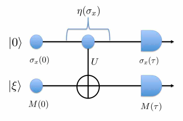
It is well-known that the projective measurement of is carried out by the controlled-NOT operation
| (9) |
for the measured qubit and the probe qubit prepared in the fixed state from to and by the subsequent meter measurement for in (Figure 1) . The Schrödinger time evolution satisfies
| (10) | ||||
| (11) |
For the Heisenberg time evolution is given by
| (12) | ||||
| (13) |
Here, Eq. (13) follows from
It follows that and commute and they have the JPD in the state as
| (14) |
Then we obtain
| (15) |
(cf. Section 9). Thus, if the disturbance measure satisfies the CP, we have
| (16) |
Therefore we conclude . Thus, the non-zero value is not a peculiar property of the operator-based disturbance measure.
It will be instructive to compare the above scenario (1) that the system is prepared in the sate and then a projective measurement of is performed and another scenario (2) that the system is prepared in the sate but no measurement is performed. In both scenarios, the system state is unchanged and the probability distribution of any observable does not change. How can we operationally distinguish the two scenarios. In scenario 1 we have shown that the observable is disturbed. For the time just before the measurement and the time just after the measurement, we obtain and (cf. Eqs. (12) and (13)). Their joint probability distribution satisfies for any (cf. Eq. (15)) that leads to . On the other hand, scenario 2 is easily analyzed, so that we obtain , and their joint probability distribution satisfies that leads to . The joint probability distributions can be experimentally obtained by weak measurements and post-selections as proposed by Lund and Wiseman [11]. Thus, we can operationally distinguish between the above two scenarios.
This conclusion might sound counter-intuitive, as the pure sate has the “maximal information” about the system. However, unchanging the pure state does not imply unchanging the observable, because the “maximal information” about the system does not include the “maximal information” about an observable, analogously with the fact that the “maximal information” about the whole system does not include the “maximal information” about subsystems.
In fact, according to the available classical description, the conditional probability
| (17) |
shows that the value of has been completely randomized, although their marginals have not changed at all as
| (18) |
Thus, the DR neglects the disturbance caused by the randomization by measurement without changing the probability distribution.
4 State-dependent formulation for non-disturbing measurements
We have shown that the DR with the notion of probability non-disturbing measurements contradicts the CP. To reconcile the conflict, we shall characterize non-disturbing measurements from the two fundamental requirements: the CP and the operational accessibility.
Consider the following condition.
(S) and have their JPD in satisfying that if .
From the point of view of the CP, if condition (S) holds, we should conclude that the measurement does not disturb in . Thus, condition (S) is considered as a sufficient condition for a proper definition of non-disturbing measurements.
On the other hand, from the point of view of operational accessibility, it is convenient to consider the weak joint distribution (WJD) of and in defined by
| (19) |
The WJD always exists, though possibly takes negative or complex values, and is operationally accessible by weak measurement and post-selection [31, 32, 33]; see also Ref. [34] for a short survey. Then it is natural to consider the following condition.
(W) The WJD of and in satisfies that if .
If the measurement does not disturb the observable in , any operational tests for witnessing the disturbance should fail. Since measuring WJD is one of such operational tests for which the disturbance is detected if for some [35, 36], condition (W) is considered as a necessary condition for a proper definition of non-disturbing measurements.
Obviously, (W) is logically weaker than or equivalent to (S). However, Theorem 1 (Section 10) shows that both conditions are actually equivalent. In fact, according to the theory of quantum perfect correlations [37, 38], both conditions (S) and (W) equivalently require that and are perfectly correlated in the state [34]. Thus, the above argument justifies the following definition of non-disturbing measurements. We say that the measurement is properly non-disturbing to an observable in if one of the conditions (S) or (W) is satisfied. Since the WJD is operationally accessible, this definition is also operationally accessible.
5 Reliability of the operator-based disturbance measure
To consider the reliability of the operator-based disturbance measure, we examine the following requirements: (i) the CP, (ii) soundness, (iii) operational accessibility, and (iv) completeness.
We have already shown that the operator-based disturbance measure satisfies the CP, i.e., if and have the JPD . We introduce the soundness requirement: Any disturbance measure should assign the value 0 to any properly non-disturbing measurements. It is interesting to see that the CP implies soundness. To show this, suppose that the measurement is properly non-disturbing to in . Then and have the JPD satisfying that if . It follows that and by the CP we have . Accordingly, the operator-based disturbance measure satisfies the soundness requirement. We conclude, therefore, that even if the measurement does not change the state, the disturbance can be operationally detected as long as the operator-based disturbance measure takes a positive value.
It has been known that the operator-based disturbance measure is operationally accessible in the two ways: (i) the tomographic three state method, proposed by Ozawa [10] and experimentally realized by Erhalt et al. [12] and others [14, 19, 23] and (ii) the weak measurement method, proposed by Lund and Wiseman [11] and experimentally realized by Rozema et al. [13] and others [20, 22, 21].
As the converse of soundness, a disturbance measure is said to be complete if assigns the value 0 only to properly non-disturbing measurements. There is an example in which does not satisfy completeness (Ref. [38], p. 750). However, it is known that satisfies completeness if (i) (commutative case) and commute in or if (ii) (dichotomic case) (Ref. [18], Theorem 3).
We have seen that the operator-based disturbance measure satisfies all requirements (i)–(iii), and partially satisfies requirement (iv) above.
Analogously from an argument for the operator-based error measure in Ref. [18], it follows that can be modified to satisfy completeness by defining the operator-based locally uniform disturbance measure as
| (20) |
Then the error measure satisfies requirements (i) – (iv) and also (v) (Dominating property) for any , and (vi) (Conservation property for dichotomic measurements) if . Thus, all the EDRs for also holds for ; see analogous discussions for the operator-based error measure in Ref. [18].
In the following we shall discuss another requirement on locality, which the operator-based disturbance measure satisfies, but contradicts the DR.
6 Locality of disturbance
We have argued that state-dependent formulations of error-disturbance relations are well-founded by the operator-based disturbance measure, which is a sound disturbance measure according to the notion of properly non-disturbing measurement that is supported by the CP and operational accessibility, in contrast to KJR’s claim that the operator-based disturbance measure is not sound under the notion of distributionally non-disturbing measurements, which we have shown to contradict the CP.
Yet, there is a prevailing view that only probability distributions of outcomes of measurements can be operationally compared [39], despite the fact that the new experimental techniques enable us to operationally detect the change of an observable in time: (i) the tomographic three state method [10, 12, 14, 19, 23] and (ii) the weak measurement method [11, 13, 20, 22, 21].
In what follows, we shall show below another drawback of the DR that the notion of probability non-disturbing measurements violates a locality requirement to be posed below.
Consider a composite system in a state . Since any local measurement of does not interact with the system , we naturally take it for granted that any local measurement of non-disturbing to an observable in should be non-disturbing to the observable for any observable in . We call this requirement the locality requirement for a definition of disturbing measurements. We shall show that the definition of distributionally non-disturbing measurements does not satisfy this requirement, whereas the definition of properly non-disturbing measurements does satisfy the requirement as shown in Theorem 2 (Section 11),
For this purpose, we consider a maximally entangled two-qubit system in the Bell state . Since , the outcomes of the joint local measurements of the observables and show a perfect correlation. From Theorem 4 (Section 11), measurements properly non-disturbing to does not change the JPD of and , so that the perfect correlation between and is not disturbed. However, we shall show that a probability non-disturbing measurement breaks the perfect correlation, and this concludes that the definition of probability non-disturbing measurements does not satisfy the locality requirement, according to Theorem 3 (Section 11).
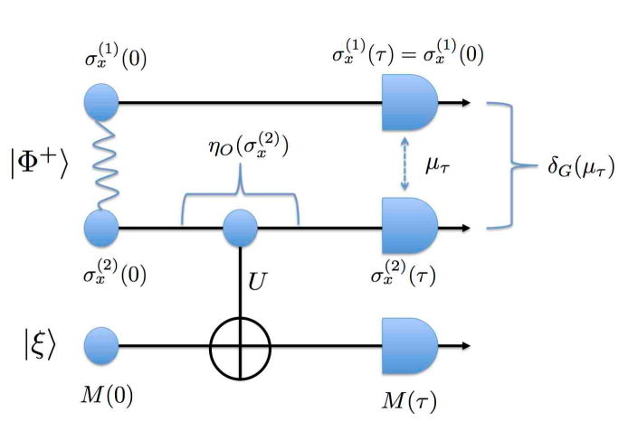
(i) Projective measurement.
Suppose that the observer makes a projective measurement just before the joint local measurements of and (Figure 2 (i)). The measuring interaction is given by
| (21) |
turned on from to between and the probe prepared in with the meter . The time evolutions of relevant observables are given by
| (22) | |||
| (23) | |||
| (24) | |||
Then we shall see that the projective measurement is distributionally non-disturbing to , but it disturbs the perfect correlation between and . To show that, let be the JPD of and for . Then we have
| (25) |
for any (cf. Section 12.1). Since the marginal probability for does not change, the projective measurement is distributionally non-disturbing to . However, the perfect correlation between and at time has been disturbed. The amount of the disturbance of the perfect correlation, i.e., , is measured by the classical root-mean-square deviation , and we have
| (26) |
(cf. Section 12.1). Thus, the projective measurement is distributionally disturbing to for some observable of by Theorem 3 (Section 11). Therefore, we conclude that the definition of distributionally non-disturbing measurements does not satisfy the locality requirement.
Since all observables are mutually commuting, we have their joint probability distribution. The relation holds with probability one by entanglement, and holds by locality of the measurement. Thus, we have
| (27) |
From this and the relation above, we obtain
| (28) |
Thus, we have the conditional probability
| (29) |
showing that is completely randomized by the measuring interaction, whereas the DR neglects this randomization manifest in the joint probability of outcomes of local measurements of and .
(ii) Projective measurement.
For quantitative considerations, suppose that the observer makes a projective measurement just before the joint local measurements of and , where for (Figure 2 (ii)). Then the projective measurement is distributionally non-disturbing to the observable (cf. Section 12.2). However, they disturb the perfect correlation between and . In fact, the JPD of and is given by
and the classical root-mean-square deviation and the disturbance are given by
| (30) |
(cf. Section 12.2). Thus, the joint probability distribution of the outcomes of joint local measurements of and favors the non-zero value , in contrast to the DR requiring .
(iii) Arbitrary local measurements.
Suppose that the observer makes an arbitrary local measurement of from to with the probe prepared in just before the joint local measurements of and (Figure 2 (iii)). Then the JPD and the classical root-mean-square deviation satisfy and . From Theorem 5 (ii) (Section 12), the relation
| (31) |
holds for any local measurement of . Since if and only if is properly non-disturbing to from Theorem 5 (iii) (Section 12), we conclude if and only if is properly non-disturbing to .
Since Eq. (31) holds for an arbitrary local measurement, it has an interesting application to quantum cryptography protocol E91 [40]. Suppose that Alice and Bob share a maximally entangled pair in and that Eve measures for eavesdropping the shared key. Suppose that Alice and Bob share a key encoded in and . To estimate how much information leaks to Eve, cooperative Alice and Bob measure the error probability defined by . Let be Eve’s error for measurement and let be Eve’s disturbance caused on . Then Eq. (31) serves as a bridge between and the disturbance , and the error-disturbance relation further relates with Eve’s error probability for eavesdropping on the key defined by , as follows. Recall that the tight EDR
| (32) |
holds for and (Ref. [17], Eq. (28)). Then this optimizes Eve’s error probability as
| (33) |
Thus, if the entanglement is not disturbed, i.e., , then Alice and Bob conclude to ensure that no information has leaked to Eve. On the other hand, if Eve makes the projective measurement of with , then she has the complete information but this is detected by Alice and Bob as and . However, the DR forces any disturbance measure to assign . How does the DR work to analyze the security of quantum communication?
7 Defense of state-dependent formulations
In order to examine the reliability of the operator-based disturbance measure, KJR [28] introduced the following definition. A state is called a zero-noise zero-disturbance (ZNZD) state with respect to observables and if the projective measurement of in the state , which always satisfies , is distributionally non-disturbing to . Then they proved that for every pair of non-commuting observables and , there exists a ZNZD state such that . Thus, if the disturbance measure satisfies the DR, any relation of the form
| (34) |
where , must be violated. From this, KJR [28] concluded that any state-dependent EDR, based on the expectation value of the commutator as a lower bound, is not tenable, and that state-independent formulations are inevitable.
We have two objections to their claims. First of all, the universally valid relation (3) with leads to the relation
| (35) |
for any projective measurement of in any ZNZD state such that . Thus, the measurement is properly disturbing to by the soundness of , and consequently the disturbance is operationally detectable by the operational accessibility of the definition of properly non-disturbing measurements, so that the assumption by KJR [28] that in any ZNZD state is unfounded.
Secondly, they concluded that state-independent formulations are inevitable for alternative formulations. However, currently proposed state-independent formulations of EDRs [41, 39, 42] do not appear to capture the essence of Heisenberg’s original idea. Recall that Heisenberg derived his EDR by the -ray microscope thought experiment, in which the EDR is derived from the relation between the resolution power and the Compton recoil, reciprocally relating to the wave length of the incident light. Since the wave length is independent of the state of the object, the above formulation might be considered as state-independent. However, the analysis is valid only state-dependently, since the resolution power of the microscope can be defined by the wave length only in the limited situation in which the object is properly placed in the scope of the microscope. Thus, we can adequately define the error of the -ray microscope only state-dependently. In the state-independent formulations, currently one defines the state-independent error as the worst case of the state-dependent error, which must diverge to infinity as the object wave function spreads out of, or moves far apart from, the scope of the microscope. Such state-independent definitions would facilitate to reproduce the form of Heisenberg’s original formulation, but do not keep the physics underlying it. Thus, state-dependent formulations are inevitable to represent Heisenberg’s original idea underlying the uncertainty principle.
8 Discussion
In this paper, we have given a definition of non-disturbing measurement from the point of view of the correspondence principle and operational accessibility. Subsequently, we have established the reliability of the operator-based disturbance measure. We have already discussed the reliability of the operator-based error measure in our previous work [18]. Both accounts ensure that universally valid EDRs [9, 15, 16, 17] reliably represent a dynamical aspect of Heisenberg’s uncertainty principle besides the well-established relation for the indeterminacy in quantum states representing a kinetic aspect of the principle. Thus, the objections to state-dependent formulations of EDRs shown in [39, 28] are unfounded, although those views appear to still prevail in the literature [43, 44]. We conclude that the theory [9, 10, 11, 15, 16, 17, 18] and experiments [12, 13, 19, 14, 21] for state-dependent formulations of EDRs are reliable and that state-dependent formulations are inevitable to represent Heisenberg’s original idea underlying the uncertainty principle.
The new quantitative methods developed in this paper for universally valid EDRs with the well-defined operator-based disturbance measure incorporating with the methods of weak values and weak measurements will provide new quantitative methods to understand the change, transfer, or disturbance of observables in time, which does not manifest in the change of the probability distribution, but which does manifest in the time-like correlation. This quantity will be useful and even inevitable for exploring foundational problems in quantum physics including the long-lasting controversy over the roles of uncertainty principle in which-way measurements for interferometers (Refs. [45, 46, 35, 36, 47] and the references therein). In addition to the foundational problems, it will be expected that universally valid EDRs call for new research interests in exploring various frontiers in physics including fault-tolerant quantum computing [48, 49, 50], quantum metrology [51, 52, 53], and multi-messenger astronomy [54], in which technological limits would be overcome by the fundamental principle independent of particular models. We hope that the methods of operator-based disturbance measures as well as operator-based error measures will be accepted for broad areas of quantum physics.
9 Projective measurement
10 Equivalence for properly non-disturbing measurements
Theorem 1.
Let be a measurement of a system in a state carried out by a measuring interaction with a probe prepared in a fixed state from to . Then for any observable in , the following conditions are equivalent.
(i) Condition (W): The WJD of and in satisfies that if .
(ii) The relation
holds for any .
(iii) Condition (S): and have their JPD in satisfying that if .
Proof.
The assertion was generally proved in Refs. [37, 38] after a lengthy argument. We give a direct proof for the present context.
(i)(ii): Suppose (i) holds. Then the WJD of and in satisfies if . It follows that . Thus,
Consequently,
and
Thus, condition (ii) holds and the implication (i)(ii) follows.
(ii)(iii): Suppose (ii) holds. Then
Consequently,
It follows that and commute in and condition (S) holds. Thus the implication (ii)(iii) follows.
Since the implication (iii)(i) holds obviously, all conditions (i) – (iii) are equivalent. ∎
11 Locality of properly non-disturbing measurements
Theorem 2.
The definition of properly disturbing measurements satisfies the locality requirement.
Proof.
Let be a local measurement of in a composite system in a state . Without any loss of generality that is carried out by a measuring interaction with a probe prepared in a state from time to . Suppose that is properly non-disturbing to an observable in . Let be a polynomial in . From Theorem 1 (ii) (Section 10) we have
Let be an observable in . Let be a polynomial in . Since by the locality of we have
It follows from linearity that
for any polynomial in , and in particular we have
Thus, does not disturb for any in by Theorem 1 (ii) (Section 10). Therefore, the definition of properly disturbing measurements satisfies the locality requirement. ∎
Theorem 3.
Let be a composite system in a state . Let be an observable in . Any local measurement of distributionally non-disturbing to for any in does not change the JPD of observable and for any observable in .
Proof.
Let be an observable in and . By assumption, does not change the probability distribution of , so that all moments of are unchanged as
for all . By linearity, we have
for any polynomial in . It follows that
and hence does not change the JPD of and for any observable in . ∎
Theorem 4.
Let be a composite system in a state . Any local measurement of properly non-disturbing to in does not change the JPD of observable and for any observable in .
12 Operator-based disturbance measure and disturbance of entanglement
Theorem 5.
Let be a composite system in a state . Let be a local measurement of the system carried out by a measuring interaction with a probe prepared in a fixed state from to . Let be the JPD of an observable in and an observable in for . Let be the operator-based disturbance of for . Let be the classical root-mean-square deviation determined by . Then we have the following.
(i) The relation
holds.
(ii) If then .
(iii) If and then is properly non-disturbing to if and only
Proof.
(i) We have the relations
and hence assertion (i) follows from repeated uses of the triangular inequality.
(ii) Follows by substituting in (i).
(iii) Follows from (ii) and the completeness of for dichotomic observables. ∎
12.1 Projective measurement
Consider the projective measurement of in carried out by the measuring interaction
turned on from to between and the probe prepared in with the meter observable . Consider the Heisenberg operators and for . From Eq. (13) we have
Let be the JPD of and in the state . We shall show
(i) ,
(ii) ,
(iii) .
We have
and (i) follows.
We have
Consequently,
Similarly,
Thus, we have
for any , and (ii) follows. Thus, Eq. (25) is obtained.
12.2 Projective measurement
Suppose that the observer makes a measurement of in , carried out by the measuring interaction
turned on from to and by the subsequent measurement of the meter observable of prepared in . This realizes the projective measurement of as
for , where and . Consider the Heisenberg operators and for . We have
Let for be the JPD of and in the state , i.e.,
Then we have
For we have
We used the parallelogram law twice in the third last and the penultimate equalities. It follows that
Thus, with , the projective measurement of is distributionally non-disturbing to .
Let be the classical root-mean-square deviation for . We have . By Theorem 5 (ii) we have Then from (Ref. [12], Eq. (6)) we have
Thus, we obtain Eq. (30), i.e.,
In what follows we will determine without tedious calculations on relevant projections. We have
Since and is distributionally non-disturbing to , we have
Since,
we obtain
It follows that
Therefore, we have derived Eq. (LABEL:eq:entanglement-3).
References
- [1] Heisenberg, W. Über den anschaulichen Inhalt der quantentheoretischen Kinematik und Mechanik. Z. Phys. 43, 172–198 (1927).
- [2] Kennard, E. H. Zur Quantenmechanik einfacher Bewegungstypen. Z. Phys. 44, 326–352 (1927).
- [3] Robertson, H. P. The uncertainty principle. Phys. Rev. 34, 163–164 (1929).
- [4] Arthurs, E. and Kelly, Jr., J. L. On the simultaneous measurement of a pair of conjugate observables. Bell. Syst. Tech. J. 44, 725–729 (1965).
- [5] Yamamoto, Y. and Haus, H. A. Preparation, measurement and information capacity of optical quantum states. Rev. Mod. Phys. 58, 1001–1020 (1986).
- [6] Arthurs, E. and Goodman, M. S. Quantum correlations: A generalized Heisenberg uncertainty relation. Phys. Rev. Lett. 60, 2447–2449 (1988).
- [7] Ishikawa, S. Uncertainty relations in simultaneous measurements for arbitrary observables. Rep. Math. Phys. 29, 257–273 (1991).
- [8] Ozawa, M. Quantum limits of measurements and uncertainty principle. In Bendjaballah, C., Hirota, O. and Reynaud, S. (eds.) Quantum Aspects of Optical Communications, 1–17 (Springer, Berlin, 1991).
- [9] Ozawa, M. Universally valid reformulation of the Heisenberg uncertainty principle on noise and disturbance in measurement. Phys. Rev. A 67, 042105 (2003).
- [10] Ozawa, M. Uncertainty relations for noise and disturbance in generalized quantum measurements. Ann. Phys. (N.Y.) 311, 350–416 (2004).
- [11] Lund, A. P. and Wiseman, H. M. Measuring measurement-disturbance relationships with weak values. New J. Phys. 12, 093011 (2010).
- [12] Erhart, J. et al. Experimental demonstration of a universally valid error-disturbance uncertainty relation in spin measurements. Nat. Phys. 8, 185–189 (2012).
- [13] Rozema, L. A. et al. Violation of Heisenberg’s measurement-disturbance relationship by weak measurements. Phys. Rev. Lett. 109, 100404 (2012).
- [14] Sulyok, G. et al. Violation of Heisenberg’s error-disturbance uncertainty relation in neutron spin measurements. Phys. Rev. A 88, 022110 (2013).
- [15] Branciard, C. Error-tradeoff and error-disturbance relations for incompatible quantum measurements. Proc. Natl. Acad. Sci. USA 110, 6742–6747 (2013).
- [16] Branciard, C. Deriving tight error-trade-off relations for approximate joint measurements of incompatible quantum observables. Phys. Rev. A 89, 022124 (2014).
- [17] Ozawa, M. Error-disturbance relations in mixed states (2014). URL https://arxiv.org/abs/1404.3388.
- [18] Ozawa, M. Soundness and completeness of quantum root-mean-square errors. npj Quantum Inf. 5, 1 (2019).
- [19] Baek, S.-Y., Kaneda, F., Ozawa, M. and Edamatsu, K. Experimental violation and reformulation of the Heisenberg error-disturbance uncertainty relation. Sci. Rep. 3, 2221 (2013).
- [20] Weston, M. M., Hall, M. J. W., Palsson, M. S., Wiseman, H. M. and Pryde, G. J. Experimental test of universal complementarity relations. Phys. Rev. Lett. 110, 220402 (2013).
- [21] Kaneda, F., Baek, S.-Y., Ozawa, M. and Edamatsu, K. Experimental test of error-disturbance uncertainty relations by weak measurement. Phys. Rev. Lett. 112, 020402 (2014).
- [22] Ringbauer, M. et al. Experimental joint quantum measurements with minimum uncertainty. Phys. Rev. Lett. 112, 020401 (2014).
- [23] Demirel, B., Sponar, S., Sulyok, G., Ozawa, M. and Hasegawa, Y. Experimental test of residual error-disturbance uncertainty relations for mixed spin- states. Phys. Rev. Lett. 117, 140402 (2016).
- [24] Liu, Y. et al. Experimental test of error-tradeoff uncertainty relation using a continuous-variable entangled state. npj Quantum Inf. 5, 68 (2019).
- [25] Ozawa, M. Quantum measuring processes of continuous observables. J. Math. Phys. 25, 79–87 (1984).
- [26] Davies, E. B. and Lewis, J. T. An operational approach to quantum probability. Commun. Math. Phys. 17, 239–260 (1970).
- [27] Sponar, S., Danner, A., Ozawa, M. and Hasegawa, Y. Neutron optical test of completeness of quantum root-mean-square errors. npj Quantum Inf. 7, 106 (2021).
- [28] Korzekwa, K., Jennings, D. and Rudolph, T. Operational constraints on state-dependent formulations of quantum error-disturbance trade-off relations. Phys. Rev. A 89, 052108 (2014).
- [29] Gauss, C. F. Theoria Combinationis Observationum Erroribus Miinimis Obnoxiae, Pars Prior, Pars Posterior, Supplementum (Societati Regiae Scientiarum Exhibita, Göttingen, 1821).
- [30] Ozawa, M. Universal uncertainty principle in measurement operator formalism. J. Opt. B: Quantum Semiclass. Opt. 7, S672–S681 (2005).
- [31] Aharonov, Y., Albert, D. Z. and Vaidman, L. How the result of a measurement of a component of the spin of a spin-1/2 particle can turn out to be 100. Phys. Rev. Lett. 60, 1351–1354 (1988).
- [32] Steinberg, A. M. Conditional probabilities in quantum theory and the tunneling-time controversy. Phys. Rev. A 52, 32–42 (1995).
- [33] Jozsa, R. Complex weak values in quantum measurement. Phys. Rev. A 76, 044103 (2007).
- [34] Ozawa, M. Universal uncertainty principle, simultaneous measurability, and weak values. AIP Conf. Proc. 1363, 53–62 (2011).
- [35] Garretson, J. L., Wiseman, H. M., Pope, D. T. and Pegg, D. T. The uncertainty relation in ‘which-way’ experiments: how to observe directly the momentum transfer using weak values. J. Opt. B: Quantum Semiclass. Opt. 6, S506–S517 (2004).
- [36] Mir, R. et al. A double-slit ‘which-way’ experiment on the complementarity-uncertainty debate. New J. Phys. 9, 287 (2007).
- [37] Ozawa, M. Perfect correlations between noncommuting observables. Phys. Lett. A 335, 11–19 (2005).
- [38] Ozawa, M. Quantum perfect correlations. Ann. Phys. (N.Y.) 321, 744–769 (2006).
- [39] Busch, P., Lahti, P. and Werner, R. F. Colloquium: Quantum root-mean-square error and measurement uncertainty relations. Rev. Mod. Phys. 86, 1261–1281 (2014).
- [40] Ekert, A. K. Quantum cryptography based on Bell’s theorem. Phys. Rev. Lett. 67, 661–663 (1991).
- [41] Appleby, D. M. The error principle. Int. J. Theor. Phys. 37, 2557–2572 (1998).
- [42] Appleby, D. M. Quantum errors and disturbances: Response to Busch, Lahti and Werner. Entropy 18, 174 (2016).
- [43] Renes, J. M., Scholz, V. B. and Huber, S. Uncertainty relations: An operational approach to the error-disturbance tradeoff. Quantum 1, 20 (2017).
- [44] Mao, Y.-L. et al. Error-disturbance trade-off in sequential quantum measurements. Phys. Rev. Lett. 122, 090404 (2019).
- [45] Scully, M. O., Englert, B.-G. and Walther, H. Quantum optical tests of complementarity. Nature 351, 111–116 (1991).
- [46] Storey, P., Tan, S., Collett, M. and Walls, D. Path detection and the uncertainty principle. Nature 367, 626–628 (1994).
- [47] Xiao, Y. et al. Observing momentum disturbance in double-slit “which-way” measurements. Sci. Adv. 5, eaav9547 (2019).
- [48] Nielsen, M. A. and Chuang, I. L. Quantum Computation and Quantum Information (Cambridge UP, Cambridge, 2000).
- [49] Ozawa, M. Conservative quantum computing. Phys. Rev. Lett. 89, 057902 (2002).
- [50] Takagi, R. and Tajima, H. Universal limitations on implementing resourceful unitary evolutions. Phys. Rev. A 101, 022315 (2020).
- [51] Ozawa, M. Measurement breaking the standard quantum limit for free-mass position. Phys. Rev. Lett. 60, 385–388 (1988).
- [52] Giovannetti, V., Lloyd, S. and Maccone, L. Quantum-enhanced measurements: Beating the standard quantum limit. Science 306, 1330–1336 (2004).
- [53] Aspelmeyer, M., Kippenberg, T. J. and Marquardt, F. Cavity optomechanics. Rev. Mod. Phys. 86, 1391–1452 (2014).
- [54] Bartos, I. and Kowalski, M. Multimessenger Astronomy. (IOP Publishing, 2017). URL http://dx.doi.org/10.1088/978-0-7503-1369-8.